HAL Id: hal-00785252
https://hal.archives-ouvertes.fr/hal-00785252
Submitted on 12 Feb 2013HAL is a multi-disciplinary open access archive for the deposit and dissemination of sci-entific research documents, whether they are pub-lished or not. The documents may come from teaching and research institutions in France or abroad, or from public or private research centers.
L’archive ouverte pluridisciplinaire HAL, est destinée au dépôt et à la diffusion de documents scientifiques de niveau recherche, publiés ou non, émanant des établissements d’enseignement et de recherche français ou étrangers, des laboratoires publics ou privés.
Hydrological model parameter instability: A source of
additional uncertainty in estimating the hydrological
impacts of climate change?
Pierre Brigode, Ludovic Oudin, Charles Perrin
To cite this version:
Pierre Brigode, Ludovic Oudin, Charles Perrin. Hydrological model parameter instability: A source of additional uncertainty in estimating the hydrological impacts of climate change?. Journal of Hy-drology, Elsevier, 2013, 476, pp.410 - 425. �10.1016/j.jhydrol.2012.11.012�. �hal-00785252�
Hydrological model parameter instability: A source of additional
1
uncertainty in estimating the hydrological impacts of climate
2
change?
3 4
Pierre Brigode1, Ludovic Oudin1, Charles Perrin2 5
1
UPMC Univ. Paris 06, UMR 7619 Sisyphe, Case 105, 4 Place Jussieu, F-75005 Paris, 6
France 7
2
Hydrosystems Research Unit (HBAN), Irstea, 1, rue Pierre-Gilles de Gennes, CS 8
10030, 92761 Antony Cedex, France 9
10
Corresponding author. Email: [email protected] 11
12
1 INTRODUCTION ... 3 13
1.1 Hydrological projections under climate change and their associated uncertainties ... 3
14
1.2 Can model parameter instability be a major source of uncertainty? ... 5
15
1.3 Scope of the paper ... 7
16
2 DATA AND MODELS... 8 17 2.1 Catchment set ... 8 18 2.2 Hydro-meteorological data ... 9 19 2.3 Rainfall-runoff models ... 10 20 2.4 Model parameterisation ... 10 21
3 METHODOLOGY FOR INVESTIGATING PARAMETER UNCERTAINTY IN A CHANGING CLIMATE 22
11
23
3.1 General methodology ... 11
24
3.2 Step 1: Identification of climatically contrasted sub-periods ... 12
25
3.3 Step 2: Model calibrations on the specific periods ... 13
26
3.4 Step 3: Model simulations with different parameter sets ... 14
27
4 RESULTS ... 15 28
4.1 Calibration performance results ... 15
29
4.2 Sensitivity to the climate characteristics of the calibration period ... 17
30
4.3 Sensitivity to the use of a posterior ensemble of parameter sets ... 22
31
5 DISCUSSION AND CONCLUSION ... 26 32 6 ACKNOWLEDGMENTS ... 30 33 7 REFERENCES ... 31 34 8 FIGURES ... 35 35 36 37
Abstract
38
This paper investigates the uncertainty of hydrological predictions due to rainfall-runoff 39
model parameters in the context of climate change impact studies. Two sources of 40
uncertainty were considered: (i) the dependence of the optimal parameter set on the 41
climate characteristics of the calibration period and (ii) the use of several posterior 42
parameter sets over a given calibration period. The first source of uncertainty often refers 43
to the lack of model robustness, while the second one refers to parameter uncertainty 44
estimation based on Bayesian inference. Two rainfall-runoff models were tested on 89 45
catchments in northern and central France. The two sources of uncertainty were assessed 46
in the past observed period and in future climate conditions. The results show that, given 47
the evaluation approach followed here, the lack of robustness was the major source of 48
variability in streamflow projections in future climate conditions for the two models 49
tested. The hydrological projections generated by an ensemble of posterior parameter sets 50
are close to those associated with the optimal set. Therefore, it seems that greater effort 51
should be invested in improving the robustness of models for climate change impact 52
studies, especially by developing more suitable model structures and proposing 53
calibration procedures that increase their robustness. 54
55
Keywords: Climate change, rainfall-runoff modelling, hydrological model calibration,
56
uncertainty, robustness. 57
1 INTRODUCTION
59
1.1 Hydrological projections under climate change and their associated uncertainties
60
The impacts of climate change on catchment behaviour have been extensively investigated 61
over the last few decades (see e.g. for Europe Arnell, 1999a, Arnell, 1999b; for Australia 62
Vaze et al., 2011 and Vaze and Teng, 2011). Quantitatively assessing the uncertainties 63
associated with hydrological projections is a difficult task, even if qualitatively it is now 64
recognised that these uncertainties are considerable. They stem from the methods used to 65
generate climate projections as well as from hydrological modelling. Moreover, the relative 66
importance of the various uncertainty sources is not easy to assess. Wilby and Harris (2006) 67
proposed a framework to assess the relative weights of the sources of uncertainty in future 68
low flows for the River Thames. They consider that uncertainty sources should be ranked in 69
decreasing order as follows: Global Circulation Models (GCMs) > (empirical) downscaling 70
method > hydrological model structure > hydrological model parameters > emission scenario. 71
However, this conclusion was obtained using only two rainfall-runoff models applied to a 72
single catchment. Wilby (2005) noted that depending on the rainfall-runoff model used (and 73
possibly the catchment studied), the uncertainties associated with hydrological modelling may 74
predominate. More recently, Chen et al. (2011) showed on a Canadian catchment that the 75
choices of GCMs and downscaling techniques are the greatest uncertainty sources in 76
hydrological projection estimations, followed by emission scenarios and hydrological model 77
structures, and last hydrological model parameter estimation. On several southeastern 78
Australian catchments, Teng et al. (2012) also showed that uncertainties stemming from 79
fifteen GCM outputs are much greater than the uncertainties stemming from five hydrological 80
models. Focusing on future hydrological trends in the UK, Arnell (2011) showed that 81
“uncertainty in response between climate model patterns is considerably greater than the 82
range due to uncertainty in hydrological model parameterization.” These results show that the 83
uncertainties generated by the hydrological modelling step, though generally lower than that 84
generated by the climate modelling step, can be significant in some cases and should not be 85
ignored in climate change impact studies. 86
The common sources of uncertainty in hydrological modelling in stationary conditions (in 87
terms of climate conditions and/or physical characteristics) include errors in model structure, 88
problems in the calibration procedure, and errors in the data used for calibration. In non-89
stationary conditions, as in climate change studies, additional uncertainties may come from 90
parameter instability due to the possible changes in the physical catchment characteristics and 91
in the dominant processes. In both cases, model structure errors and the identification of 92
model parameters can generally be considered as the two main sources of uncertainty in the 93
hydrological modelling step. Several methods exist for studying uncertainties due to model 94
structure (see e.g. Refsgaard et al., 2006). In climate change impact studies, the errors 95
stemming from the model structure are usually assessed using several rainfall-runoff models 96
and quantifying the range of their outputs (Booij, 2005; Wilby, 2005; Wilby and Harris, 2006; 97
Jiang et al., 2007). The problem of parameter identification has been widely investigated and 98
many methods to quantify the associated uncertainty have been proposed (see e.g. Matott et 99
al., 2009, for a review). In a recent study, Bastola et al. (2011) attempted to quantify these two 100
hydrological uncertainty sources (model structure and parameter sets) in a climate change 101
context using a multi-model approach combining multiple emission scenarios and GCMs, 102
four conceptual rainfall-runoff models and two parameter uncertainty evaluation methods 103
(Generalized Likelihood Uncertainty Estimation and Bayesian Model Averaging). The 104
authors concluded that “the role of hydrological model uncertainty is remarkably high and 105
should therefore be routinely considered in impact studies.” Note that the type of hydrological 106
model used (physically-based or conceptual, lumped or distributed, etc.) may also be 107
considered as an uncertain choice, in both stationary and non-stationary conditions. It is often 108
considered that the physical basis of process descriptions is indispensable to maintain the 109
predictive power of hydrological models in a changing climate (see e.g. Ludwig et al., 2009). 110
A few studies have covered this issue by considering both conceptual and physically-based 111
models (see e.g. Poulin et al., 2011). The RExHySS project (Ducharne et al., 2009; Ducharne 112
et al., 2011) addressed this issue on the Seine River basin (France) by considering seven 113
hydrological models, including distributed (predominantly) physically-based models, semi-114
distributed physically-based models and lumped conceptual models. Interestingly, the results 115
showed that the conceptualisation of the models was not the main source of variability in 116
hydrological projections among the model simulations since large differences were found 117
between models with similar conceptualisations. 118
1.2 Can model parameter instability be a major source of uncertainty?
119
Other studies have investigated the dependence of the model parameters on the characteristics 120
of the record period used for calibration. In climate change impact studies, the record period 121
used to calibrate the model differs from the projected period. Since rainfall-runoff model 122
parameters must be calibrated using the available data sets, they will partially account for the 123
errors contained in these data (see e.g. Yapo et al., 1996; Oudin et al., 2006a) and/or their 124
specific climate characteristics (see e.g. Gan and Burges, 1990). This is a well-known issue 125
for conceptual rainfall-runoff models but physically-based models are also affected by this 126
problem (see e.g. Rosero et al., 2010). Model parameters are the integrators of the data‟s 127
information content. Different time periods used for calibration may provide quite different 128
optimum parameter sets, depending on whether the period is dry or wet, for example, thus 129
providing an estimation of parameter uncertainty with respect to their lack of robustness. Here 130
Beven (1993) states that “it is easy to show that if the same model is „optimised‟ on two 131
different periods of record, two different optimum parameter sets will be produced. Extension 132
to multiple calibration periods, if the data were available, would yield multiple optimum 133
parameter sets. The resulting parameter distributions would reflect the uncertainty in the 134
parameter estimates and the interaction between the individual parameters.” As stressed by 135
Gan and Burges (1990), this obviously “should be heeded by modelers who use calibrated 136
conceptual models to explore hydrologic consequences of climate change.” As a consequence, 137
and without clear guidelines on how the model should be calibrated for climate change impact 138
studies, most hydrologists calibrate their models with all the available data (e.g. Vaze and 139
Teng, 2011) or with the longest observed period they consider representative of the current 140
hydro-climatology conditions (e.g. Poulin et al., 2011), generally considering a priori that “the 141
longer the calibration period, the more robust the parameter set.” 142
One way to evaluate the capacity of models to represent the hydrological behaviour of a 143
catchment in a changing climate is to apply the differential split-sample test, introduced by 144
Klemeš (1986). In this testing scheme, two contrasted periods are identified in the available 145
record and the split-sample test is performed using these two periods. If the model is intended 146
to simulate streamflow under wetter climate conditions, then it should be calibrated on a dry 147
period selected in the available record and validated on a wet period. Conversely, if it is 148
intended to simulate flows under drier climatic conditions, the reverse should be done. The 149
model should demonstrate its ability to perform well in these contrasted conditions. Despite 150
the simplicity of the test, relatively few authors have followed the differential split-sample test 151
in the past (see e.g. Jakeman et al., 1993; Refsgaard and Knudsen, 1996; Donnelly-152
Makowecki and Moore, 1999; Seibert, 2003; Wilby, 2005). More recently, Merz et al. (2011) 153
applied the test to a large set of 273 catchments in Austria and found that the parameters of 154
the hydrological model controlling snow and soil moisture processes were significantly 155
related to the climatic conditions of the calibration period. Consequently, the performance of 156
the model was particularly affected if the calibration and the validation periods differed 157
substantially. Vaze et al. (2010) also applied the differential split-sample test to 61 catchments 158
in southeast Australia with four conceptual hydrological models. They found that the 159
performance of these models was relatively dependent on the climatic conditions of the 160
calibration period. On 216 southeastern Australian catchments, Coron et al. (2012) 161
highlighted the same lack of robustness of three hydrological models tested in climatic 162
conditions different from those used for parameter calibration. Vaze et al. (2010) therefore 163
suggest that it would be wiser to calibrate model parameters on a portion of the record with 164
conditions similar to those of the future period to simulate. This idea was also put forward by 165
de Vos et al. (2010), who proposed dynamically re-calibrating model parameters for each 166
temporal cluster by finding analogous periods in the historical record. Following similar 167
motivations, Luo et al. (2011) showed that more consistent model predictions on specific 168
hydrological years are obtained if a selection of calibration periods is performed, and Singh et 169
al. (2011) used adjusted parameter values depending on the aridity of the catchment 170
considered for improving model prediction. These methodologies could be applied for 171
simulating future hydrological conditions, but unfortunately, as stated by Prudhomme and 172
Davies (2009), long records that include climatic conditions similar to what could be expected 173
in the future are lacking. This makes it difficult to identify a set of parameters specific to such 174
future conditions. Note that in some regions, climate changes have occurred in the past and it 175
is therefore possible to objectively assess the potential of hydrological models to cope with 176
changing climate. This is the case for Central and Western Africa, affected by a marked 177
reduction in rainfall and runoff from the year 1970 onwards. Using different models on 178
different catchments in this region, Niel et al. (2003) and Le Lay et al. (2007) showed no 179
evidence that non-stationarity in climate would incur model parameter instability. 180
1.3 Scope of the paper
181
This paper intends to investigate the uncertainty of hydrological predictions for the future 182
climate. To this aim, we followed Klemeš‟s differential split-sample test and assessed the 183
corresponding variability of the simulated hydrological impacts of projected climate when 184
considering alternatively (i) the dependence of the optimal parameter set on the calibration 185
period characteristics and (ii) an ensemble of posterior parameter sets obtained on a given 186
calibration period. Each source of uncertainty was already studied in the context of changing 187
climate, but their relative importance has not been assessed so far. Besides, most studies 188
focusing on the parameter‟s dependency on climate conditions did not assess the 189
consequences of choosing various calibration strategies on future hydrological projections. 190
Here we will attempt to assess the long-term effects of these two sources of uncertainty in 191
future conditions. 192
193
2 DATA AND MODELS
194
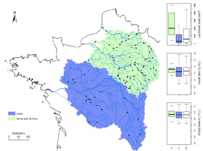
2.1 Catchment set
195
A set of 89 catchments located in northern and central France was used, namely the Somme 196
River at Abbeville, 22 sub-catchments of the Loire River basin and 66 sub-catchments of the 197
Seine River basin (see Figure 1). Catchment area ranges from 32 to 109,930 km², runoff yield 198
ranges from 0.11 to 0.69 and the aridity index (here defined as the ratio of mean annual 199
Penman (1948) potential evapotranspiration to mean annual rainfall) ranges from 0.64 to 1.39. 200
Compared to the Seine basin sub-catchments, the sub-catchments of the Loire River basin add 201
diversity in terms of physiographic characteristics (with generally larger areas, higher 202
elevations, and a different geological context), and hydro-climatic characteristics (with 203
generally higher runoff yields). None of the catchments studied is strongly influenced by 204
upstream dams. 205
FIGURE 1: Location and distribution of various characteristics of the 89 catchments used.
207
The boxplots show the 0.10, 0.25, 0.50, 0.75 and 0.90 percentiles (67 is the number of
208
catchments in the Seine and Somme basins, 22 in the Loire basin).
209
210
2.2 Hydro-meteorological data
211
The hydrological models tested here require only daily time series of potential 212
evapotranspiration (PE) and rainfall (P) as input data. We used climate data from the 213
SAFRAN meteorological reanalysis (Quintana-Segui et al., 2008; Vidal et al., 2010), which 214
provides daily series of Penman PE and P from 1970 to 2007 at a mesoscale (on an 8 × 8 km 215
grid). These data were aggregated for each catchment in order to estimate mean areal inputs. 216
Besides daily streamflow (Q), time series were used to calibrate the models and assess their 217
performance. 218
Since it is not within the scope of this paper to discuss the uncertainties related to climate 219
projections, the outputs of a single general circulation model (GFDL CM2.1) driven by the 220
A1B emissions scenario (IPCC, 2007) were chosen as climate projections. These outputs were 221
regionalised using a statistical downscaling method based on weather types (Boé et al., 2006), 222
producing a database at the same spatial resolution as the SAFRAN database (8 × 8 km). 223
Three time slices with continuous daily series of PE and P were used in this study: 224
1980–2000, referred to as "present time" and noted PT hereafter; 225
2045–2065, referred to as "mid-century" and noted MC hereafter; 226
2080–2100, referred to as "end-of-century" and noted EC hereafter. 227
This scenario was tested on the Seine and the Somme basins within the RExHySS project 228
(Ducharne et al., 2009, Ducharne et al., 2011) and on the Loire River basin within the ICC-229
Hydroqual project (Moatar et al., 2010). For the Seine and the Somme basins, the downscaled 230
projection simulates an increase in mean annual air temperature of 1.8°C by MC and 3.1°C by 231
EC, a decrease in mean annual precipitation of 5% by MC and 10% by EC (with an increase 232
of winter precipitation and a decrease of summer precipitation) and an increase in potential 233
evapotranspiration of 16% by MC and 26% by EC. These predictions are close to the mean 234
trends estimated with up to 14 climate projections used in the RExHySS and ICC-Hydroqual 235
projects, making the scenario used in this study an in-between scenario. 236
2.3 Rainfall-runoff models
237
Two daily continuous lumped rainfall-runoff models were used to avoid providing model-238
specific conclusions: 239
The GR4J rainfall-runoff model, an efficient and parsimonious (four free parameters) 240
model described in detail by Perrin et al. (2003); 241
The TOPMO model (six free parameters), inspired by TOPMODEL (Beven and 242
Kirkby, 1979; Michel et al., 2003), already tested on large data sets. This lumped 243
model is quite different from GR4J but has comparable performance (see e.g. Oudin et 244
al., 2006b). Here the distribution of the topographic index is parameterised and 245
optimised, and not calculated from a digital elevation model. This was found to have 246
only a limited impact on model efficiency, as shown by Franchini et al. (1996) and this 247
eases the application of the model when it is tested on a large set of catchments. 248
Note that we did not explicitly investigate the uncertainties stemming from hydrological 249
model structures. This was analysed e.g. by Seiller et al. (2012) using a multi-model approach 250
in a climate change perspective. 251
2.4 Model parameterisation
252
The optimisation algorithm used to calibrate parameter values is the Differential Evolution 253
Adaptive Metropolis (DREAM) algorithm (Vrugt et al., 2009). DREAM optimises model 254
parameters on a given period and additionally infers the posterior probability distribution of 255
model parameter values through Markov Chain Monte Carlo (MCMC) sampling. 256
As an objective function, we used the formal Generalized Likelihood function described by 257
Schoups and Vrugt (2010), which considers correlated, heteroscedastic, and non-Gaussian 258
errors (noted GL hereafter). The results in validation are analysed with the Nash and Sutcliffe 259
(1970) efficiency criterion, which is still widely used in modelling studies. It was computed 260
on root square transformed flows (noted NSEsq hereafter), which makes it possible to assess 261
model efficiency for both high and low flows (Oudin et al. 2006b). 262
263
3 METHODOLOGY FOR INVESTIGATING PARAMETER UNCERTAINTY IN A CHANGING
264
CLIMATE
265
3.1 General methodology
266
The building blocks of the method originate from the differential split-sample test 267
recommended by Klemeš (1986) and the methodology followed by Wilby (2005). The 268
parameter uncertainty associated with the changing climate is characterised by the variability 269
of the parameters across calibration sub-periods with varying hydroclimatic characteristics. 270
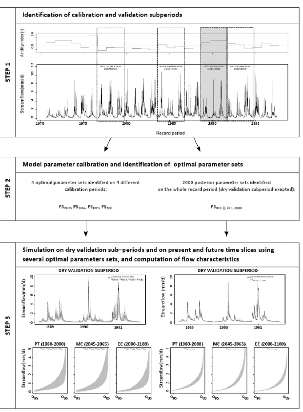
The methodology is carried out in three steps (see Figure 2): 271
Step 1: identification of test periods. 272
Step 2: model parameter calibration and identification of posterior parameter sets. 273
Step 3: model validation and simulation, and parameter uncertainty quantification. 274
These three steps are further detailed hereafter. 275
276
FIGURE 2: Illustration of the three-step methodology used for investigating parameter
277
uncertainty in a changing climate.
279
Note that a similar methodology was used in the RheinBlick project (Görgen et al., 2010) for 280
quantifying uncertainties due to the parameters of hydrological models in a climate change 281
perspective on the Rhine basin. 282
3.2 Step 1: Identification of climatically contrasted sub-periods
283
For each catchment, four climatically contrasted 3-year sub-periods were identified in the 284
available record: a wet period, two dry ones and an intermediate one. The driest sub-285
period will be used as the validation period (hereafter noted dry validation sub-periods) and 286
the three others will be used as calibration sub-periods. This choice was made because the 287
selected climate projection indicates that future conditions will be drier and warmer on the 288
test basins. The aridity index (here defined as the ratio of mean Penman potential 289
evapotranspiration to mean precipitation) was used to characterise the climatic specificity of 290
each sub-period: the wet sub-period corresponds to the three contiguous hydrological years 291
with the lowest aridity index (here a hydrological year starts on September 1 and ends on 292
August 31). The choice of this index is rather arbitrary and may influence the results obtained 293
hereafter. However, since it is solely based on climate characteristics, this makes it possible to 294
assess the climatic specificity of the chosen sub-periods compared to the projected future 295
climate. Obviously, it was not possible to use a criterion based on observed streamflows, as 296
done by Seibert (2003) on observed data, since future flow observations by definition do not 297
exist. 298
The choice of the length of the record sub-period to consider is not straightforward since it is 299
based on a trade-off between two opposite expectations: (i) the longer the sub-periods, the 300
more robust the set of parameters should be and (ii) the shorter the sub-periods, the more 301
climatically contrasted sub-periods can be found in the record period. A review of the 302
literature (see e.g. the review proposed by Perrin et al. (2007)) shows that there is no clear 303
consensus on the minimum length of calibration period for rainfall-runoff models, which is 304
probably attributable to the specificity of the catchments and models used in those studies. 305
Specifically for the two parsimonious models used in this paper, Anctil et al. (2004) obtained 306
good GR4J performance with 3- to 5-year calibration periods and Perrin et al. (2007) showed 307
that the calibration of the GR4J and TOPMO models with the equivalent of only 1 year of 308
data can provide acceptable performance. Thus, it seems that 3-year periods can yield 309
acceptable parameter sets. Those relatively short sub-periods allow representing significantly 310
contrasted climatic conditions. Interestingly, Figure 3 shows that the contrast between the 311
aridity indexes of the different calibration sub-periods is similar to the contrast between the 312
aridity indexes of the observed record and future climate projection. However, it should be 313
noted here that the climate projection simulates systematically drier conditions than the dry 314
validation sub-periods. This means that whatever the selected calibration sub-period, the 315
model is applied in extrapolation in future climate conditions. Note that the aridity index does 316
not reflect seasonal variability of precipitation and potential evapotranspiration: two sub-317
periods with similar values of the aridity index may be quite different in terms of climate 318
seasonality. This means that seasonal indexes would be useful to consider as additional 319
criteria for period selection if seasonal contrasts were under study. 320
321
FIGURE 3: Comparison of Aridity Index (AI) values for the different calibration and
322
validation sub-periods considered and for the three time slices (PT, MC, EC) for the 89
323
catchments.
324
325
3.3 Step 2: Model calibrations on the specific periods
326
For each catchment, the two hydrological models were calibrated using the three climatically 327
contrasted sub-periods (i.e. the wet, mean and dry sub-periods) and the whole record period 328
(except the dry validation sub-periods, which are used for model validation in step 3). A 1-329
year warm-up period was considered for each simulation. 330
The DREAM algorithm was used to infer the most likely parameter set and its underlying 331
posterior probability distribution. We selected for each calibration run (i) the optimal 332
parameter set defined as the parameter set maximising the GL objective function and (ii) an 333
ensemble of 2000 posterior parameter sets representing the posterior probability distribution 334
of parameter sets. For each catchment and each calibration period, we checked that the 335
DREAM algorithm converged to the stationary distribution representing the model‟s posterior 336
distribution by analysing the Gelman-Rubin convergence statistics. 337
Note that additional model calibrations were also performed on the dry validation sub-periods. 338
The corresponding calibration performance was used as a reference to evaluate the 339
performance of models validated on these dry validation sub-periods after calibration on other 340
periods. 341
3.4 Step 3: Model simulations with different parameter sets
342
At this stage of the methodology, four optimal parameter sets corresponding to the four 343
calibration periods and an ensemble of 2000 posterior parameter sets identified throughout the 344
record period (except the dry validation sub-periods) are available for each catchment. 345
All these parameter sets were used for each catchment to simulate the streamflow time series 346
over the dry validation sub-periods (illustrated as grey hydrographs in thefirst line of the third 347
step of Figure 2) and on the three time slices (PT, MC and EC) (illustrated as grey envelops 348
on the flow duration curves plotted in the second line of the third step of Figure 2). Three 349
typical streamflow characteristics were analysed: 350
The 95th flow exceedance percentile of the flow duration curve, Q95 (mm/day),
351
describing low flows; 352
The mean annual streamflow, QMA (mm/y), indicating the overall water availability;
The 5th flow percentile, Q05 (mm/day), describing high flows.
354
For each catchment and each model, the four ensembles of parameter sets were tested first on 355
the dry validation sub-periods. We analysed the dependence of model performance on the 356
climatic specificity of the calibration period. Furthermore, the biases between the observed 357
and the simulated streamflow characteristics were assessed. Second, the variability of the 358
future streamflow simulations obtained using various calibration conditions was analysed for 359
each future time slice. To differentiate the impacts stemming from the specificity of the 360
calibration period from those associated with the “classical" parameter uncertainty approach 361
based on Bayesian inference on the whole record period, the results are presented step by step 362
hereafter. 363
4 RESULTS
364
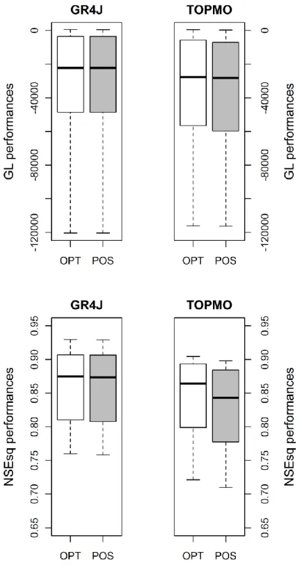
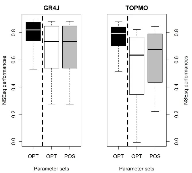
4.1 Calibration performance results
365
In this section, the general calibration performance of the two models are analysed. Figure 4 366
presents the distributions of the GL function evaluations and the distributions of the Nash-367
Sutcliffe efficiencies computed on root square transformed flows (NSEsq) obtained by the 368
GR4J and TOPMO models on the catchment set. The distributions were obtained with (i) the 369
calibration efficiencies over the whole record without the dry validation sub-periods obtained 370
with optimal parameter sets, i.e. 89 values for each model (white boxplots, noted OPT) and 371
(ii) calibration performance over the same record periods obtained with the 2000 posterior 372
parameter sets identified for each of the 89 catchments, i.e. 178,000 values for each model 373
(grey boxplots, noted POS). The distributions of the GL objective function values highlight 374
that optimal parameter sets present similar general calibration efficiency to the calibration 375
efficiency obtained using the populations of posterior parameter sets. Considering populations 376
of posterior parameter sets thus adds a limited variability in terms of calibration performance 377
over the whole record periods (without dry validation sub-periods) for the two models. For 378
GR4J, the distributions of the NSEsq efficiencies similarly show that the optimal parameter 379
identified with the DREAM algorithm and with the GL objective function have similar 380
general performance as the posterior parameter sets. The performance losses when 381
considering populations of posterior parameter sets instead of optimal parameter sets are more 382
significant for TOPMO than for GR4J, with median NSEsq moving from 0.86 with optimal 383
parameter sets to 0.84 with posterior parameter sets. Calibration performance results for the 384
other calibration sub-periods (wet, mean and dry 3-year calibration sub-periods) show the 385
same general tendencies (not shown here). The difference between the two models might stem 386
from the number of free parameters, higher for TOPMO (six free parameters) than for GR4J 387
(four free parameters). Thus, the calibrated parameter values of TOPMO may show greater 388
sensitivity to the choice of the objective function. Finally, note that the general performance 389
of both models is quite reasonable, with half of the catchments studied presenting calibration 390
performance obtained with optimal parameter sets on the whole record periods (without the 391
dry validation sub-periods) greater than 0.85 for the two models. 392
393
FIGURE 4: Distributions of the GL objective function values (top) and of the NSEsq values
394
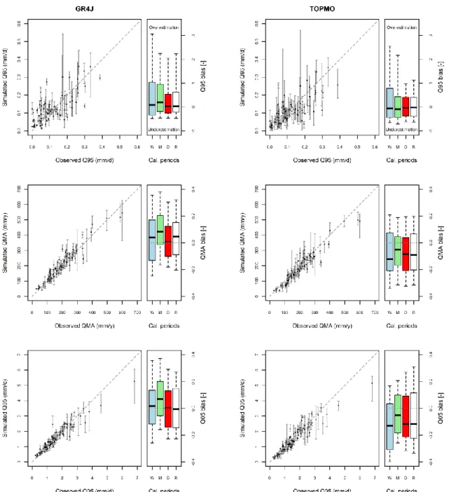
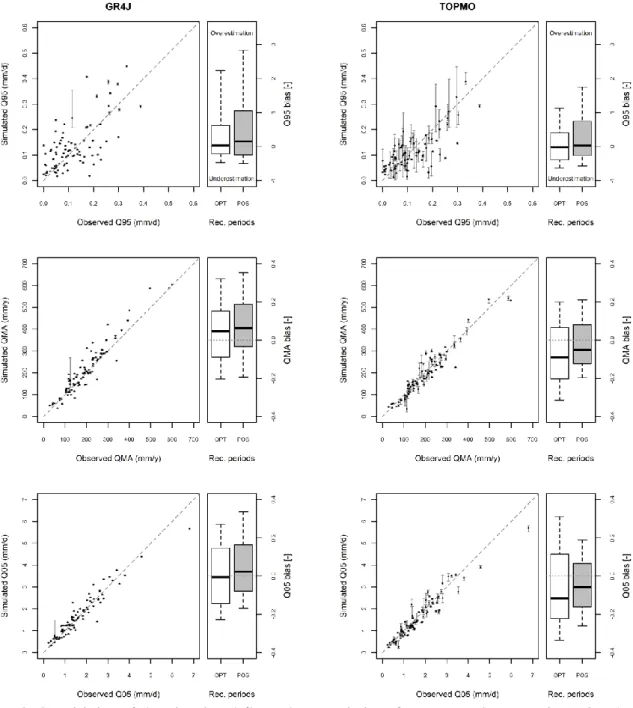
(bottom) of the two models illustrating (i) calibration performance over the whole record
395
periods without the dry validation sub-periods obtained with optimal parameter sets (white
396
boxplots, noted OPT) and (ii) calibration performance over the whole record periods
397
obtained with posterior parameter sets (grey boxplots, noted POS). Results are shown for
398
GR4J (left) and TOPMO (right). The boxplots show the 0.10, 0.25, 0.50, 0.75 and 0.90
399
percentiles.
400
4.2 Sensitivity to the climate characteristics of the calibration period
402
In this section, the model outputs are analysed considering different calibration periods. First 403
the efficiency of the model on the dry validation sub-periods is discussed in terms of NSEsq 404
and simulation of standard streamflow characteristics. Second, we analyse the resulting spread 405
of the simulated streamflows for the future time slices. 406
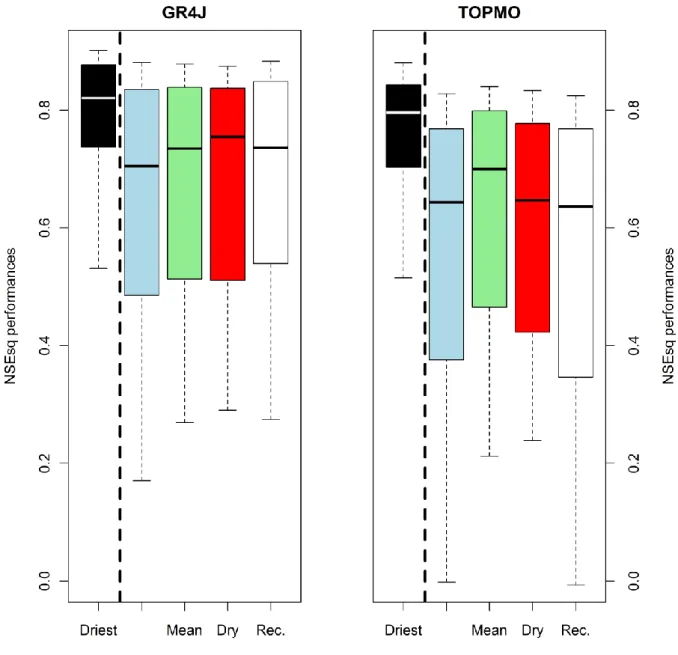
Efficiency on dry validation sub-periods: 407
Figure 5 shows the distributions of the NSEsq values on the catchment set obtained by the 408
two models in (i) calibration over the dry validation sub-periods and (ii) validation over the 409
dry validation sub-periods using the other four calibration sub-periods considered (wet, mean, 410
dry, and whole record periods). Models calibrated over different sub-periods generally 411
encountered similar difficulties simulating flows on the dry validation sub-periods since the 412
validation efficiencies are clearly reduced compared to the calibration efficiencies on this sub-413
period. The differences between the four calibration strategies (over a wet, a mean, a dry sub-414
period or a long period) are limited but, for both models, using the wettest sub-periods for 415
calibration appears particularly detrimental to simulating the dry validation sub-periods. GR4J 416
and TOPMO obtained marginally better validation results using dry and mean conditions for 417
calibration, respectively. Interestingly, calibrating the models on the whole record period 418
(except the dry validation sub-periods, resulting in 20 years of record on average) does not 419
warrant a particularly robust estimation of optimal parameter sets, since the validation 420
efficiencies are generally similar to those obtained with 3-year calibration periods. This is not 421
consistent with the wide-spread idea that the longer the calibration period, the more robust the 422
parameter set. 423
These results corroborate the previous findings of Vaze et al. (2010), Merz et al. (2011) and 424
Coron et al. (2012) obtained with different catchments and models, emphasising the lack of 425
robustness of conceptual rainfall-runoff models when the climatic settings between calibration 426
and validation periods are different. 427
428
FIGURE 5: Distributions of the NSEsq values obtained by the two models illustrating (i)
429
calibration performance over the dry validation sub-periods (black boxplots) and (ii)
430
validation performance over the dry validation sub-periods using the other four calibration
431
periods considered (wet, mean, dry, and whole record without the dry validation
sub-432
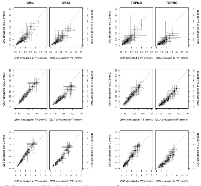
period illustrated, respectively, with blue, green, red and white boxplots). Results are shown
433
for GR4J (left) and TOPMO (right). The boxplots show the 0.10, 0.25, 0.50, 0.75 and 0.90
434
percentiles.
435
436
Figure 6 summarises the results of the models' sensitivity to the climatic specificity of the 437
calibration period on the observed dry validation sub-periods. This figure is organised as a 438
table with two columns and three rows: each column represents a hydrological model (left: 439
GR4J; right: TOPMO) and each row represents a specific characteristic of the simulated flow 440
series (from top to bottom: Q95, QMA and Q05). For each model and for each streamflow
441
characteristic, the plot on the left shows the observed versus simulated value for each 442
catchment, each dot representing the mean of simulated values obtained with the four optimal 443
parameter sets and each bar representing the range of simulated values when using the four 444
optimal parameter sets. Ideally, all range bars should be centred on the 1:1 line, meaning that 445
streamflow simulated by parameter sets originating from different calibration sub-periods are 446
all equal to the observed streamflow. The boxplots on the right represent the distributions of 447
the relative errors on the flow characteristic on the dry validation sub-periods over the 89 448
catchments when considering the four calibration sub-periods. These relative errors were 449
estimated as the ratio of the difference between simulated and observed flow characteristics to 450
the observed flow characteristics. Ideally, all the boxplots should be centred on a null value of 451
the bias between the observed and the simulated streamflow. 452
The first main result is that the two rainfall-runoff models present similar overall efficiency in 453
simulating the flow characteristics on the dry validation sub-periods (graphs on the left). This 454
efficiency is rather limited since the median absolute bias is greater than 0.1 for both models. 455
Even for the estimation of mean annual flow (QMA), none of the four calibration strategies
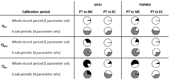
456
yields a median absolute bias lower than 0.1. The second main result is that the impact of the 457
climatic specificity of the calibration sub-periods on the modelled flow characteristics is not 458
straightforward (graphs on the right). For GR4J, it seems that the 3-year dry calibration sub-459
periods provide the least biased estimations of the three streamflow characteristics of the dry 460
validation sub-periods. Using wet and mean 3-year calibration sub-periods tends to yield 461
overestimated flow simulations on the dry validation sub-periods. Conversely, TOPMO tends 462
to underestimate flows of the dry validation periods. The mean 3-year calibration sub-463
periods seems to provide less biased estimation of the streamflow characteristics on the dry 464
validation sub-periods. Finally, using 3-year calibration sub-periods (dry ones for GR4J and 465
mean ones for TOPMO) yields less biased predictions than when considering the whole 466
available records for calibration for both hydrological models and for the three streamflow 467
characteristics studied here, which corroborates the validation performance illustrated in 468
Figure 5. Note, however, that all calibration periods produce highly biased predictions and 469
that the differences between the calibration strategies are relatively limited compared to these 470
biases. 471
472
FIGURE 6: Sensitivity of the simulated flow characteristics (from top to bottom: Q95, QMA
473
and Q05) on the dry validation sub-periods after calibration on climatically specific periods
474
(wet, mean, dry, total record) (left column: GR4J; right column: TOPMO). The Q-Q plots
show the observed versus simulated value for each catchment, each dot representing the mean
476
of values simulated with the four optimal parameter sets and each bar representing the range
477
of simulated values when using the four optimal parameter sets. The boxplots on the right
478
represent the distributions of the relative errors on the flow characteristic on the dry
479
validation sub-periods over the 89 catchments when considering the four calibration periods.
480
The boxplots are constructed with the 0.10, 0.25, 0.50, 0.75 and 0.90 percentiles.
481
482
Impacts on simulated flow evolutions: 483
Then we assessed the change in future simulated streamflow characteristics when considering 484
the variability stemming from the climatic specificity of the calibration periods. Figure 7 485
shows the models‟ outputs on future time slices when using the sets of model parameters 486
obtained on the four different calibration periods considered so far. The range of streamflow 487
characteristics simulated for future time slices (mid-century (MC) and end-of-century (EC)) 488
with the four parameter sets are plotted against those simulated for the present time slice (PT). 489
In the following, we assume that a model simulates a significant hydrological change on a 490
catchment if the range bar is completely above or below the 1:1 line, meaning that the change 491
can be considered beyond the variability generated by the climate specificity of the calibration 492
periods considered. For example, a decreasing trend of Q05 between PT and MC is assumed
493
for a particular catchment if a model calibrated over the four different sub-periods simulates 494
four Q05 values lower in MC than in PT.
495
Considering the range across centres, the two models suggest a rather similar decreasing trend 496
for the values of the three streamflow characteristics from PT to EC. This trend is not 497
observed for the MC time slice. The Q05 streamflow characteristic (high flows) increases for
498
this time slice, before decreasing more sharply by the end of the century. Some catchments 499
show particularly large range bars. An analysis of these catchments (not shown here) indicates 500
that the calibration performance is particularly poor for at least one calibration sub-period. 501
This shows that a model with poor performance in current conditions will add substantial 502
uncertainty to future predictions. 503
504
FIGURE 7: Comparison of the simulations of three streamflow characteristics (from top to
505
bottom: Q95, QMA and Q05) obtained on the present time slice (PT) and future time slices (MC
506
and EC) under projected climate conditions with the two hydrological models (left: GR4J;
507
right: TOPMO). The range bars represent, for each catchment, the range of estimated values
508
with the four optimal parameter sets corresponding to the four calibration periods.
509
510
The sensitivity of the two models to the climatic specificity of the calibration periods is of the 511
same magnitude for all three time slices considered, meaning that the sensitivity to the 512
calibration periods is relatively stable in the future time slices. Figure 8 synthesises the results 513
of these trends (e.g. a decreasing trend of Q05 between PT and MC is assumed for a particular
514
catchment when a model calibrated over the four different sub-periods simulates four Q05
515
values lower in MC than in PT), showing the proportion of catchments where hydrological 516
trends between present (PT) and future (MC and EC) time slices have been simulated 517
considering different calibration sub-periods for the two hydrological models. It also 518
compares the information given by a hydrological model calibrated over a long period (here 519
the entire available record without the dry validation sub-periods) and the information given 520
using the four different calibration periods. These results confirm the previously obtained 521
general trend of a decrease in the three streamflow characteristic values from PT to EC, with a 522
particular increasing trend for high flows (Q05) from PT to MC. Nevertheless, when
523
considering the four different calibration periods, a number of catchments show no clear 524
trends for the MC time slice, which attenuates the general trends highlighted when using the 525
whole record periods as the only calibration periods. Last, differences between the two 526
models can be observed: when considering only the whole record for calibration, GR4J seems 527
to simulate a more regionally homogeneous decrease in low- to medium-flow characteristics 528
(Q95 and QMA), since the percentage of catchments with a decrease in flow is larger than for
529
TOPMO. Considering the four calibration periods, the two models yield more homogeneous 530
simulations for the catchment set. 531
532
FIGURE 8: Proportions of catchments showing (or not) hydrological trends between present
533
(PT) and future (MC and EC) time slices considering different calibration sub-periods for the
534
two hydrological models: white highlights a clear decrease, black highlights a clear increase
535
and grey highlights no clear trend.
536
537
4.3 Sensitivity to the use of a posterior ensemble of parameter sets
538
In this section, the model outputs are analysed considering 2000 posterior parameter sets 539
obtained on the whole record period for each catchment and for each model. First, we discuss 540
the efficiency of these ensembles of posterior parameter sets on the dry validation sub-periods 541
in terms of NSEsq and simulation of the three streamflow characteristics (Q95, QMA and Q05).
542
Second, we analyse the resulting variability of the simulated streamflow characteristics for the 543
future climate conditions. 544
Efficiency on dry validation sub-periods: 545
Figure 9 shows the distribution of NSEsq values obtained by the two models illustrating (i) 546
the calibration performance of the optimal parameter sets over the dry validation sub-periods 547
(i.e. 89 NSEsq values for each model) and (ii) the validation performance over the dry 548
validation sub-periods using optimal parameter sets (i.e. 89 NSEsq values for each model) and 549
posterior parameter sets (i.e. 178,000 NSEsq values for each model) identified on the whole 550
record periods without the dry validation sub-periods. For GR4J, the validation performance 551
obtained by posterior parameter sets is very similar to that produced by the individual optimal 552
parameter sets presented in Figure 5, meaning that for the catchments studied, the DREAM 553
algorithm produces posterior parameter sets yielding efficiency close to the value obtained by 554
optimal parameter sets over the dry validation sub-periods. The NSEsq performance 555
distributions obtained with optimal and posterior parameter sets are not similar for TOPMO: 556
the optimal parameter sets appear to be less efficient than the posterior parameter sets in terms 557
of NSEsq validation performance. This means that rather different optima exist when using 558
the GL function and a likelihood function based on a standard least squares errors scheme 559
(NSEsq here). Nevertheless, differences between optimal parameter set performance and 560
posterior parameter set performance are less significant in the validation step than in the 561
calibration step, as shown in Figure 4. It should be remembered that the NSEsq was not used 562
as an objective function. 563
564
FIGURE 9: Distribution of NSEsq values obtained by the two models illustrating (i)
565
calibration performance of the optimal parameter sets over the dry-validation sub-periods
566
(black “OPT” boxplots) and (ii) validation performance over the dry validation sub-periods
567
using optimal (white “OPT” boxplots) and posterior (grey “POS” boxplots) parameter sets
568
identified on the whole record periods without the dry validation sub-periods. Results are
569
shown for GR4J (left) and TOPMO (right). The boxplots show the 0.10, 0.25, 0.50, 0.75 and
570
0.90.
571
572
Figure 10 shows the variability of the models‟ outputs on the dry validation sub-periods when 573
considering the ensembles of posterior parameter sets instead of the single optimal parameter 574
set. This figure is organised like Figure 6. The dots represent the means of flow characteristics 575
on a catchment simulated with the 2000 posterior parameter sets and the bars represent the 576
range of simulated flow characteristics on a catchment when considering its 2000 posterior 577
parameter sets. The boxplots synthesise the distributions of the relative errors on the flow 578
characteristics simulated by the models with the posterior parameter sets identified. 579
The first major result is that considering posterior parameter sets does not significantly 580
increase the variability of the simulated flows. The biases between observed flows and flows 581
simulated by the ensembles of posterior parameter sets (grey boxplots) are close to those 582
obtained with the ensembles of optimal parameter sets (white boxplots). Moreover, this 583
variability is very limited compared to the variability observed when considering the four 584
climate-specific parameter sets (see Figure 6). Here, the hydrological responses associated 585
with 2000 posterior parameter sets are similar to those associated with optimal parameter sets. 586
The flow characteristics obtained by TOPMO present generally greater uncertainty than those 587
obtained by GR4J. These predictive uncertainty values are again probably due to the larger 588
number of free parameters for TOPMO. Note, however, that the predictive uncertainty for 589
TOPMO is often consistent with the observed biases for the validation sub-periods since the 590
estimation range often encompasses the observed flow value. 591
592
FIGURE 10: Sensitivity of the simulated flow characteristics (from top to bottom: Q95, QMA
593
and Q05) on the dry validation sub-periods using the 2000 posterior parameter sets
594
determined on the whole record periods without the dry validation sub-periods for the two
595
hydrological models (left: GR4J; right: TOPMO). The Q-Q plots show the observed versus
596
simulated value for each catchment, each dot representing the mean of simulated values when
597
using the 2000 posterior parameter sets and each bar representing the range of simulated
598
values when using the 2000 posterior parameter sets. The boxplots on the right represent the
599
distributions of the relative errors on the flow characteristic on the dry validation sub-periods
over the 89 catchments when considering the 2000 posterior parameter sets. The boxplots are
601
constructed with the 0.10, 0.25, 0.50, 0.75 and 0.90 percentiles.
602
603
Impacts on simulated flow evolutions: 604
Figure 11 synthesises the results on the evolution of flows when considering the posterior 605
parameter sets obtained throughout the whole record periods. This figure is organised like 606
Figure 7: for each catchment, a range cross quantifies the variability in the estimation of flow 607
characteristics for a time slice simulated by the posterior parameter sets obtained on the whole 608
record periods. The results are very different from those obtained when considering only the 609
individual optimal parameter sets for each of the four calibration periods (Figure 7). The 610
variability of simulated flows considering 2000 posterior parameter sets for each catchment is 611
much lower than the variability considering four climate-specific parameter sets for each 612
catchment. Nevertheless, the variability in TOPMO outputs considering posterior parameter 613
sets is higher than GR4J‟s variability. 614
615
FIGURE 11: Comparison of the simulations of three streamflow characteristics (from top to
616
bottom: Q95, QMA and Q05) obtained on the present time slice (PT) and future time slices (MC
617
and EC) under projected climate conditions with the two hydrological models (left: GR4J;
618
right: TOPMO). For each catchment, the range bars represent the range of estimated values
619
with the 2000 posterior parameter sets obtained over the whole record period.
620
621
Figure 12 illustrates the proportion of catchments showing (or not showing) clear changes 622
when considering the ensemble simulations obtained with the posterior parameter sets. The 623
additional consideration of the ensembles of 2000 posterior parameter sets yields a slight 624
increase in the number of catchments for which no clear trend is observed, particularly 625
between the MC and the PT. Nevertheless, the future trends are similar to those observed 626
without taking into account the ensembles of posterior parameter sets, i.e. when using only the 627
optimal parameter sets. There is a sharp decrease in all streamflow characteristics by the EC 628
and a slight but significant increase in the high-flow characteristic for the MC. 629
630
FIGURE 12: Proportion of catchments showing (or not showing) hydrological trends
631
between present (PT) and future (MC and EC) time slices considering (or not considering)
632
posterior parameter sets for the two hydrological models: white highlights a clear decrease,
633
black highlights a clear increase and grey highlights no clear trend.
634
635
5 DISCUSSION AND CONCLUSION
636
This paper attempted to investigate the uncertainty of hydrological predictions for the future 637
climate when considering either (i) the dependence of the optimal parameter set on calibration 638
period specificity or (ii) the use of several posterior parameter sets over a given calibration 639
period. The first aspect often refers to the robustness of model parameters, while the second 640
often refers to parameter uncertainty estimation based on Bayesian inference. 641
The two conceptual hydrological models tested here were sensitive to the use of climatically 642
contrasted calibration sub-periods. This sensitivity was highlighted by a wide range of 643
possible simulated streamflows for both the dry observed validation sub-periods and the 644
future climate time slices. Even if general future changes can be observed when considering 645
four optimal parameter sets (obtained with the calibration on three sub-periods and the whole 646
record periods except the dry validation sub-periods) for each catchment, the proportion of 647
catchments showing clear changes is much lower than when considering a unique parameter 648
set (obtained by calibration on the whole record periods except the dry validation sub-649
periods). However, the impact of the calibration period climate specificity on the simulated 650
streamflows is not straightforward since for a majority of the catchments studied, using a wet 651
calibration sub-period for a dry validation sub-period does not systematically generate a larger 652
bias between observed and simulated flows than when using a dry calibration sub-period. 653
Moreover, considering long periods for model calibration does not generate more robust 654
simulation than using 3-year sub-periods, which is not consistent with the common belief that 655
“the longer the calibration period, the more robust the parameter set”. Since the use of two 656
different hydrological models did not provide equivalent results, the relation between the 657
model considered and the impact of the climatic specificity of the calibration period on 658
calibration and validation performance should be further investigated. 659
Concerning the “classical” parameter uncertainty assessment followed in this study, it seems 660
that the prediction bounds obtained from the ensembles of posterior parameter sets are 661
considerably thinner than what would be expected, especially for the GR4J model. 662
Nevertheless, it is important to note that these results are dependent to some extent on the 663
method used (the DREAM algorithm (Vrugt et al., 2009) and the GL objective function 664
(Schoups and Vrugt, 2010)), the catchments studied and the models considered. It appeared 665
that DREAM provided posterior parameter sets that were close to the optimal ones in terms of 666
Nash-Sutcliffe validation efficiency over the dry validation sub-periods. Other methods to 667
quantify parameter uncertainty could produce posterior parameter sets with greater 668
differences than the optimal ones and thus yield larger uncertainty bounds. Considering the 669
ensembles of 2000 posterior parameter sets yields a slight increase in the number of 670
catchments for which no clear trend is observed, especially for TOPMO. The results obtained 671
by the two conceptual models were found to be relatively consistent. The main differences 672
were the larger uncertainty bounds observed for TOPMO. This is probably attributable to the 673
larger number of degrees of freedom of TOPMO, which has six free parameters, compared to 674
the four free parameters of GR4J. TOPMO‟s calibrated parameters are thus likely to depend 675
more on the choice of the calibration period and the objective function used during the 676
optimisation process. Still, further research is needed to confirm these hypotheses. 677
Our results show that, given the evaluation approach followed here, model robustness was the 678
major source of variability in streamflow projections in future climate conditions. They 679
corroborate the previous findings of Vaze et al. (2010), Merz et al. (2011) and Coron et al. 680
(2012) obtained with different catchment sets and models, emphasising the lack of robustness 681
of conceptual rainfall-runoff models when the climatic context between calibration and 682
validation periods are different. Note that for these three studies, long-term regional non-683
stationarities were observed on the catchments studied: southeastern Australian catchments 684
suffered from long drought periods while Austrian catchments experienced a significant 685
increase in temperature over the last few decades, generating a shift in the hydrological 686
regimes, particularly for snow-affected catchments. These situations allow testing the 687
hydrological models on long as well as significantly different sub-periods in terms of climatic 688
conditions. Even if these actual non-stationarities were not observed everywhere, it seems 689
possible to test the sensitivity of models‟ calibration on climatically contrasted sub-periods. 690
Thus, from these results, it seems difficult to provide general guidelines for calibrating 691
hydrological models for climate change studies. The robustness issue should be investigated 692
more thoroughly, by proposing and testing calibration procedures that increase this 693
robustness. For example, Coron et al. (2012) proposed the Generalized Split Sample Test 694
procedure, which aims at testing all possible combinations of calibration-validation periods 695
and thus studying the capability of the tested model to be used in different climatic contexts. 696
Other tests could be performed, inspired by the methodology defined in this work. 697
This study also stresses that hydrological models do not efficiently reproduce streamflow 698
characteristics, even if the NSEsq coefficient estimated after calibration is quite high. The 699
median bias obtained for mean annual flow was generally greater than 10%. This is a 700
considerable limitation for the use of hydrological models to simulate extreme high or low 701
flows in a changing climate. To cope with this notable failure, one could suggest using multi-702
objective calibration procedures and/or adapting the objective function to the estimated flow 703
characteristic. 704
706
6 ACKNOWLEDGMENTS
707
All hydro-meteorological data were provided by two research programs that addressed the 708
potential impacts of climate change: the RexHySS project (Ducharne et al., 2009; Ducharne et 709
al. 2011) on the Seine and the Somme basins and the ICC-Hydroqual (Moatar et al., 2010) 710
project on the Loire basin. 711
The authors thank the reviewers who provided constructive comments on an earlier version of 712
the manuscript, which helped clarify the text. Among them, Jasper Vrugt is thanked for 713
providing the codes to implement the optimisation approach he advised. Finally, François 714
Bourgin (IRSTEA) is also acknowledged for his comments and suggestions. 715