HAL Id: hal-01945345
https://hal.inria.fr/hal-01945345
Submitted on 5 Dec 2018
HAL is a multi-disciplinary open access archive for the deposit and dissemination of sci-entific research documents, whether they are pub-lished or not. The documents may come from teaching and research institutions in France or abroad, or from public or private research centers.
L’archive ouverte pluridisciplinaire HAL, est destinée au dépôt et à la diffusion de documents scientifiques de niveau recherche, publiés ou non, émanant des établissements d’enseignement et de recherche français ou étrangers, des laboratoires publics ou privés.
Estefania Cano, Derry Fitzgerald, Antoine Liutkus, Mark Plumbley,
Fabian-Robert Stöter
To cite this version:
Estefania Cano, Derry Fitzgerald, Antoine Liutkus, Mark Plumbley, Fabian-Robert Stöter. Musical Source Separation: An Introduction. IEEE Signal Processing Magazine, Institute of Electrical and Electronics Engineers, 2019, 36 (1), pp.31-40. �10.1109/MSP.2018.2874719�. �hal-01945345�
Musical Source Separation: An Introduction
Estefanía Cano, Derry FitzGerald, Antoine Liutkus, Mark D. Plumbley, Fabian-Robert Stöter
I. INTRODUCTION
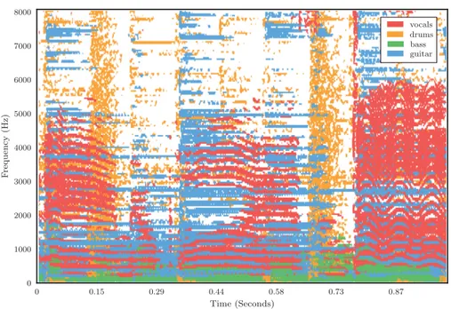
Figure 1: Representation of a music mixture in the time-frequency domain. The dominant musical source in each time-frequency bin is displayed with a different color.
Many people listen to recorded music as part of their everyday lives, for example from radio or TV programmes, CDs, downloads or increasingly from online streaming services. Sometimes we might want to remix the balance within the music, perhaps to make the vocals louder or to suppress an unwanted sound, or we might want to upmix a 2-channel stereo recording to a 5.1-channel surround sound system. We might also want to change the spatial location of a musical instrument within the mix. All of these applications are relatively straightforward, provided we have access to separate sound channels (stems) for each musical audio object.
However, if we only have access to the final recording mix, which is usually the case, this is much more challenging. To estimate the original musical sources, which would allow us to remix, suppress or upmix the sources, we need to perform musical source separation (MSS).
In the general source separation problem, we are given one or more mixture signals that contain different mixtures of some original source signals. This is illustrated in Figure 1 where four sources, namely vocals, drums, bass and guitar, are all present in the mixture. The task is to recover one or more of the source signals given the mixtures. In some cases, this is relatively straightforward, for example, if there are at least as many mixtures as there are sources, and if the mixing process is fixed, with no delays, filters or non-linear mastering [1].
However, MSS is normally more challenging. Typically, there may be many musical instruments and voices in a 2-channel recording, and the sources have often been processed with the addition of filters and reverberation (sometimes nonlinear) in the recording and mixing process. In some cases, the sources may move, or the production parameters may change, meaning that the mixture is time-varying. All of these issues make MSS a very challenging problem.
Nevertheless, musical sound sources have particular properties and structures that can help us. For example, musical source signals often have a regular harmonic structure of frequencies at regular intervals, and can have frequency contours characteristic of each musical instrument. They may also repeat in particular temporal patterns based on the musical structure.
In this paper we will explore the MSS problem and introduce approaches to tackle it. We will begin by introducing characteristics of music signals, we will then give an introduction to MSS, and finally consider a range of MSS models. We will also discuss how to evaluate MSS approaches, and discuss limitations and directions for future research 1.
II. CHARACTERISTICS OF MUSIC SIGNALS
Music signals have distinct characteristics that clearly differentiate them from other types of audio signals such as speech or environmental sounds. These unique properties are often exploited when designing MSS methods, and so an understanding of these characteristics is crucial.
All music separation problems start with the definition of the desired musical source to be separated, often referred to as the target source. In principle, a musical source refers to a particular musical instrument, such as a saxophone or a guitar, that we wish to extract from the audio
1 A dedicated website with complementary information about MSS including sound examples, an extended
bibliography, dataset information, and accompanying code can be reached on the following link: https://soundseparation. songquito.com/
mixture. In practice, the definition of musical source is often more relaxed, and can refer to a group of musical instruments with similar characteristics that we want to separate. This is the case, for example, in singing voice separation, where the goal often includes the separation of both the main and background vocals from the mixture. In some cases, the definition of musical source can be even looser, as is the case in harmonic-percussion separation, where the aim is to separate the pitched instruments from the percussive ones.
In a general sense, musical sources are often categorized as either predominantly harmonic, predominantly percussive, or as singing voice. Harmonic music sources mainly contain tonal components, and as such, they are characterized by the pitch or pitches they produce over time. Harmonic signals exhibit a clear structure composed of a fundamental frequency F0 and a harmonic series. For most instruments, the harmonics appear at multiple integers of the fundamental frequency: for a given F0 at 300 Hz, a harmonic component can be expected close to 600 Hz, the next harmonic around 900 Hz, and so on. Nonetheless, a certain degree of inharmonicity, i.e., deviation of harmonics from multiple integers of F0, should be expected and
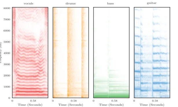
Figure 2: Magnitude spectrogram of four example music signals: vocals (left), drums (mid-left), bass (mid-right) and acoustic guitar (right). The horizontal axis represents time in seconds, and
accounted for. Harmonic sources exhibit a relatively stable behavior over time, and can typically be identified in the spectrogram as horizontal components. This can be observed in Figure 2 where a series of notes played by an acoustic guitar are displayed. Additionally, the trajectories in time of the F0 and the harmonics are usually very similar, a phenomenon referred to as common fate [2]. This can be clearly seen in the spectrogram of the vocals in Figure 2, where it can be observed that the vocal harmonics have common trajectories over time. The relative strengths of the harmonics, and the way that the harmonics evolve over time, contribute to the characteristic sound, or timbre, which allows the listener to differentiate one instrument from another. Furthermore, and particularly in Western music, the sources often play in harmony, where the ratios of the F0s of the notes are close to integer ratios. While harmony can result in homogeneous and pleasing sounds, it most often also implies a large degree of overlap in the frequency content of the sources, which makes separation more challenging.
In contrast to harmonic signals, which contain only a selected number of harmonic components, percussive signals contain energy in a wide range of frequencies. Percussive signals exhibit a much flatter spectrum, and are highly localized in time with transient-like characteristics. This can be observed in the drums spectrogram in Figure 2, where clear vertical structures produced by the drums signal can be observed. Percussive instruments play a very important role of conveying rhythmic information in music, giving a sense of speed or tempo in a musical piece.
In reality, most music signals contain both harmonic and percussive elements. For example, a note produced by a piano is considered predominantly harmonic, but it also contains a percus-sive attack produced by the hammer hitting the strings. Similarly, singing voice is an intricate combination of harmonic (voiced) components, produced by the vibrations of the vocal chords, and percussive-like (plosive) components including consonant sounds such as ‘k’ or ‘p’ where no vocal fold vibration occurs. These components are in turn filtered by the vocal cavity, with different formant frequencies created by changing the shape of the vocal cavity. As seen in Figure 2, singing voice typically exhibits a higher rate of pitch fluctuation compared to other musical instruments.
A notable property of musical sources is that they are typically sparse in the sense that for the majority of points in time and frequency, the sources have very little energy present. This is commonly exploited in MSS, and can be clearly seen for each of the sources in Figure 2. Another characteristic of music signals is the fact that music signals typically exhibit repeating structures over different time-scales, for example, a repeating percussion pattern over a couple
Hardware
Effects InterfaceAudio DAW StereoTrack
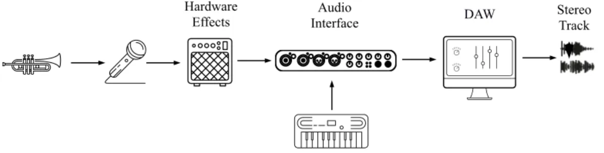
Figure 3: Common music recording and mixing setup. In most cases, musical content is combined and mixed into a stereo signal using a Digital Audio Workstation (DAW).
of seconds, to larger structures such as the verse-chorus structures found in pop songs. As will be explained in Section IV-B, these repetitions can be leveraged when performing MSS.
The bulk of research on MSS to-date has focused on Western pop music as the main genre to be separated. It should be noted that other types of music present their own unique problems for MSS, for example, many instruments playing in unison in some types of traditional/folk music. These cases are typically not covered by existing MSS techniques.
Once the target source has been defined, the characteristics of the audio mixture should be carefully considered when developing MSS methods. Modern music production techniques offer innumerable possibilities for transforming and shaping an audio mix. Most music signals nowadays are created using audio content from a great diversity of origins, usually combined and mixed using a Digital Audio Workstation (DAW), a software system for transforming and manipulating audio tracks. As depicted in Figure 3 for the trumpet, some musical sources can be recorded in a traditional manner using a microphone or a set of microphones. Very often, hardware devices that shape and color the sound are introduced into the signal chain; these may include, for example, guitar tube amplifiers or distortion pedals which can impart very particular sound qualities to the signal. In other cases, musical sources are not captured using a microphone. Instead, the digital signal they produce is directly fed into the DAW, or alternatively created within the system itself, using, for example, a keyboard as an interface as shown in Figure 3 Most frequently, an audio interface is used to facilitate the process of capturing input signals from different origins, and delivering them to the DAW. The DAW itself offers many additional possibilities to further enhance and modify the signal.
commercial music today is in stereo format (2 channels). Other multi-channel formats such as 5.1 (5 main channels plus a low frequency channel) are available but less common. The number of channels available to perform music separation is a key factor that can be exploited when designing MSS models. Multichannel mixtures allow spatial positioning of the music sources in the sound field. This means that a certain source can be perceived as coming from the left, the center, the right or somewhere in between. The spatial positioning of the sources is usually achieved with a pan pot that regulates the contribution of each musical source in each of the available channels. This artificial creation of spatial positioning ignores delay as a spatial cue, and so inter-channel delay is much less important in MSS than in speech source separation. In contrast, monophonic (single channel) recordings offer no information about spatial positioning, and are often the most challenging separation problem.
A final but fundamental aspect to be considered when designing MSS systems is the fact that music quality, and audio quality in general, is inherently defined and measured by human perception. This sets an additional challenge to MSS methods: regardless of the mathematical soundness of the model, all systems are expected to result in perceptually pleasing music signals. Aside from the task of truthfully capturing the target source, we must also minimize the impact on perceptual quality of the distortions introduced in the separation process.
III. A TYPICALMUSICALSOURCESEPARATION WORK FLOW
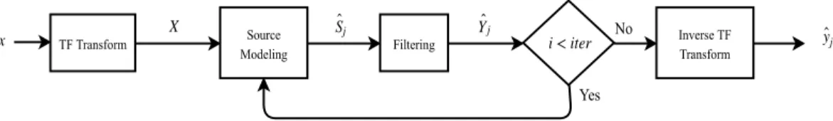
A high-level overview of the steps involved in most MSS systems is illustrated in Figure 4. First the input mixture signal is transformed to the time-frequency (TF) domain. The TF representation of the signal is then manipulated to obtain parameters which model the individual sources in the mixture. These are then used to create filters to yield time-frequency estimates of the sources. This is typically done in an iterative manner before the final estimated time-domain signals are recovered via an inverse time-frequency transform. To describe these steps in greater detail, we first introduce the mathematical notation used.
Notation: Musical source separation involves decomposing a time-domain audio mixture signal x into its constituent musical sources yj. Both x and yj are vectors of samples in time. Here,
the index j denotes the musical source, with j ∈ {1 · · · J } and J the total number of sources in the mixture. Time-frequency (TF) representations are denoted in uppercase, with X denoting the complex spectrogram of the mixture x, and Yj the complex spectrogram of the source yj.
Round brackets are used to denote individual elements in a time frequency representation, with frequency bins denoted with k and time frames with n. The magnitude spectrogram of source
TF Transform Source
Modeling Filtering
Inverse TF Transform
x X Ŝ j Ŷ j i < iter ŷ j
Yes No
Figure 4: Common MSS work flow: source models are obtained from the spectrogram of the audio mix. This is often done in an iterative manner where iter represents the total number of
iterations and i the iteration index.
j is defined as Sj = |Yj|, while ˆYj, ˆSj and ˆyj denote estimates of the source time frequency
representation, magnitude spectrogram, and source signal, respectively.
Time-Frequency (TF) Transformation: Most research in MSS has focused on the use of the Short-Time Fourier Transform (STFT), X (k, n) ∈ C. The complex STFT has the advantage of being computationally efficient, invertible and linear: the mixture equals the sum of the sources in the transformed domain, X =P
jYj. Other transform alternatives like the Constant Q transform
have been proposed, but have not, as yet, found widespread use in MSS.
Source Modeling: Most MSS methods focus solely on analyzing the magnitude spectrogram M = |X| of the mix. The goal at this stage is to estimate either a model of the spectrogram of the target source, or a model of the location of the target source in the sound field. As will be explained in Section IV, source models and spatial models are the most common approaches used for MSS. In Figure 4, an example is presented where starting with the mixture X, estimates of the magnitude spectrograms of the sources ˆSj are obtained.
Filtering: The goal at this stage is to estimate the separated music source signals given the source models. This is typically done using a soft-masking approach, the most common form of which is the Generalized Wiener Filter (GWF) [3], though other soft-masking approaches have been used [4]. Given X and ˆSj, this allows recovery of the separated sources provided
their characteristics are well estimated. The STFT of source j = 1 can be estimated elementwise using the GWF as ˆY1(k, n) = X(k, n) ˆS1(k, n)/PjSˆj(k, n). The same procedure is applied for
all sources in the mix. Essentially, each time-frequency point in the original mixture is weighted with the ratio of the source magnitude to the sum of the magnitudes of all sources. This can be understood as a multi-band equalizer of hundreds of bands, changed dynamically every few milliseconds to attenuate or let pass the required frequencies for the desired source. A special
case of the Generalized Wiener Filter is the process of binary masking, where it is assumed that only one source has energy at a given time-frequency bin, so that masks values are either 0 or 1. Estimating source parameters from the mixture is not trivial, and it can be difficult to obtain good source parameters to enable successful filtering at the first try. For this reason, it is common to proceed iteratively: First, separation is achieved with the current estimated source models. These models are then updated from the separated signals, and the process repeated as necessary. This approach is illustrated in Figure 4 and rooted in the Expectation-Maximization algorithm. Most of the models presented in Section IV may be used in this iterative methodology.
Inverse Transform: The final stage in the MSS work flow is to obtain the time domain source waveforms yj using the inverse transform of the chosen time frequency representation.
IV. MUSICALSOURCESEPARATIONMODELS
Having described the necessary steps for MSS, we now focus on how the unique characteristics of musical signals are used to perform MSS. While numerous categorizations of MSS algorithms are possible, such as categorization by source type, here we take the approach of dividing the algorithms into two broad categories: algorithms which model the musical sources, and those which model the position of the sources in multichannel or stereo audio signals. The key distinction between these two categories is that algorithms in the first category model aspects of the mixture intrinsic to the sources, while those in the second category model aspects intrinsic to the recording/mixing process. Models in the two categories exploit distinct but complementary information which can readily be combined to yield more powerful MSS models.
A. Musical Source Position Models
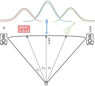
In the case of multichannel music signals, the spatial position of the sources has often been exploited to perform music source separation. In this section, we assume that we are dealing with a stereo (2-channel) mixture signal, and that the spatial positioning of source j has been achieved using a constant power panning law, defined by a single parameter, the panning angle φj ∈ [0, π/2]. For a given source qj, its stereo representation (or stereo image) is given by
y1j = qjcosθj and y2j = qjsinθj, with the subscripts 1 and 2 explicitly denoting the first and
second channels, respectively. Figure 5 illustrates the spatial positioning of three sources. The singing voice, for example, is positioned in the center and hence, its stereo image is obtained with an angle of π/4.
Figure 5: Illustration of standard Pan Law. The position of the source j = 1 (keyboard), source j = 2 (voice), and source j = 3 (guitar) is defined by the angle φj which is always measured
with respect to the first channel. Also shown are individual (colored) source position histograms and the mixture spatial histogram (black)
One of the earliest techniques used to exploit spatial position for MSS was Independent Component Analysis (ICA) [1], which estimates an unmixing matrix for the mixture signals based on statistical independence of the sources. However, ICA requires mixtures that contain the same number of channels as musical sources in the mix. This is not typically the case for music signals, where there are usually more sources than channels.
As a result of the shortcomings of ICA, algorithms which worked when there were more sources than channels were developed. Several techniques utilizing spatial position for separation, such as DUET [5], ADRess [6], and PROJET [7], assume that the time-frequency representations of the sources have very little overlap. This assumption, which holds to a surprising degree for speech, does not hold entirely for music, where the use of harmony and percussion instruments ensures there is overlap. Nonetheless, this assumption has proved to be useful in many circumstances, and often results in fast algorithms capable of real-time separation. The degree of overlap between sources can be seen, for example, in the spectrogram shown in Figure 1 which only shows the
dominant musical source in each time-frequency bin of the mixture.
To illustrate the usefulness of assuming very little overlap between sources, consider the element-wise ratio of the individual mixture channels in the time-frequency domain R(k, n) = |X1(k, n)/X2(k, n)|, where the subscript indicates channel number. If there is little time-frequency
overlap between the sources, then a single source j will contribute most of the energy at a single point in the time-frequency representations, and so R(k, n) ≈ cos φj/ sin φj. Given that R(k, n)
only depends on φj under this assumption, it can therefore be used to estimate a panning angle for
each time-frequency point. By plotting an energy-weighted histogram of these angle estimates, a mixture spatial histogram as the one shown in Figure 5 can be obtained. A peak in this histogram then provides an estimate of the panning angle φj of a given source. All time-frequency points
with an angle close to that of the jth peak are assigned to source j. Then, recovery of an estimate of source j can be done by means of binary masking. DUET, ADRess and PROJET all estimate histograms of energy vs angle. The main difference between the techniques lies in how these histograms are generated and used, and in the type of masking used. Both DUET and ADRess require peak picking from a mixture spatial histogram and use binary masking. PROJET estimates individual source position histograms, the superposition of which results in the mixture spatial position histogram (as shown in Figure 5). Further, PROJET utilizes the GWF for masking. It should also be noted that both DUET and PROJET can also incorporate and deal with inter-channel delays, extending their range of applicability.
The aforementioned separation methods directly model sound engineering techniques such as panning and delay for creating multichannel mixtures. Another line of research models the spatial configuration of a source directly through inter-channel correlations: At each frequency k, the correlation between the STFT coefficients of the different channels is calculated and encoded in a matrix called the spatial covariance matrix. The core idea of such methods is to leverage the correlations between channels to design better filters than those obtained by considering each channel in isolation. This approach is termed Local Gaussian Modeling (LGM) [3], [8]. It can give good separation whenever the spatial covariance matrices are well estimated for all sources. It is also able to handle highly reverberated signals, for which no single direction of arrival may be identifiable. This strength of covariance-based methods in dealing with reverberated signals comes at the price of difficult parameter inference. LGM algorithms are often very sensitive to initialization, and the estimated spatial covariance matrices alone are often not sufficient to allow separation. Successful LGM methods need to incorporate musical source models to further
guide the separation to obtain acceptable solutions. Musical source models are discussed in the following section.
B. Musical Source Models
While spatial positioning can give good results if each source occupies a unique stereo position, it is common for multiple sources to be located in the same stereo position, or for the mixture signal to consist of a single channel. In these cases, model-based approaches that attempt to capture the spectral characteristics of the target source can be used. In the following sections, a range of MSS model-based approaches are described.
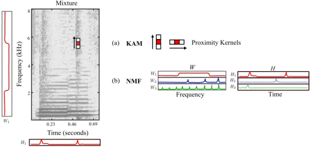
Kernel Models: Similarly to the idea that the definition of the target sources can be relatively loose in a MSS scenario (see Section II), source models can also incorporate different degrees of specificity when it comes to describing the sources in the mix. Consider for example the harmonic-percussive separation task: harmonic sources are characterized as horizontal components in the spectrogram, while percussive sources are characterized as time-localized vertical ones. These particularities of the sources can also be understood as harmonic sources exhibiting continuity over time, and percussive sources exhibiting continuity over frequency. Music separation models such as Kernel Additive Models (KAM) particularly exploit local features observable in music spectrograms such as continuity, repetition (at both short time scales and longer scales such as repeating verses and choruses) and common fate [9]. In order to estimate a music source at a given time-frequency point, KAM involves selecting a set of time-frequency bins, which, given the nature of the target source, e.g., percussive, harmonic or vocals, are likely to be similar in value. This set of time-frequency bins is termed a proximity kernel. An example of a vertical proximity kernel used to extract percussive sounds is shown in Figure 6a. Here, a set of adjacent frequency bins are chosen since percussion instruments tend to exhibit stable ridges across frequency. The vertical kernel is also positioned on a percussive hit seen in the spectrogram of the mixture in Figure 6, where the middle time-frequency bin (k, n) is the one to be estimated. In the case of sustained pitched sounds which tend to have similar values in adjacent time frames, a suitable proximity kernel consists of adjacent time-frames across a single frequency (see the horizontal kernel in Figure 6a). KAM approaches assume that interference due to other sources than the target source is sparse, so time-frequency bins with interference are regarded as outliers. To remove these outliers and to obtain an estimate of the target source, the median amplitude of the bins in the proximity kernel is taken as an estimate of the target source at a given time-frequency bin. The median acts as a statistical estimator robust to outliers in energy. Once the
KAM H W Proximity Kernels Time (a) NMF (b) Frequency Mixture Time (seconds) Frequency (kHz) 0.23 0.46 0.69 2 4 6 8
Figure 6: Example of different models used in MSS: (a) Proximity kernels used for harmonic-percussive separation within a Kernel Additive Modeling (KAM) approach, (b) Spectral templates W and time activations H within a Non-Negative Matrix Factorization
approach.
proximity kernels have been chosen for each of the sources to be separated, separation proceeds iteratively in the manner described in Section III. KAM is a generalization of previous work on vocal separation and harmonic-percussive separation [4], [10], and has demonstrated considerable utility for these purposes [9].
Spectrogram Factorization Models: Another group of musical source models are based on spectrogram factorization techniques. The most common of those is Non-Negative Matrix Factorization (NMF). NMF attempts to factorize a given negative matrix into two non-negative matrices [11]. For the purpose of musical source separation, NMF can be applied to the non-negative magnitude spectrogram of the mix M . The goal is to factorize M into a product M ≈ W H of a matrix of basis vectors W , which is a dictionary of spectral templates modeling spectral characteristics of the sources, and a matrix of time activations H. Figure 6b shows an example of a series of spectral templates and their corresponding time activations. One of the spectral templates W1, and its corresponding time activations H1, are also displayed next to the
mixture spectrogram. Peaks in the time activations represent the time instances where a given spectral template has been identified within the mix. Note, for example, that the peaks in the time activation H1 coincide with the percussive hits (vertical structures) in the spectrogram. The
factorization task is solved as an optimization problem where the divergence (or reconstruction error) between M and W H is minimized using common divergence measures D such Kullback-Leibler, or Itakura-Saito: minW,H≥0D(M kW H). Many variants of NMF algorithms have been
proposed for the purpose of musical source separation, including methods with temporal continu-ity constraints [12], multichannel separation models [8], score-informed separation [13], among others [14].
The NMF-based methods presented above typically assume that the spectrogram for all sources may be well approximated through low-rank assumptions, i.e. as the combination of only a few spectral templates. While this assumption is often sufficient for instrumental sounds, it generally falls short on modeling vocals, which typically exhibit great complexity and require more sophisticated models. In this respect, an NMF variant that has been particularly successful in separating the singing voice uses a source-filter model to represent the target vocals [15]. The idea behind such models is that the voice signal is produced by an excitation that depends on a fundamental frequency (the source), while the excitation is then filtered by the vocal tract or by spectral shapes related to timbre (the filter). A dictionary of source spectral templates and a matrix of filter spectral shapes are used in this model within an Expectation-Maximization framework.
Some models for the singing voice are based on the observation that spectrograms of vocals are usually sparse, composed of strong and well-defined harmonics, and mostly zero elsewhere (as seen in Figure 2). In this setting, the observed mixture is assumed to be equal to the accompaniment for a large portion of the mixture spectrogram entries. This is the case of Robust Principal Component Analysis (RPCA) [16] which does not rely on over-constraining low-rank assumptions on the vocals, and in turn, uses the factorization only for the accompaniment, leaving the vocals unconstrained. Many elaborations on this technique have been proposed. For instance, [17] incorporates voice activity detection in the separation process, allowing the vocals to be inactive in segments of the signal and thus, strongly boosting performance.
Sinusoidal Models: Another strand of research for MSS models focuses on sinusoidal mod-eling. This method works under the premise that any music signal can be approximated by a number of sinusoids with time-varying frequencies and amplitudes [18]. Intuitively, sinusoidal modeling offers a clear representation of music signals, which in most cases is composed of a set of fundamental frequencies and their associated harmonic series. If the pitches present in the target source, as well as the spectral characteristics of the associated harmonics of each
pitch, are known or can be estimated, sinusoidal modeling techniques can be very effective for separation of harmonic sources. However, given the complexity of the model and the very detailed knowledge of the target source required to successfully create a realistic representation, the use of sinusoidal modeling techniques for MSS has been limited. Sinusoidal modeling techniques have been proposed for harmonic sound separation [19] and harmonic-percussive separation [20].
Deep Neural Network Models: Historically, MSS research has focused heavily on the use of model-based estimation that enforced desired properties on the source spectrograms. However, if the properties required by the models are not present, separation quality can rapidly degrade. More recently, the use of Deep Neural Networks (DNNs) in MSS has rapidly increased.
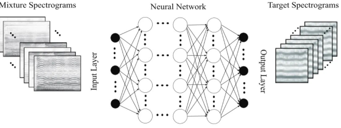
In contrast to the above approaches which require explicit models of the source for processing, methods based on DNNs take advantage of optimization techniques to train source models in a supervised manner [21], [22], [23], i.e. using datasets where both the mix and the isolated sources are available. As depicted in Figure 7, most supervised DNN-based methods take magnitude spectrograms of the audio mix as inputs, optionally also incorporating some further context cues. The targets are set either as the magnitude spectrograms Sj of the desired sources (also shown
in Figure 7), or as their separating masks (either soft masks or binary masks as described in Section III). Regardless of the inputs and targets used, DNN methods work by training the parameters of non-linear functions to minimize the reconstruction error of the chosen outputs (spectrograms or masks) based on the inputs (audio mixes).
The models obtained from a neural network depend on two core aspects. Firstly, the type and quantity of the data used for training is of primary importance. To a large extent, representative training data overcomes the need for explicitly modeling the underlying spectral characteristics
Mixture Spectrograms Neural Network Target Spectrograms
O ut put L aye r Input L aye r
Figure 7: DNN architecture for MSS: Mixture magnitude spectrograms are set as inputs, and source magnitude spectrogram of the desired source Sj are set as the targets.
of the musical sources: they are directly inferred by the network. Secondly, the DNN topology is of great significance, both for the training capabilities of the network and as a means of incorporating prior knowledge in the system.
The earliest DNN-based approaches for MSS consisted of taking a given frame of the spec-trogram, as well as additional context frames as input, and outputting the corresponding frame for each of the targets. These systems mostly consisted of fully-connected networks (FCN). However, given the large size of music spectrograms, the resulting FCNs contained a large number of parameters. This restricted the use of temporal context in such networks to less than one second [22]. Therefore, these networks were typically applied on sliding windows of the mixture spectrogram. To overcome this limitation, both recurrent neural networks (RNNs) and convolutional neural networks were investigated as they offered a principled way to learn dynamic models. RNNs are similar to FCNs, except that they apply their weights recursively over an input sequence, and can process sequential data of arbitrary length. This makes such dynamical models ideally suited for the processing of spectrograms of different tracks with different durations, while still modeling long term temporal dependencies. The most commonly used setting for DNN-based separation today is to fix the number and the nature of the sources to separate beforehand. For example, we may learn a network able to separate drums, vocals and bass from a mixture. However, having MSS systems which can dynamically detect and separate an arbitrary number of sources is an open challenge, and deep clustering [24] methods represent a possible approach to designing such systems.
A limitation of many DNN models is that they often use Mean Squared Error (MSE) as a cost function. While MSE results in a well-behaved stochastic gradient optimization problem, it also poorly correlates with perceived audio quality. This is the reason why the design of more appropriate cost functions is also an active research topic in MSS [23].
Finally, a crucial limitation of current research for DNN-based MSS is the need for large amounts of training data. The largest MSS multi-track public dataset today is MUSDB 2, which comprises 10 h of data 3. However, this is still small compared to existing speech corpora comprising hundreds or thousands of hours. The main difficulty in creating realistic multi-track data sets for MSS, comes from the fact that individual recordings for each instrument in a mixture
2MUSDB: https://doi.org/10.5281/zenodo.1117372
3Refer to the accompanying website for more information about available data sets: https://soundseparation.songquito.
are rarely available. Conversely, if individual recordings of instruments are available, the process of creating a realistic music mixture with them is time-consuming and very costly (as outlined in Section II). As a result, designing DNN architectures for MSS still requires fundamental knowledge about the sources to be separated, their input and output representations, as well as the use of suitable signal processing techniques and post-processing operations to further improve the recovered sources.
V. EVALUATION OFMUSICALSOURCESEPARATIONMODELS
Once an MSS system has been developed, its performance needs to be evaluated. All MSS approaches invariably introduce unwanted artifacts in the separated sources. These artifacts can be caused by mismatches between the models and the sources, musical noise that appears whenever rapid phase or spectral changes are introduced in the estimates (for example, when using binary masking), reconstruction errors in re-synthesis, as well as phase errors in the estimates. Quality evaluation in MSS systems is however non-trivial. As musical signals are intended to be heard by human listeners, it is therefore reasonable that evaluation should be based on subjective listening tests such as the Multiple Stimulus with Hidden Reference and Anchors (MUSHRA) test [25]. However, listening tests are time-consuming and costly, requiring human volunteers to undertake the tests, and need certain expertise to be conducted properly. This has made them an infrequent choice for separation quality evaluation.
In an attempt to reduce the efforts of evaluating MSS systems, objective quality metrics have been proposed in the literature. These include the Blind Source Separation Evaluation (BSS Eval) Toolbox [26], based on non-perceptual energy ratios, and the Perceptual Evaluation methods for Audio Source Separation (PEASS)toolkit [27], which aimed to map results obtained via listening tests to create metrics. However, the validity of these metrics has been questioned in recent years, as the values obtained with them do not seem to correlate with perceptual measures obtained via listening tests [28].
As of today, given the lack of an unified and perceptually valid strategy for MSS quality evaluation, most algorithm development is still conducted using BSS Eval; however, it is highly recommended to conduct a final listening test to verify the validity of separation results. As a final note, the source separation community runs a regular Signal Separation Evaluation Campaign (SiSEC) [29] including musical audio source separation tasks. SiSEC raises the visibility and importance of evaluation, and acts as a focus for discussions on evaluation methodologies.
VI. FUTURERESEARCHDIRECTIONS
Musical Source Separation is a challenging research area with numerous real-world applica-tions. Due to both the nature of the musical sources and the very particular processes used to create music recordings, MSS has many unique features and problems which make it distinct from other types of source separation problems. This is further complicated by the need to achieve separations which sound good in a perceptual sense.
While the quality of MSS has greatly improved in the last decade, several critical challenges remain. Firstly, audible artifacts are still produced by most algorithms. Possible research directions to reduce artifacts include the use of phase retrieval techniques to estimate the phase of the target source, the use of feature representations that better match human perception, allowing models to concentrate on the parts of the sounds that are most relevant for human listeners, and the exploration of MSS systems that model the signal directly in time domain as waveforms.
Many remaining issues in MSS come from the fact that systems are often not flexible enough to deal with the richness of musical data. For example, it is typically assumed that the actual number of musical sources in a given recording is known. However, this assumption can lead to problems when the number of sources changes over the course of the training procedure. Another issue comes with the separation of sources from the same or similar instrument families, such as the separation of multiple singing voices or violin ensembles.
As previously mentioned, a unified, robust and perceptually valid MSS quality evaluation procedure does not yet exist. Even while new alternatives for evaluation have been explored in recent years [30], listening tests remain the only reliable quality evaluation method to date. The design of new MSS quality evaluation procedures that are applicable for a wide range of algorithms and musical content, will require large research efforts including large-scale listening experiments, common datasets, and the availability of a wide range of MSS algorithms for use in development.
Additionally, a better understanding of how DNN-based techniques can be exploited for music separation is still needed. In particular, we need better training schemes to avoid over-fitting, and architectures suitable for music separation. The inclusion of perceptually-based optimization schemes and availability of training data are also current challenges in the field.
Recent developments in the area of DNNs have introduced a paradigm shift in MSS research, with an increasing focus on data-driven models. Nonetheless, previous techniques have achieved considerable success in tackling MSS problems. We believe that combining the insights gained
from previous approaches with data-driven DNN approaches will allow future researchers to overcome current limitations and challenges in musical source separation.
VII. ACKNOWLEDGMENTS
Mark D. Plumbley is partly supported by grants EP/L027119/2 and EP/N014111/1 from the UK Engineering and Physical Sciences Research Council, and European Commission H2020 “AudioCommons” research and innovation grant 688382. A. Liutkus and F. Stöter are partly supported by the research programme “KAMoulox” (ANR-15-CE38-0003-01) funded by ANR, the French State agency for research.
REFERENCES
[1] A. Hyvärinen, J. Karhunen, and E. Oja, Eds., Independent Component Analysis, Wiley and Sons, 2001. [2] A.S. Bregman, Auditory Scene Analysis: The Perceptual Organization of Sound, MIT Press/Bradford Books,
1990.
[3] N.Q.K. Duong, E. Vincent, and R. Gribonval, “Under-determined reverberant audio source separation using a full-rank spatial covariance model,” IEEE Trans. on Audio, Speech, and Language Processing, vol. 18, no. 7, pp. 1830 –1840, 2010.
[4] Z. Rafii and B. Pardo, “REpeating Pattern Extraction Technique (REPET): A simple method for music / voice separation,” IEEE Trans. on Audio, Speech and Language Processing, vol. 21, no. 1, pp. 73–84, 2013. [5] S. Rickard, The DUET blind source separation algorithm, pp. 217–241, Springer Netherlands, Dordrecht, 2007. [6] D. Barry, B. Lawlor, and E. Coyle, “Real-time sound source separation using azimuth discrimination and
resynthesis,” in 117th Audio Engineering Society (AES) Convention, San Francisco, CA, USA, 2004.
[7] D. FitzGerald, A. Liutkus, and R. Badeau, “Projection-based demixing of spatial audio,” IEEE/ACM Trans. on Audio, Speech, and Language Processing, vol. 24, no. 9, pp. 1560–1572, 2016.
[8] A. Ozerov and C. Févotte, “Multichannel nonnegative matrix factorization in convolutive mixtures for audio source separation,” IEEE Trans. on Audio, Speech and Language Processing, vol. 18, no. 3, pp. 550–563, 2010. [9] A. Liutkus, D. Fitzgerald, Z. Rafii, B. Pardo, and L. Daudet, “Kernel additive models for source separation,”
IEEE Trans. on Signal Processing, vol. 62, no. 16, pp. 4298–4310, 2014.
[10] D. FitzGerald, “Harmonic/percusssive separation using median filtering,” in Proceedings of the 13th International Conference on Digital Audio Effects (DAFx), Graz, Austria, 2010.
[11] D. D. Lee and H. S. Seung, “Algorithms for non-negative matrix factorization,” in Advances in Neural Information Processing Systems (NIPS). Apr. 2001, vol. 13, pp. 556–562, The MIT Press.
[12] T. Virtanen, “Monaural sound source separation by nonnegative matrix factorization with temporal continuity and sparseness criteria,” IEEE Trans. on Audio, Speech, and Language Processing, vol. 15, no. 3, pp. 1066–1074, 2007.
[13] S. Ewert, B. Pardo, M. Mueller, and M. D. Plumbley, “Score-informed source separation for musical audio recordings: An overview,” IEEE Signal Processing Magazine, vol. 31, no. 3, pp. 116–124, 2014.
[14] P. Smaragdis, C. Fevotte, G. J. Mysore, N. Mohammadiha, and M. Hoffman, “Static and dynamic source separation using nonnegative factorizations: A unified view,” IEEE Signal Processing Magazine, vol. 31, no. 3, pp. 66–75, 2014.
[15] J. L. Durrieu, G. Richard, B. David, and C. Fevotte, “Source/filter model for unsupervised main melody extraction from polyphonic audio signals,” IEEE Trans. on Audio, Speech, and Language Processing, vol. 18, no. 3, pp. 564–575, 2010.
[16] P.-S. Huang, S. D. Chen, P. Smaragdis, and M. Hasegawa-Johnson, “Singing-voice separation from monaural recordings using robust principal component analysis,” in IEEE International Conference on Acoustics, Speech and Signal Processing (ICASSP), Kyoto, Japan, Mar. 2012, pp. 57–60.
[17] T.-S. Chan, T.-C. Yeh, Z.-C. Fan, H.-W. Chen, L. Su, Y.-H. Yang, and R. Jang, “Vocal activity informed singing voice separation with the ikala dataset,” in IEEE International Conference on Acoustics, Speech and Signal Processing (ICASSP), Brisbane, Australia, 2015, pp. 718–722.
[18] X. Serra, Musical Sound Modeling with Sinusoids plus Noise, pp. 91–122, Studies on New Music Research. Swets & Zeitlinger, 1997.
[19] T. Virtanen and A. Klapuri, “Separation of harmonic sound sources using sinusoidal modeling,” in IEEE International Conference on Acoustics, Speech, and Signal Processing. Proceedings (ICASSP), Budapest, Hungary, 2000, pp. II765–II768.
[20] E. Cano, M. Plumbley, and C. Dittmar, “Phase-based harmonic/percussive separation,” in 15th Annual Conference of the International Speech Communication Association. Interspeech, Singapore, 2014.
[21] P. S. Huang, M. Kim, M. Hasegawa-Johnson, and P. Smaragdis, “Joint optimization of masks and deep recurrent neural networks for monaural source separation,” IEEE/ACM Trans. on Audio, Speech, and Language Processing, vol. 23, no. 12, pp. 2136–2147, 2015.
[22] S. Uhlich, F. Giron, and Y. Mitsufuji, “Deep neural network based instrument extraction from music,” in IEEE International Conference on Acoustics, Speech and Signal Processing (ICASSP), Brisbane, Australia, 2015, pp. 2135–2139.
[23] A. A. Nugraha, A. Liutkus, and E. Vincent, “Multichannel audio source separation with deep neural networks,” IEEE/ACM Trans. on Audio, Speech, and Language Processing, vol. 24, no. 9, pp. 1652–1664, 2016.
[24] J.R. Hershey, Z. Chen, J. Le Roux, and S. Watanabe, “Deep clustering: Discriminative embeddings for segmentation and separation,” in IEEE International Conference on Acoustics, Speech and Signal Processing (ICASSP), Shanghai, China, 2016, pp. 31–35.
[25] ITU-R, “Recommendation BS.1534-3: Method for the subjective assessment of indermediate quality levels of coding systems,” 10/2015.
[26] E. Vincent, R. Gribonval, and C. Fevotte, “Performance measurement in blind audio source separation,” IEEE Trans. on Audio Speech Language Processing, vol. 14, no. 4, pp. 1462–1469, 2006.
[27] V. Emiya, E. Vincent, N. Harlander, and V. Hohmann, “Subjective and Objective Quality Assessment of Audio Source Separation,” IEEE Trans. on Audio, Speech, and Language Processing, vol. 19, no. 7, pp. 2046–2057, 2011.
[28] E. Cano, D. FitzGerald, and K. Brandenburg, “Evaluation of quality of sound source separation algorithms: Human perception vs quantitative metrics,” in European Signal Processing Conference (EUSIPCO), Budapest, Hungary, 2016, pp. 1758–1762.
separation evaluation campaign,” in International Conference on Latent Variable Analysis and Signal Separation. Springer, 2017, pp. 323–332.
[30] D. Ward, H. Wierstorf, R.D. Mason, E. M. Grais, and M.D. Plumbley, “BSS Eval or PEASS? Predicting the perception of singing-voice separation,” in IEEE International Conference on Acoustics, Speech and Signal Processing (ICASSP), Calgary, Canada, 2018.
Estefanía Cano, holds degrees in Electronic Engineering (B.Sc), Music-Saxophone Performance (B.A), Music Engineering (M.Sc), and Media Technology (PhD). In 2009, she joined the Semantic Music Tech-nologies group at the Fraunhofer Institute for Digital Media Technology IDMT as a research scientist. In 2018, she joined the Music Cognition Group at the Agency for Science, Technology and Research A*STAR in Singapore. Her research interests include sound source separation, analysis and modeling of musical instrument sounds and the use of music information retrieval techniques in musicological analysis.
Derry FitzGerald has degrees in Chemical Engineering (B.Eng), Music Technology (M.A) and Digital Signal Processing (PhD). He has worked as a Research Fellow at both Cork and Dublin Institutes of Technology and is currently CTO at AudioSourceRE, a start-up developing sound source separation technologies. His research interests are in the areas of sound source separation, and tensor factorizations.
Antoine Liutkus received the State Engineering degree from Telecom ParisTech, France, in 2005, and the M.Sc. degree in acoustics, computer science and signal processing applied to music (ATIAM) from the Université Pierre et Marie Curie (Paris VI), Paris, in 2005. He worked as a research engineer on source separation at Audionamix from 2007 to 2010 and obtained his PhD in electrical engineering at Telecom ParisTech in 2012. He is currently researcher at Inria Nancy Grand Est in the speech processing team. His research interests include audio source separation and machine learning.
Prof. Mark D. Plumbley was awarded the PhD degree in neural networks from Cambridge University Engineering Department in 1991, then becoming a Lecturer at King’s College London. He moved to Queen Mary University of London in 2002, later becoming Professor of Machine Learning and Signal Processing, and Director of the Centre for Digital Music. He then joined the University of Surrey in January 2015 to become Professor of Signal Processing in the Centre for Vision, Speech and Signal Processing (CVSSP). His research concerns the analysis and processing of audio and music, using a wide range of signal processing techniques, including independent component analysis (ICA) and sparse representations.
Fabian-Robert Stöter received the diploma degree in electrical engineering in 2012 from the Leibniz Universität Hannover and worked towards his Ph.D. degree in audio signal processing in the research group of B. Edler at the International Audio Laboratories Erlangen, Germany. He is currently a researcher at Inria/LIRMM Montpellier, France. His research interests include supervised and unsupervised methods for audio source separation and signal analysis of highly overlapped sources.