Collaborating

The MIT Faculty has made this article openly available.

Please share

how this access benefits you. Your story matters.

Citation

Bonatti, Alessandro, and Johannes Hörner. 2011. "Collaborating."

American Economic Review, 101(2): 632–63.

As Published

http://dx.doi.org/10.1257/aer.101.2.632

Publisher

American Economic Association

Version

Final published version

Citable link

http://hdl.handle.net/1721.1/65916

Terms of Use

Article is made available in accordance with the publisher's

policy and may be subject to US copyright law. Please refer to the

publisher's site for terms of use.

=10.1257/aer.101.2.632

632

Teams and partnerships are playing an increasingly important role in economic activity, at the levels of individual agents and firms alike. In research, for instance, we observe an apparent shift from the individual-based model to a teamwork model, as documented by Stefan Wuchty, Benjamin F. Jones, and Brian Uzzi (2007). In busi-ness, firms are using collaborative methods of decision making more and more, so the responsibility for managing a project is shared by the participants (see Michael Hergert and Deigan Morris 1988_{). Yet despite the popularity of joint ventures, firms} experience difficulties in running them.

The success of such ventures relies on mutual trust, such that each member of the team believes that every other member will pull his weight. However, it is often dif-ficult to distinguish earnest, but unlucky, effort from free-riding because the duration and outcome of the project are uncertain. This difficulty has practical consequences in cases of persistent lack of success. In such cases, agents may grow suspicious that other team members are not pulling their weight in the common enterprise and scale back their own involvement in response, which will result in disruptions and, in some cases, the ultimate dissolution of the team. There is a large literature in management that documents the difficulties involved in running joint ventures and the risks of shirking that are associated with them (see, for instance, Anoop Madhok 1995; Yadong Luo 2002_{). Yaping Gong et al. (2007) show how cooperation in} inter-national joint ventures decreases as the number of partners increases, and relate their finding to the increased room for opportunistic behavior that arises as the venture becomes larger and more complex.

Collaborating

By Alessandro Bonatti and Johannes Hörner*

This paper examines moral hazard in teams over time. Agents are collectively engaged in a project whose duration and outcome are uncertain, and their individual efforts are unobserved. Free-riding leads not only to a reduction in effort, but also to procrastination. Collaboration among agents dwindles over time, but does not cease as long as the project has not succeeded. In addition, the delay until the project succeeds, if it ever does, increases with the number of agents. We show why deadlines, but not necessarily better monitor-ing, help to mitigate moral hazard. (JEL D81, D82, D83)

* Bonatti: MIT Sloan School of Management, 50 Memorial Drive, Cambridge MA 02142 (e-mail: bonatti@mit. edu); Hörner: Department of Economics, Yale University, 30 Hillhouse Avenue, New Haven, CT 06520 (e-mail: johannes.horner@yale.edu). We would like to thank Dirk Bergemann, Martin Cripps, Glenn Ellison, Meg Meyer, David Miller, Motty Perry, Sven Rady, Larry Samuelson, Roland Strausz, and Xavier Vives for useful discussions, and Nicolas Klein for excellent comments. We thank Glenn Ellison for providing us with the data that is used in the working paper. Finally, we thank three anonymous referees, whose suggestions have led to numerous improve-ments to the paper. In particular, their suggestions led to Sections I, VE, and a large part of IVA. Hörner gratefully acknowledges support from NSF grant 0920985.

This paper provides a model of how teams work toward their goals under condi-tions of uncertainty regarding the duration and outcome of the project, and exam-ines possible remedies. Our model may be applied both intrafirm, for example, to research teams, and interfirm, for example, to R&D joint ventures and alliances. The benefits of collaborative research are widely recognized, and R&D joint ventures are encouraged under both US and EU competition law and funding programs.1 Nevertheless, any firm that considers investing resources in such projects faces all the obstacles that are associated with contributing to a public good.

With very few exceptions, previous work on public goods deals with situations that are either static or involve complete information. This work has provided invalu-able insights into the quantitative underprovision of the public good. In contrast, we account explicitly for uncertainty and learning, and therefore concentrate our atten-tion on the dynamics of this provision.2

The key features of our model are as follows: _{(i) Benefits are public, costs are}

pri-vate: the value from completing the project is common to all agents. All it takes to complete the project is one breakthrough, but making a breakthrough requires costly effort. (ii) Success is uncertain: some projects will fail, no matter how much effort is put into them, due to the nature of the project, though this will not, of course, be known at the start.3 As for those projects that can succeed, the probability of making a breakthrough increases as the combined effort of the agents increases. Achieving a breakthrough is the only way to ascertain whether a project is one that must fail or can succeed. _{(iii) Effort is hidden: the choice of effort exerted by an agent is} unobserved by the other agents. As long as there is no breakthrough, agents will not have any hard evidence as to whether the project can succeed; they simply become (weakly) more pessimistic about the prospects of the project as time goes on. This captures the idea that output is observable, but effort is not. We shall contrast our findings with the case in which effort is observable. At the end of the paper, we also discuss the intermediate case, in which the project involves several observable steps.

Our main findings are the following:

• Agents procrastinate: as is to be expected, agents slack off, i.e., there is under-provision of effort overall. Agents exert too little effort, and exert it too late. In the hope that the effort of others will suffice, they work less than they should early on, postponing their effort to a later time. Nevertheless, due to growing pessimism, the effort expended dwindles over time, but the plug is never pulled on the project. Although the overall effort expended is independent of the size 1 _{More specifically, R&D joint ventures enjoy a block exemption from the application of Article 81(3) of the EU}

Treaty, and receive similar protection in the United States under the National Cooperative Research and Production Act and the Standards Development Organization Advancement Act. Further, cooperation on transnational research projects was awarded 64 percent of the nonnuclear, €51 billion budget under the 2007–2013 7th Framework Programs of the European Union for R&D.

2 _{The management literature also stresses the importance of learning in alliances. For example, Yves L. Doz and}

Gary Hamel (1998) claim that to sustain successful cooperation, partners typically need to learn in five key areas: the environment in which the alliance will operate, the tasks to be performed, the process of collaboration, the partners’ skills, and their intended and emerging goals.

3 _{This is typically the case in pharmaceutical research. Doz and Hamel (1998) report that the pharmaceutical}

giant Merck assembled a complex network of research institutes, universities, and biotechnology companies to develop AIDS vaccines and cures in the early 1990s. Given the serendipitous nature of pharmaceutical innovations, there was no way of knowing which, if any, part of this web of R&D alliances would be productive.

of the team, the more agents are involved in the project, the later the project gets completed on average, if ever.

• deadlines are beneficial: if agents have enough resolve to fix their own dead-line, it is optimal to do so. This is the case despite the fact that agents pace themselves so that the project is still worthwhile when the deadline is hit and the project is abandoned. If agents could renegotiate at this time, they would. However, even though agents pace themselves too slowly, the deadline gives them an incentive to exert effort once it looms closely enough. The deadline is desirable, because the reduction in wasteful delay more than offsets the value that is forfeited if the deadline is reached. In this sense, delay is more costly than the underprovision of effort.

• Better monitoring need not reduce delay: when effort is observed, there are multiple equilibria. Depending on the equilibrium, the delay might be greater or smaller than under nonobservability. In the unique symmetric Markov equilib-rium, the delay is greater. This is because individual efforts are strategic substi-tutes. The prospects of the team improve if it is found that an agent has slacked off, because this mitigates the growing pessimism in the team. Therefore, an observable reduction in current effort encourages later effort by other members, and this depresses equilibrium effort. Hence, better monitoring need not alle-viate moral hazard. Nevertheless, there are also non-Markovian, grim-trigger equilibria for which the delay is smaller.

We finally discuss how our results can be generalized in several dimensions. We discuss more general mechanisms than deadlines. In particular, we consider the opti-mal dynamic (budget-balanced) compensation scheme, as well as the profit-maxi-mizing wage scheme for a principal who owns the project’s returns. One rationale that underlies the formation of partnerships is the possible synergies that may arise between agents. We consider two types of synergy: _{(i) agents might be identical,} but their combined efforts might be more productive than the sum of their isolated efforts, and _{(ii) agents might have different skills, and depending on the problem} at hand, one or the other might be more likely to succeed.4 We also examine how private information regarding the agent’s productivity and learning-by-doing affect our results. Finally, we remark on the case in which the project involves completing multiple tasks.

This paper is related to several strands of literature. First, our model can be viewed as a model of experimentation. There is a growing literature in economics on experimentation in teams. For instance, Patrick Bolton and Christopher Harris (1999), Godfrey Keller, Sven Rady, and Martin Cripps (2005), and Nicolas Klein and Rady (2008) study a two-armed bandit problem in which different agents may choose different arms. While free-riding plays an important role in these studies as well, effort is always observable. Dinah Rosenberg, Eilan Solan, and Nicolas Vieille (2007), Hugo Hopenhayn and Francesco Squintani (2004), and Pauli Murto and 4 _{This kind of synergy typically facilitates successful collaborations. Doz and Hamel (1998) report the case of}

the Japanese Very Large Scale Integration (VLSI) research cooperative. The VLSI project involved five semicon-ductor manufacturers: Fujitsu, Hitachi, Mitsubishi Electric, NEC, and Toshiba. Interteam cooperation was facili-tated by the choice of overlapping research areas: several teams worked on the same types of topic, but in slightly differentiated ways, thereby providing for original contributions from each team.

Juuso Välimäki (2008) consider the case in which the outcome of each agent’s action is unobservable, while their actions are observable. This is precisely the opposite of what is assumed in this paper; here, actions are not observed, but outcomes are. Dirk Bergemann and Ulrich Hege _{(2005) study a principal-agent} relationship with an information structure similar to the one considered here. All these models provide valuable insights into how much total experimentation is socially desirable, and how much can be expected in equilibrium. As will become clear, these questions admit trivial answers in our model, which is therefore not well suited to address them.

Robin Mason and Välimäki _{(2008) consider a dynamic moral hazard problem} in which effort by a single agent is unobservable. Although there is no learning, the optimal wage declines over time, to provide incentives for effort. Their model shares a number of features with ours. In particular, the strategic substitutability between current and later efforts plays an important role in both models, so that, in both cases, deadlines have beneficial effects. See also Flavio Toxvaerd (2007) on deadlines, and Tracy R. Lewis and Marco Ottaviani _{(2008) on similar effects in the} optimal provision of incentives in sequential search.

Second, our model ties into the literature on free-riding in groups, starting with Mancur Olson (1965) and Armen A. Alchian and Harold Demsetz (1972), and fur-ther studied in Bengt Holmström _{(1982), Patrick Legros and Steven A. Matthews} (1993), and Eyal Winter (2004). In a sequential setting, Roland Strausz (1999) describes an optimal sharing rule. Our model ties in with this literature in that it covers the process by which free-riding occurs over time in teams that are working on a project whose duration and outcome is uncertain; i.e., it is a dynamic version of moral hazard in teams with uncertain output. A static version was introduced by Steven R. Williams and Roy Radner _{(1995) and also studied by Ching-To Ma, John} Moore, and Stephen Turnbull (1988). The inefficiency of equilibria of repeated part-nership games with imperfect monitoring was first demonstrated by Radner, Roger Myerson, and Eric Maskin (1986).

Third, our paper is related to the literature on dynamic contributions to public goods. Games with observable contributions are examined in Anat R. Admati and Motty Perry _{(1991), Olivier Compte and Philippe Jehiel (2004), Chaim Fershtman} and Shmuel Nitzan (1991), Ben Lockwood and Jonathan P. Thomas (2002), and Leslie M. Marx and Matthews _{(2000). Fershtman and Nitzan (1991) compare} open- and closed-loop equilibria in a setup with complete information and find that observability exacerbates free-riding. In Parimal Kanti Bag and Santanu Roy (2008), Christopher Bliss and Barry Nalebuff (1984), and Mark Gradstein (1992), agents have independently drawn and privately known values for the public good. This type of private information is briefly discussed in the conclusion. Applications to partnerships include Jonathan Levin and Steven Tadelis _{(2005) and Barton H.} Hamilton, Jack A. Nickerson, and Hideo Owan (2003). Also related is the literature in management on alliances, including, for instance, Doz _{(1996), Ranjay Gulati} (1995), and Gulati and Harbir Singh (1998).

There is a vast literature on free-riding, also known as social loafing, in social psychology. See, for instance, Bibb Latané, Kipling Williams, and Stephen Harkins (1979), or Steven J. Karau and Williams (1993). Levi (2007) provides a survey of group dynamics and team theory. The stage theory, developed by Bruce W. Tuckman

and Mary Ann C. Jensen (1977) and the theory by Joseph E. McGrath (1991) are two of the better-known theories regarding the development of project teams: the patterning of change and continuity in team structure and behavior over time.

I.  A Simple Example

Consider the following two-period game. Agent i = 1, 2 may exert effort in two periods, t_{= 1, 2, in order to achieve a breakthrough. Whether a breakthrough is} possible depends on the quality of the project. If the project is good, the probability of a breakthrough in period t _{(assuming that there was no breakthrough before) is} given by the sum of the effort levels u i,t that the two agents choose in that period. However, the project might be bad, in which case a breakthrough is impossible. Agents share a common prior belief _ p  < 1 that the project is good.

The project ends if a breakthrough occurs. A breakthrough is worth a payoff of one to both agents, independently of who is actually responsible for this break-through. Effort, on the other hand, entails a private cost given by c_{( u  i,t) in each} period. Payoffs from the second period are discounted at a common factor δ ≤ 1.

Agents do not observe their partner’s effort choice. All they observe is whether a breakthrough occurs. Therefore, if there is no breakthrough at the end of the first period, agents update their belief about the quality of the project based only on their own effort choice, and their expectation about the other agent’s effort choice. Thus, if an agent chooses an effort level u_i,t in each period, and expects his opponent to exert effort  u  _−i,t , his expected payoff is given by

(1)    _ p ⋅ ( u i,1  +      u  _−i,1)  −  c( u i,1)

  8

First period payoff

  +  δ

(

1 −  _ p ⋅ ( u i,1 +     u  _−i,1)

) [

ρ( u i,1 ,  u  _−i,1) ⋅ ( u i,2 +     u  _−i,2) − c( u i,2)

] 

,

  8

Second period payoff

where _{ρ( u i,1} ,  u _{−i,1) is his posterior belief that the project is good. To understand}

(1), note that the probability of a breakthrough in the first period is the product of the prior belief assigned to the project being good ₍_ p _{), and the sum of effort levels}

exerted ( u i,1 +     u  _−i,1). The payoff of such a breakthrough is one. The cost of effort in the first period, c_{( u i,1), is paid in any event. If a breakthrough does not occur, agent i} updates his belief to ρ( u i,1 ,  u  _−i,1), and the structure of the payoff in the second period is as in the first period.

By Bayes’s rule, the posterior belief of agent i is given by (2)  ρ( u i,1 ,  u  _−i,1)  =     _ 

p ⋅(1 −  u i,1 −     u  _−i,1)   

__ _{1 −  _ p ⋅( u}  i,1 +     u  _−i,1)    ≤   _ 

p .

Note that this is based on agent i’s expectation of agent _{− i’s effort choice. That is,} agents’ beliefs are private, and they coincide only on the equilibrium path. If, for

instance, agent i decides to exert more effort than he is expected to by agent − i, yet no breakthrough occurs, agent i will become more pessimistic than agent _− i, unbe-knownst to him. Off path, beliefs are no longer common knowledge.

In a perfect Bayesian equilibrium, agent i’s effort levels _( u i,1 , u_{i,2) are optimal} given (    u  _−i,1 ,  u  _−i,2), and expectations are correct:  u  _−i,t =  u _−i,t . Letting V i denote the agent’s payoff, it must be that

    ∂ _ V i ∂ u i,1

  =   _ p  − c′( u i,1)  −  δ  _ p ⋅ 

(

 u i,2  +      u  _−i,2  −  c( u i,2)

)

  =  0, and

    ∂ _ V i

∂ u i,2

∝  ρ( u i,1 ,  u  _−i,1)  −  c′( u i,2)  =  0,

so that, in particular, c_{′( u i,2) < 1. It follows that (i) the two agents’ first-period effort} choices are neither strategic complements nor substitutes, but (ii) an agent’s effort choices across periods are strategic substitutes, as are _{(iii) an agent’s current effort} choice and the other agent’s future effort choices.

It is evident from _{(ii) that the option to delay reduces effort in the first period.} Comparing the one- and two-period models is equivalent to comparing the first-period effort choice for u_{i,2 =     u  i,2 = 0 on the one hand, and a higher value on the} other. This is what we refer to as procrastination: some of the work that would other-wise be carried out by some date gets postponed when agents get further opportuni-ties to work afterward.5 In our example, imposing a deadline of one period heightens incentives in the initial period.

Further, it is also clear from (iii) that observability of the first period’s action will lead to a decline in effort provision. With observability, a small decrease in the first-period effort level increases the other agent’s effort tomorrow. Therefore, relative to the case in which effort choices are unobservable, each agent has an incentive to lower his first-period effort level in order to induce his partner to work harder in the second period, when his choice is observable.

As we shall see, these findings carry through with longer horizons: deadlines are desirable, while observability, or better monitoring, is not. However, this two-period model is ill-suited to describe the dynamics of effort over time when there is no last period. To address this and related issues, it is best to consider a baseline model in which the horizon is infinite. This model is described next.

II.  The Setup

There are n agents engaged in a common project. The project has a probability

_ p _{< 1 of being a good project, and this is commonly known by the agents. It is a}

bad project otherwise.

Agents continuously choose at which level to exert effort over the infinite horizon ℝ  + . Effort is costly, and the instantaneous cost to agent i = 1, … , n of exerting effort

u i ∈  ℝ  ₊  is c i( u i), for some function c i(⋅) that is differentiable and strictly increasing. In most of the paper, we assume that c_{i( u i) =  c i ⋅  u i}, for some constant c_{i > 0, and} that the choice is restricted to the unit interval, i.e., u i ∈ [0, 1]. The effort choice is, and remains, unobserved.

Effort is necessary for a breakthrough to occur. More precisely, a breakthrough occurs with instantaneous probability equal to f _( u 1 ,_{… ,  u n), if the project is good,} and to zero if the project is bad. That is, if agents were to exert a constant effort u i over some interval of time, then the delay until they found out that the project is successful would be distributed exponentially over that time interval with parameter

f_( u 1 , … , _{u n). The function f is differentiable and strictly increasing in each of its} arguments. In the baseline model, we assume that f is additively separable and linear in effort choices, so that f _( u 1 , … , _{u n) =  ∑   i=1,…,n}     λ i u i , for some λ i > 0, i = 1, … , n.

The game ends if a breakthrough occurs. Let τ ∈  ℝ  ₊  ∪ {+ ∞} denote the ran-dom time at which the breakthrough occurs _{(τ = + ∞ if it never does). We interpret} such a breakthrough as the successful completion of the project. A successful proj-ect is worth a net present value of one to each of the agents.6 As long as no break-through occurs, agents reap no benefits from the project. Agents are impatient, and discount future benefits and costs at a common discount rate r.

If agents exert effort ( u 1 , … ,  u n), and a breakthrough arrives at time t < ∞, the average discounted payoff to agent i is thus

r

(

e −rt  −   

∫ 

0   t

     e −rs _c

i ( u i,s) ds

)

,

while if a breakthrough never arrives (t = ∞), his payoff is simply −  r

∫

0∞       e −rs c i( u i,s) ds. The agent’s objective is to choose his effort so as to maximize his expected payoff.

To be more precise, a _{(pure) strategy for agent i is a measurable function} u i :  ℝ  ₊  → [0, 1], with the interpretation that u i,t is the instantaneous effort exerted by agent i at time t, conditional on no breakthrough having occurred. Given a strat-egy profile u := ( u 1 , … ,  u n), it follows from Bayes’s rule that the belief held in com-mon by the agents that the project is good _{(hereafter, the common belief), p, is given} by the solution to the familiar differential equation

˙

p  t  =  −  p t(1 −  p t) f ( u t),

with p 0 =  _ p .7 Given that the probability that the project is good at time t is p t , and that the instantaneous probability of a breakthrough conditional on this event is

f ( u t), the instantaneous probability assigned by the agent to a breakthrough occurring 6 _{We discuss this assumption further in Section IIIB.}

7 _{To see this, note that, given p}

t, the belief at time t + dt is

pt  +dt  =      p t e  −f ( u t)dt

__ ₁  

 −  p t +  p t e −f ( u t )dt

,

is p _t f ( u _t). It follows that the expected instantaneous reward to agent i at time t

is given by p_t f ( u t) −  c i ( u i,t). Given that the probability that a breakthrough has not occurred by time t is given by exp{− 

∫

₀t       p _s f ( u _s) ds}, it follows that the average

(expected) payoff that agent i seeks to maximize is given by

r

∫ 

0   ∞

  

(

   p t f ( u t)  −   c i( u i,t)

) 

e − ∫0  

t_(  p

s f ( u s)+r) ds _dt.

Given that there is a positive probability that the game lasts forever, and that agent

i’s information set at any time t is trivial, strategies that are part of a Nash equilib-rium are also sequentially rational on the equilibequilib-rium path; hence, our objective is to identify the symmetric Nash equilibria of this game. _{(We shall nevertheless briefly} describe off-the-equilibrium-path behavior as well.)

III.  The Benchmark Model

We begin the analysis with the special case in which agents are symmetric, and both the instantaneous probability and the cost functions are linear in effort:

f ( u 1 , … ,  u n)  =   

∑ 

i=1  

n

     λ i u i,   c i( u i)  =   c i u i ,   u i ∈ [0, 1],   λ i  =  λ,  c i  =  c, for all i.

Equivalently, we may define the normalized cost α := c/λ, and redefine u i , so that each agent chooses the control variable u_{i :  ℝ  +  → [0, λ] so as to maximize}

(3) V_i(_ p _{)  :=  r}

∫ 

0   ∞      

(

 p t

∑ 

i     

      u i,t  −  α u i,t

)

e − ∫0  

t_(  p s ∑ i          u i,s+r) ds _dt, subject to ˙ p _{t  =  −  p t(1 −  p t)}

∑ 

i            u i,t, p 0  =   _ p .

Observe that the parameter α is the Marshallian threshold: it is equal to the belief at which a myopic agent would stop working, because at this point the instantaneous marginal revenue from effort, p t, equals the marginal cost, α.

A. The Team problem

If agents behaved cooperatively, they would choose efforts so as to maximize the sum of their individual payoffs, that is,

W( _ p )  :=   

∑ 

i=1   n      V i( _ p )  =  r

∫ 

0   ∞      (n p t − α)  u t e − ∫0   t_(  p s u s+r) ds _dt,

where, with some abuse of notation, u t :=   ∑ _i        u i,t ∈ [0, nλ]. The integrand being positive as long as p_{t  ≥  α/n, it is clear that it is optimal to set u t} equal to n_{λ as long} as p t ≥ α/n, and to zero otherwise. The belief p t is then given by

p_{t  =}__  _ p 

 

_ p  + (1 −  _ p ) e nλt ,

as long as the right-hand side exceeds _{α/n. In short, the team solution specifies that} each agent sets his effort as follows:

u_{i,t  =  λ if t  ≤   T n  :=  (nλ )}−1 ln _ _ p (1 − α/n) 

(1 −  _ p _)α/n , and u i,t  =  0 for t  >   T n. Not surprisingly, the resulting payoff is decreasing in the discount rate r and the normalized cost α, and increasing in the prior _ p , the upper bound λ, and the number of agents n.

Observe that the instantaneous marginal benefit from effort to an agent is equal to p_t, which decreases over time, while the marginal cost is constant and equal to α. Therefore, it will not be possible to provide incentives for selfish agents to exert effort beyond the Marshallian threshold. The wedge between this threshold and the efficient one, α/n, captures the well-known free-riding effect in teams, which is described eloquently by Alchian and Demsetz _{(1972), and has since been studied} extensively. In a noncooperative equilibrium, the amount of effort is too low.8 Here, instead, our focus is on how free-riding affects when effort is exerted.

B. The noncooperative Solution

As mentioned above, once the common belief drops below the Marshallian threshold, agents do not provide any effort. Therefore, if _ p  ≤ α, there is a unique

equilibrium, in which no agent ever works, and we might as well assume throughout that _ p  > α. Further, we assume throughout this section that agents are sufficiently

patient. More precisely, the discount rate satisfies (4)    λ _ r   ≥   α −1 −   _ p    −1  >  0.

This assumption ensures that the upper bound on the effort level does not affect the analysis.9 The proof of the main result of this section relies on Pontryagin’s princi-ple, but the gist of it is perhaps best understood by the following heuristic argument from dynamic programming.

What is the trade-off between exerting effort at some instant and exerting it at the next? Fix some date t, and assume that players have followed the equilibrium strate-gies up to that date. Fix also some small dt_{> 0, and consider the gain or loss from}

8 _{There is neither an “encouragement effect” in our setup, unlike in some papers on experimentation (see, for}

instance, Bolton and Harris 1999), nor any effect of patience on the threshold. This is because a breakthrough yields a unique lump sum to all agents, rather than conditionally independent sequences of lump sum payoffs.

shifting some small effort ε from the time interval [t, t + dt] (“today”) to the time interval _{[t + dt, t + 2dt] (“tomorrow”). Write u i}, p for u_i,t, p_t, and u_{i  ′  , p′ for u i,t+dt} ,

p t+dt , and let Vi,t   , or V i , denote the unnormalized continuation payoff of agent i at time t. The payoff V_i,t must satisfy the recursion

V_{i,t    =}

(

_{p( u i +  u −i) − α u i}

) 

dt_{+  (1 − rdt)}

(

1_{− p( u i +  u −i) dt}

) 

V_i,t  +dt . Because we are interested in the trade-off between effort today and tomorrow, we apply the same expansion to Vi,t  _+dt , to obtain

(5) V  i,t  =   

( 

p ( u i +  u _−i) − α u i) dt

  +  (1 − r dt)

(

1 − p( u i +  u _−i) dt

)

  × 

[

(

 p′( u  i  ′  +  u  _−i′   ) − α u     i  ′    

) 

dt + (1 − r dt)

(

1 − p′( u  i  ′  +  u  _−i′   ) dt  

)

 V i,t_{+2 dt}

]

, where p_{′  = p − p(1 − p)( u}i +  u _−i) dt.10 Consider, then, decreasing u i by ε and increasing u_{i  ′  by that amount. Note that, conditional on reaching t + 2 dt without a} breakthrough, the resulting belief is unchanged, and, therefore, so is the continua-tion payoff. That is, V_{i,t  +2dt} is independent of _ε.

Therefore, to the second order,

d V i,t/dε  _ _dt   =  − ((p − α) − p V i,t

)

  +  ( p − α) − p V i,t  =  0. 5 5 dV i,t/du i _ dt ⋅    du i _ _{dε      _}d V i,t/d u  i′     dt ⋅    d u  i′     _ _dε 

To interpret this, note that increased effort affects the payoff in three ways: it increases the probability of a breakthrough, yielding a payoff of one, at a rate p_t ; it causes the loss of the continuation value V i,t at the same rate; lastly, it increases cost, at a rate _α.

The upshot of this result is that the trade-off between effort today and tomorrow can only be understood by considering an expansion to the third order. Here we must recall that the probability of a breakthrough given effort level u is, to the third order, pudt_{− ( pu )}2_{(dt )}2_{/2 (see footnote 10); similarly, the continuation payoff is} discounted by a factor e −rdt ≈ 1 − r dt +  r  2_{(dt )}2_/2.

Let us first expand terms in _{(5), which gives}

V_{i,t  =  ( pu − α  u i) dt − ( pu )}2 _{(d t)}2_{/2  +  (1 − (r + pu) dt + (r + pu )}2 _{d t} 2_/2)   ×  [( p u′  − α  u  i′ )dt − 

(

(1 − p)u + pu′/2

)

pu′ dt 2

  +  [1 − (r + p u′ ) dt + 

(

(r + pu′   )2_{/2 + p(1 − p)u u′  ) dt} 2

]

_V i,t+2 dt

]

,

10 _{More precisely, for later purposes, e}−p ( u i + u −i) dt_{=  1 − p( u}

where, for this equation and the next, u :=  u i +  u _−i, u′  :=   u  i  ′  +  u  _−i′   . We then obtain,    ignoring the second-order terms that, as shown, cancel out,

d V i,t/dε  _ _{d t}   2     −   _ dV i,t/du i d t  2 ⋅    du i _ _dε   

6

    =   p  2 _{u + p( p u′ (1 −  V}

i) − α u  i  ′  − r V i) − (r + pu)p V i + p(1 − p) u′ (1 −  V i)     +  p(r + p u′ ) V i − p(1 − p)u(1 −  V i) −  p 2 u′  − (r + pu)( p(1 −  V i) − α).

 

8

    _{_}dV i, t/du  i′    

d t  2 ⋅    d u  i  ′  

_ _{d ε} 

Assuming that u i and u _−i are continuous, almost all terms vanish. We are left with

_ d V i,t/d ε 

d t 2   =  αp( u i  +   u −i)  −  r ( p  −  α)  −  α  p u i. This means that postponing effort to tomorrow is unprofitable if and only if (6)  α  p u i  ≥  α   p ( u i  +   u −i)  −  r( p  −  α).

Equation _{(6) admits a simple interpretation. What is the benefit of working a bit} more today, relative to tomorrow? At a rate p (the current belief), working today increases the probability of an immediate breakthrough, in which event the agent will not have to pay the cost of the planned effort tomorrow (α   u i ). This is the left-hand side. What is the cost? If the agent waited until tomorrow before working a bit harder, there is a chance that this extra effort would not have to be carried out. The probability of this event is p _{⋅ ( u i +  u −i), and the cost saved is α per unit of extra} effort. This gives the first term on the right-hand side. Of course, there is also a cost of postponing, given that agents are impatient. This cost is proportional to the mark-up of effort, p − α, and gets subtracted on the right-hand side.

First, observe that, as p _{→ α, the right-hand side of (6) exceeds the left-hand side} if u _−i is bounded away from zero. Effort tends to zero as p tends to α. Similarly, effort must tend to zero as r _→ 0.

Second, assume for the sake of contradiction that agents stop working at some finite time. Then, considering the penultimate instant, it must be that, up to the sec-ond order, p − α  =  p(1 − p)( u i +  u _−i) dt, and so we may divide both sides of (6) by u_{i +  u −i  =  n u i} , yielding

p _{(1  −  p)r dt  ≥    n − 1} _ _{n α p,}

which is impossible, as dt is arbitrarily small. Therefore, not only does effort go to zero as p tends to α, but it does so sufficiently fast that the belief never reaches the

threshold α, and agents keep on working on the project forever, albeit at negligible rates.

It is now easy to guess what the equilibrium value of u i must be. Given that agent

i must be indifferent between exerting effort or not, and also exerting it at different instants, we must have

  α  p u i  =  α   p ( u i  +   u −i)  −  r ( p  −  α), or ui ( p)  =    

r _(α−1 _{− p}−1₎

 

__ _{n −  1} . Hence, the common belief tends to the Marshallian threshold asymptotically, and total effort, as a function of the belief, is actually decreasing in the number of agents. To understand this last result, observe that the equilibrium reflects the logic of mixed strategies. Because efforts are perfect substitutes, the indifference condition of each agent requires that the total effort by all agents but him be a constant that depends on the belief, but not on the number of agents. Thus, each agent’s level of effort must be decreasing in the number of agents. In turn, this implies that the total effort by all agents for a given belief is the sum of a constant function and of a decreasing function of the number of agents. Therefore, it is decreasing in the number of agents.

This simple logic relies on two substitutability assumptions: efforts of different agents are perfect substitutes, and the cost function is linear. Both assumptions will be relaxed later.

We emphasize that, because effort is not observed, players share a common belief only on the equilibrium path. For an arbitrary history, an agent’s best-reply depends both on the public and on his private belief. Using dynamic programming is difficult, because the optimality equation is then a partial differential equation. Pontryagin’s principle, on the other hand, is ideally suited, because the other agents’ strategies can be viewed as fixed, given the absence of feedback.

The next theorem, proved in the Appendix, describes the strategy on the equilib-rium path.11

THEOREM 1: There exists a unique symmetric equilibrium, in which, on the

equi-librium path, the level of effort of any agent is given by (7) u  i,t*      =     r _ _n − 1 α 

−1_− 1

__    

1 +   (_ 1_{_ p}  −  _− α_ p )α   

 e    n _ _n−1 r ( α −1_−1)t , for all t  ≥  0.

If an agent deviated, what would his continuation strategy be? Suppose that this deviation is such that, at time t, the aggregate effort of agent i alone over the interval [0, t] is lower than it would have been on the equilibrium path. This means that agent

i is more optimistic than the other agents, and his private belief exceeds their com-mon belief. Given that agent i would be indifferent between exerting effort or not if he shared the common belief, his optimism leads him to exert maximal effort until 11 _{In the case} _ _{p   =  1 that was ruled out earlier, the game reduces essentially to the static game. The effort level}

the time his private belief catches up with the other agents’ common belief, at which point he will revert to the common, symmetric strategy. If, instead, his realized aggregate effort up to t is greater than in equilibrium, then he is more pessimistic than the other agents, and he will provide no effort until the common belief catches up with his private belief, if ever. This completes the description of the equilib-rium strategy. In Section VA, we characterize asymmetric equilibria of the baseline model, and allow for asymmetries in the players’ characteristics.

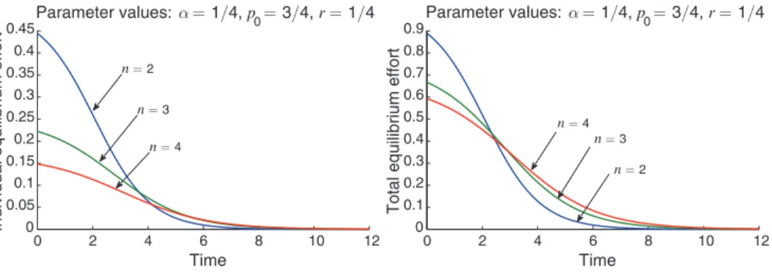
From _{(7), it is immediate to derive the following comparative statics. To avoid} confusion, we refer to total effort at time t as the sum of instantaneous, individual effort levels at that time, and to aggregate effort at t as the sum _{(i.e., the integral) of} total effort over all times up to t.

LEMMA 1: In the symmetric equilibrium:

(i) Individual effort decreases over time and increases _ p .

(ii) Aggregate effort decreases in α and increases in r. It also decreases in, but is

asymptotically independent of, n: the probability of an eventual breakthrough is independent of the number of agents, but the distribution of the time of the breakthrough with more agents first-order stochastically dominates this dis-tribution with fewer agents.

 (iii) The agent’s payoff V i (  _ p ) is increasing in n and _ p , decreasing in α, and

inde-pendent of r.

Total effort is decreasing in n for a given belief p, so that total effort is also decreasing in n for small enough t. However, this implies that the belief decreases more slowly with more agents. Because effort is increasing in the belief, it must then be that total effort is eventually higher in larger teams. Because the asymptotic belief is _{α, independent of n, aggregate effort must be independent of n as well. Ultimately,} then, larger teams must catch up in terms of effort, but this also means that larger teams are slower to succeed.12

In particular, for teams of different sizes, the distributions of the random time τ of a breakthrough, conditional on a breakthrough occurring eventually, are ranked by first-order stochastic dominance. We define the expected cost of delay as 1_− E[ e−r τ_{| τ  <  ∞]. It follows from Lemma 1 that the cost of delay is increasing in}

n. However, it is independent of r, because more impatient agents work harder, but discount the future more. As mentioned above, the agents’ payoffs are also increas-ing in n. This is obvious for one versus two agents, because an agent may always act as if he were by himself, securing the payoff from a single-agent team. It is less obvious that larger, slower teams achieve higher payoffs. Our result shows that, for larger teams, the reduction in individual effort more than offsets the increased cost of delay. Figure 1 and the left panel of Figure 2 illustrate these results.

12 _{As a referee observed, this is reminiscent of the bystander effect, as in the Kitty Genovese case: because more}

agents are involved, each agent optimally scales down his involvement, resulting in an outcome that worsens with the number of agents.

Note that the comparative statics with respect to the number of agents hinge upon our assumption that the project’s returns per agent were independent of n. If, instead, the total value of the project is fixed independently of n, so that each agent’s share decreases linearly in n, aggregate effort decreases with the team’s size, and tedious calculations show that each agent’s payoff decreases as well. See the right panel of Figure 2 for an illustration.

C. A Comparison with the observable Case

We now contrast the previous findings with the corresponding results for the case in which effort is perfectly observable. That is, we assume here that all agents’ efforts are observable, and that agent i’s choice as to how much effort to exert at time t _{(hereafter, his effort choice) may depend on the entire history of effort choices} up to time t. Note that the “cooperative,” or socially optimal, solution is the same whether effort choices are observed or not: delay is costly, so that all work should be carried out as fast as possible; the threshold belief beyond which such work is unprofitable must be, as before, p_{= α/n, which is the point at which marginal} ben-efits of effort to the team are equal to its marginal cost.

0 2 4 6 8 10 12 0 0.05 0.1 0.15 0.2 0.25 0.3 0.35 0.4 0.45 Time

Individual equilibrium effort

Parameter values: α = 1/4, p₀= 3/4, r = 1/4 n = 2 n = 4 n = 3 0 2 4 6 8 10 12 0 0.1 0.2 0.3 0.4 0.5 0.6 0.7 0.8 0.9 Time

Total equilibrium effort

n = 2

n = 3

n = 4

Parameter values: α = 1/4, p₀= 3/4, r = 1/4

Figure 1. Individual and Total Effort

2 4 6 8 10 12 0.1 0.2 0.3 0.4 0.5 0.6 Number of agents

Payoffs, expected cost of delay

Parameter values: α = 1/4, p₀ = 3/4, r = 1/20 Payoffs Cost of delay 2 3 4 5 6 7 8 9 −0.1 0 0.1 0.2 0.3 0.4 0.5 0.6 0.7 0.8 Number of agents

Payoffs, expected cost of delay

Payoffs Cost of delay Parameter values: α = 1/10, p₀ = 9/10, r = 1/20

Figure 2. Payoffs and Cost of Delay

Such a continuous-time game involves well-known nontrivial modeling choices. A standard way to sidestep these choices is to focus on Markov strategies. Here, the obvious state variable is the belief p. Unlike in the unobservable case, this belief is always commonly held among agents, even after histories off the equilibrium path.

A strategy for agent i, then, is a map u i  : [0, 1] → [0, λ] from possible beliefs

p into an effort choice u_{i ( p), such that (i) u i} is left-continuous; and _{(ii) there is a} finite partition of [0, 1] into intervals of strictly positive length on each of which

u_i is Lipschitz-continuous. By standard results, a profile of Markov strategies u_(⋅) uniquely defines a law of motion for the agents’ common belief p, from which the (expected) payoff given any initial belief p can be computed (cf. Ernst L. Presman 1990; Presman and Isaac M. Sonin 1990). A Markov equilibrium is a profile of Markov strategies such that, for each agent i, and each belief p, the function u_i maxi-mizes i’s payoff given initial belief p. See, for instance, Keller, Rady, and Cripps (2005) for details. Following standard steps, agent i’s continuation payoff given p,

V i( p), must satisfy the optimality equation for all p, and dt  >  0. This equation is given by, to the second order,

V_{i( p)   =}   max  _u     

i

{(

( u i  +   u −i)  p t  −   u i α

)

dt  + 

(

1  − 

(

r  +  ( u i  +   u −i) p t

) 

dt

)

V i ( p t+dt)

}

  =  max   _u i

{(

_{( u i +   u −i) p −  u i α) dt  +  (1  −  (r  +  ( u i +  u −i)p) dt)}

  ×   

(

V_{i ( p)  −  ( u i +  u −i) p (1 − p) V  i  ′  ( p) dt)}

}

. Taking limits as dt _{→ 0 yields}

0₌  max  _u    

i

{(

u i +  u −i

)

p −  u i α − 

(

r + ( u i +  u −i)  p

)(

V i ( p)  − ( u i +  u −i)p(1 − p)  V  i  ′  ( p)

}

,

assuming, as will be verified, that V is differentiable. We focus here on a symmetric equilibrium in which the effort choice is interior. Given that the maximand is linear in u_i, its coefficient must be zero. That is, dropping the agent’s subscript,

p_{−  α  −  pV ( p)   −  p (1  −  p) V ′( p)  =  0,}

and since V _{(α)   =  0, the value function is given by}

V _{(p)   =  p  −  α  +  α(1  −  p) ln} _ (1 − p) α 

 (1 − α) p .

Plugging back into the optimality equation, and solving for u :=  u  i , all i, we get

u_{( p)  =}_ r

α(n − 1)   V (p)   =    _ α(n − 1)   r

(

p − α + α(1 − p)ln _ (1 − p) α  (1 − α) p

)

. It is standard to verify that the resulting u is the unique equilibrium strategy pro-file provided that _ p is such that u ≤ λ for all p <  _ p . In particular, this is satis-fied under assumption _{(4) on the discount rate, which we maintain henceforth. In} the model without observability, recall that, in terms of the belief p, effort is given

by u( p) = 

(

r/(n − 1)

)

( α −1 −  p −1). As is clear from these formulas, the eventual

belief is the same whether effort is observed or not, and so aggregate effort over time is the same in both models. However, delay is not.

THEOREM 2: In the symmetric Markov equilibrium with observable effort, the

equilibrium level of effort is strictly lower, for all beliefs, than that in the

unobserv-able case.

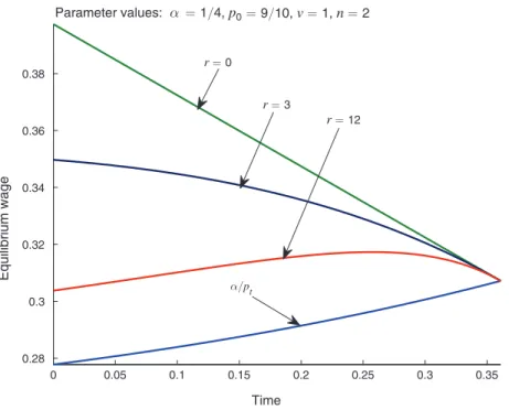
Thus, fixing a belief, the instantaneous equilibrium level of effort is lower when previous choices are observable, and so is welfare. This means that delay is greater under observability. While this may be a little surprising, it is an immediate con-sequence of the fact that effort choices are strategic substitutes. Because effort is increasing in the common belief, and because a reduction in one agent’s effort choice leads to a lower rate of decrease in the common belief, such a reduction leads to a greater level of subsequent effort by other agents. That is, to some extent, the other agents take up the slack. This depresses the incentives to exert effort and leads to lower equilibrium levels. This cannot happen when effort is unobservable, because an agent cannot induce the other agents into “exerting the effort for him.” Figure 3 illustrates this relationship for the case of two players. As can be seen from the right panel, a lower level of effort for every value of the belief p does not imply a lower level of effort for every time t: given that the total effort over the infinite horizon is the same in both models, levels of effort are eventually higher in the observable case.

The individual payoff is independent of the number of agents n_{≥ 2 in the} observable case. This is a familiar rent-dissipation result: when the size of the team increases, agents waste in additional delay what they save in individual cost. This can be seen directly from the formula for the level of effort, in that the total effort of all agents but i is independent of n. It is worth pointing out that this is not true in the unobservable case. This is one example in which the formula that gives the effort as a function of the common belief is misleading in the unobservable case: given p, the total instantaneous effort of all agents but i is independent of n here as well. Yet the

2 4 6 8 10 12 0.54 0.55 0.56 0.57 0.58 0.59 0.6 0.61 0.62 0.63 0.64 Number of agents Equilibrium payoffs Unobservable Observable 0 2 4 6 8 10 12 14 16 18 20 0 0.1 0.2 0.3 0.4 0.5 0.6 0.7 0.8 0.9 1 Time

Individual equilibrium effort

Unobservable Observable Team solution

Parameter values: α = 1/4, p₀ = 3/4, r = 1/20 Parameter values: α = 1/4, p₀ = 3/4, r = 1/4, n= 2

value of p is not a function of the player’s information only: it is the common belief about the unobserved past total efforts, including i’s effort; hence, it depends on the number of agents. As we have seen, welfare is actually increasing in the number of agents in the unobservable case. The comparison is illustrated in the left panel of Figure 3.

In the observable case, there also exist asymmetric Markov equilibria, similar to those described in Keller, Rady, and Cripps (2005), in which agents “take turns” at exerting effort. In these Markovian equilibria, the “switching points” are defined in terms of the common belief. Because effort is observable, if agent i procrastinates, this “freezes” the common belief and therefore postpones the time of switching until agent i makes up for the wasted time. So, the punishment for procrastination is automatic. Taking turns is impossible without observability. Suppose that agent i is expected to exert effort alone up to time t, while another agent j exerts effort alone during some time interval starting at time t. Any agent working alone must be exerting maximal effort, if at all, because of discounting. Because any deviation by agent i is not observable, agent j will start exerting effort at time t no matter what. It follows that, at a time earlier than, but close enough to, t, agent i can procrastinate, wait for the time t _{′ at which agent j will stop, and only then, if necessary, make up} for this foregone effort (t ′ is finite because j exerts maximal effort). This alternative strategy is a profitable deviation for i if he is patient enough, because the induced probability that the postponed effort will not be exerted more than offsets the loss in value due to discounting. Therefore, switching is impossible without observability.

In the observable case, there also exist other, non-Markovian symmetric equi-libria. As mentioned above, appropriate concepts of equilibrium have been defined carefully elsewhere (see, for instance, James Bergin and W. Bentley McLeod 1993). It is not difficult to see how one can define formally a “grim-trigger” equilibrium, for low enough discount rates, in which all agents exert effort at a maximal rate until time T₁ , at which p_{= α, and if there is a unilateral deviation by agent i, all} other agents stop exerting effort, leaving agent i with no choice but to exert effort at a maximal rate from this point on until the common belief reaches _{α. While this} equilibrium is not first-best, it clearly does better than the Markov equilibrium in the observable case, and than the symmetric equilibrium in the unobservable case.13

IV.  Deadlines

In the absence of any kind of commitment, the equilibrium outcome described above seems inevitable. Pleas and appeals to cooperate are given no heed and dead-lines are disregarded. In this section, we examine whether a self-imposed time-limit can mitigate the problem. We assume that agents can commit to a deadline. We first treat the deadline as exogenous, and determine optimal behavior given this deadline. In a second step, we solve for the optimal deadline. In this section, we normalize the capacity _{λ to one.}

13 _{It is tempting to consider grim-trigger strategy profiles in which agents exert effort for beliefs below α. We}

A. Equilibrium Behavior given a deadline

For some possibly infinite deadline T ∈  ℝ ₊  ∪ {∞}, and some strategy profile ( u 1 , … ,  u n): [0, T ] → [0, 1 ] n, agent i’s (expected) payoff over the horizon [0, T ] is now defined as

r

∫ 

0   T

     

(

 p t( u i,t +  u −i,t

)

 − α u i,t) e − ∫0  

t_( p

s( u i,s+ u −i,s)+r) ds _dt.

That is, if time T arrives and no breakthrough has occurred, the continuation payoff of the agents is nil. The baseline model of Section III is the special case in which

T_{= ∞. The next lemma, which we prove in the Web Appendix, describes the}

sym-metric equilibrium for T < ∞. Throughout this subsection, we maintain the restric-tion on the discount rate r, given by _{(4), that we imposed in Section IIIB.}

LEMMA 2: given T_{< ∞, there exists a unique symmetric equilibrium,}

character-ized by ˜T ∈ [0, T ), in which the level of effort is given by

u i,t  =   u  i,t*     for t  <    ˜ T , and u i,t  =  1 for t ∈ [  ˜ T , T ],

where u  i*    is as in Theorem 1. The time ˜ T is nondecreasing in the parameter T and

strictly increasing for T large enough. Moreover, the belief at time T strictly exceeds _α.

See Figure 4. According to Lemma 2, effort is first decreasing over time, and over this time interval, it is equal to its value when the deadline is infinite. At that point, the deadline is far enough in the future not to affect the agents’ incentives. However, at some point, the deadline looms large above the agents. Agents recognize that the deadline is near and exert maximal effort from then on. But it is then too late to catch up with the aggregate effort exerted in the infinite-horizon case, and p T > α. By waiting until time ˜ T , agents take a chance. It is not difficult to see that the eventual belief p T must strictly exceed α: if the deadline were not binding, each agent would prefer to procrastinate at instant ˜ T , given that all agents then exert maximal effort until the end.

Figure 4 also shows the effort level in the symmetric Markov equilibrium with observable effort in the presence of a deadline (a Markov strategy is now a func-tion of the remaining time and the public belief_{). (The analysis of this case can be} found in the Web Appendix.) With a long enough deadline, equilibrium effort in the observable case can be divided into three phases. Initially, effort is low and declin-ing. Then, at some point, effort stops altogether. Finally, effort jumps back up to the maximal level. The last phase can be understood as in the unobservable case; the penultimate one is a stark manifestation of the incentives to procrastinate under observability. Note, however, that the time at which effort jumps back up to the max-imal level is a function of the remaining time and the belief, and the latter depends on the history of effort thus far. As a result, this occurs earlier under observability than nonobservability. Therefore, effort levels between the two scenarios cannot be compared pointwise, although the belief as the deadline expires is higher in the observable case (i.e., aggregate effort exerted is lower).

One might suspect that the extreme features of the equilibrium effort pattern in presence of a deadline are driven by the linearity in the cost function. While the model becomes intractable even with cost functions as simple as power functions, i.e., c_{( u i) = c ⋅  u  i}γ_{, γ > 1, c > 0, the equilibrium can be solved for numerically.} Figure 5 shows how effort changes over time, as a function of the degree of convex-ity, both in the model with infinite horizon _{(left panel), and with a deadline (right} panel). As is to be expected, when costs are nonlinear, effort is continuous over time in the presence of a deadline, although the encouragement effect that the deadline provides near the end is clearly discernible. Convex costs induce agents to smooth effort over time, an effect that can be abstracted away with linear cost.

B. The optimal deadline

The next theorem establishes that it is in the agents’ best interest to fix such a deadline. That is, agents gain from restricting the set of strategies that they can choose from. Furthermore, the deadline is set precisely in order that agents will have strong incentives throughout.

THEOREM 3: The optimal deadline T is finite and is given by

T_{=     1} _ _{n + r ln} __ (n − α) _ p α(n −  _ p _) − r(_ p _− α). 0 0.5 1 1.5 2 2.5 3 0 0.1 0.2 0.3 0.4 0.5 0.6 0.7 0.8 0.9 1 Time Individual effort Parameters: r= 0.1, n= 2, p0= 0.75, α = 0.25, T= 3 Unobservable: pT= 0.28 Observable: pT= 0.37

It is the longest time for which it is optimal for all agents to exert effort at a maximal rate throughout.

It is clearly suboptimal to set a deadline shorter than T : agents’ incentives to work would not change, leading only to an inefficient reduction of aggregate effort. It is more surprising that the optimal deadline is short enough to eliminate the first phase of the equilibrium altogether, as ˜ T  = 0. However, if the deadline were longer by one

second, the time ˜ T at which patient agents exert maximal effort would be delayed by more than one second. Indeed, agents initially exert effort at the interior level u_i,t*   . This means they grow more pessimistic and will require a shorter remaining time T −   ˜ T in order to have strict incentives to work. The induced increase in the cost of delay more than offsets the gains in terms of aggregate effort.

The optimal deadline T is decreasing in n, because it is the product of two positive and decreasing functions of n. That is, tighter deadlines need to be set when teams are larger. This is a consequence of the stronger incentives to shirk in larger teams. Furthermore, nT decreases in n as well. That is, the total amount of effort is lower in larger teams. However, it is easy to verify that the agent’s payoff is increasing in the team size. Larger teams are bad in terms of overall efficiency, but good in terms of individual payoffs.

In the Web Appendix, it is also shown that T is increasing in r: the more impatient the agents, the longer the optimal deadline. This should not come as a surprise, because it is easier to induce agents who have a greater level of impatience to work longer.

It is a familiar theme in the contracting literature that ex post inefficiencies can yield ex ante benefits. However, what is driving this result here is not smoothing over time per se, but free-riding. Indeed, the single agent solution coincides with the planner’s problem, so that any deadline in that case would be detrimental.14

14 _{Readers have pointed out to us that this effort pattern in the presence of a deadline reminds them of their own}

behavior as a single author. Sadly, it appears that such behavior is hopelessly suboptimal for n = 1. We refer to Ted O’Donoghue and Matthew Rabin (1999) for a behavioral model with which they might identify.

0 1 2 3 4 5 6 7 8 9 10 0.2 0.4 0.6 0.8 1 1.2 1.4 1.6 Time

Equilibrium individual effort

Parameters: r= 2, p₀= 0.9, γ ∈ (1.9, 2.5, 3.1), c(u) = k(γ)uγ γ = 3.1 0 1 2 3 4 5 6 7 0.36 0.38 0.4 0.42 0.44 0.46 0.48 0.5 Time

Equilibrium individual effort

γ = 2.5 γ = 1.9 γ = 2.75 γ = 2.5 γ = 2.25 Parameters: r= 1/4, c(u) = 0.8uγ_{/γ, p} 0= 0.99, n= 2, γ ∈ (2.25, 2.5, 2.75)