The design and construction of a novel pipe flow apparatus for exploring polymer drag reduction

(1)

The Design and Construction of a

Novel Pipe Flow Apparatus for

Exploring Polymer Drag Reduction

by

Christopher William MacMinn

Submitted to the Department of Mechanical Engineering in Partial Fulfillment of the Requirements for the Degree of

Bachelor of Science as awarded by the Department of Mechanical Engineering

at the

MASSACHUSETTS INSTITUTE OF TECHNOLOGY June 2005

MASSACHUSETTS INSTITUTE

OF TECHNOLOGY

LIBRARIES

Author...

Departm of Mechanical Engineering

/<4~

~ May 6, 2005

/ / /, , J /

/c

1 Certified

by

...

..

.

...

Gareth H. ki y Professor of Mechanical Enring

Thesis Supervisor

Accepted by ... -r ...

Ernest G. Cravalho Professor of Mechanical Engineering

(2)

(3)

The Design and Construction of a Novel Pipe Flow Apparatus for Exploring Polymer Drag Reduction

by

Christopher William MacMinn

Submitted to the Department of Mechanical Engineering on May 6, 2005 in Partial Fulfillment of the Requirements for the Degree of Bachelor of Science as awarded by the Department of Mechanical Engineering

Abstract

Turbulent flows are inherently less efficient than their laminar counterparts, and this additional dissipation results in the waste of a substantial amount of energy in any turbulent fluid system. It has long been known that the addition of a small amount of high molecular weight polymer to a turbulent flow can greatly increase flow efficiency - improvements of 70 % or more are not uncommon. While the mechanism behind this so-called polymer drag reduction - also known as the Toms Effect - is not yet well understood, it has been asserted that the redistribution of energy in the turbulent flow structure via molecular stretching and transport is essential to the increased flow efficiency. This implies that the relevant dimensionless parameter is the ratio of the polymer time scale - the relaxation time - to the relevant flow time scale - the diffusion time. This ratio is known as the Weissenberg Number, and the role it plays in polymer drag reduction has not been explored experimentally in a systematic way.

It has been known for some time that the slimes produced by fishes are effective drag reducing agents per unit weight; the slime of the Pacific Hagfish (Eptatretus stoutb), in particular, contains both long, flexible fibers and high molecular weight mucin polymer chains. It has been demonstrated both numerically and experimentally that small quantities of fibers can be used to achieve a drag reducing effect similar that of polymers, although less dramatic, while being less susceptible to the degradation and subsequent loss of drag reducing effectiveness that is characteristic of polymers in turbulent flow. It has been tentatively shown that polymers and fibers behave synergistically when combined in turbulent flow to achieve higher levels of drag reduction with less susceptibility to degradation than polymers alone. It is therefore suspected that the slime of the hagfish would be a remarkably effective drag reducing agent, in addition to being non-toxic and biodegradable.

(4)

In order to evaluate the drag reducing effectiveness of hagfish slime, and to explore the effect of the Weissenberg number on drag reduction, a simple, reliable, adaptable, and low-cost pipe flow apparatus was designed and constructed. The apparatus utilizes a gravity driven flow, and can be used to access a range of Reynolds numbers by adjusting the vertical drop and using tubes of different diameters. In addition, the ability to use tubes of different diameters allows the flow diffusion time to be changed drastically while the polymer relaxation time is held constant, thus exploring the effect of the Weissenberg number on polymer drag reduction.

In order to establish the accuracy of measurements made with the apparatus, the turbulent drag of a pure water flow and of a solution of 100 ppm polyacrylamide in tap water were measured for Reynolds numbers from 500 to 10,000 and compared with an empirical relationship and previous experimental results, respectively. Measurements made with the apparatus were in good agreement with predictions - generally within 1 % - and in qualitative agreement with previous results.

The effect of molecule stiffness on drag reducing effectiveness was explored by testing two dilute solutions of partially hydrolyzed polyacrylamide - 100 ppm in tap water and 100 ppm in synthetic saltwater- and it was found that drag reducing effectiveness generally increases with molecule flexibility.

The drag reducing effectiveness of solutions of 1.0 ppm hagfish slime mucin proteins in saltwater and of 3.6 ppm whole hagfish slime (containing both mucin proteins and fibers) in saltwater were evaluated. It was found that hagfish slime has little effect on flow turbulence at such low concentrations, and both solutions exhibited near-Newtonian behavior. It is expected that hagfish slime may be an effective drag reducer at higher concentrations, but the quantity of slime available for the present study was too small to allow for this to be tested.

It was found that in all polymer flow cases, changing the tube diameter led to drastically different drag reduction behavior, implying that the Weissenberg number is in fact a key parameter for polymer drag reduction.

Thesis Supervisor: Gareth H. McKinley Title: Professor of Mechanical Engineering

(5)

Acknowledgements

Many thanks Christian Clasen for providing the polyacrylamide; to Gavin Braithwaite for

supplying the fish slime; and to the Non-Newtonian Fluid Mechanics Group for their assistance, their support, and most of all their friendship. Last but not least, I am forever grateful to

(6)

(7)

Introduction

From jet engines and power plants to air conditioners and water fountains, fluid flows are present in nearly every engineering system. In designing such systems, the amount of energy per unit time required to drive the fluid must necessarily be taken into consideration. This driving power is proportional to the square of the desired flow rate for laminar flows, but to the cube of the desired flow rate for turbulent flows. This drastic decrease in flow efficiency upon transition to turbulence is known as turbulent drag. Because nearly all flows encountered in engineering practice are turbulent, much stands to be gained from the development of an effective method of reducing turbulent drag.

1.1 Polymer Drag Reduction

It was discovered separately but simultaneously by Toms and Mysels in the 1940s that the addition of a very small amount (on the order of 10-3kg/m3) of a high molecular weight polymer

to a turbulent flow could greatly reduce turbulent frictional drag (Graham 2004). While it

generated little interest at the time of its discovery, this so-called polymer drag reduction became a major research area with the construction of the trans-Alaskan pipeline in 1965 (Martin and Shapella 2003). Polymer drag reduction offers the ability to drastically reduce the power necessary to drive a given fluid flow by simply dissolving a very small amount of polymer in the working fluid, and could be applied to anything from firefighting to household plumbing.

Empirical measurements of polymer drag reduction exhibit three fundamental characteristics: an onset - a clearly defined point at which results for the polymer solution begin to diverge from results for the solvent alone; a rate of growth - a rate at which results for the polymer solution continue to diverge from those for the solvent; and a convergence - all polymer drag reduction

(10)

results eventually converge onto the so-called Maximum Drag Reduction (MDR) asymptote, also known as the Virk asymptopte.

Because the third fundamental characteristic - convergence with the MDR asymptote - is generally dictated by the first two - the point at which drag reductions beings and the rate at which it grows - the so called "drag reducing effectiveness" of a given polymer is a qualitative composite of the first two characteristics of drag reduction. At a given polymer concentration, then, a more effective drag reducer yields some combination of an earlier onset and a faster rate

of growth.

1.1.1 Mechanisms

In addition to generating interest among the application oriented, polymer drag reduction has attracted much attention from a fundamental perspective. Containing elements of two complex and developing fields - turbulence and polymer-flow interactions - an understanding of the fundamental mechanism behind polymer drag reduction offers to shed light on both. Despite thorough study over the past half century, however, no solid physical understanding of the mechanism behind polymer drag reduction exists. A complete theory for the mechanism behind polymer drag reduction must necessarily address the three fundamental characteristics outlined

above, and, while many qualitative theories have been proposed, for example by Lumley and by de Gennes [see, e.g., Min et al. (2003) and Sreenivasan and White (2000)], definitive agreement

with empirical results has not yet been demonstrated. However, while no quantitative theoretical prediction can yet be made for the drag reducing effectiveness of a given polymer, the examination of a promising higher-level mechanistic explanation for drag reduction, combined with empirical observations, presents several qualitative criteria that can give some indication. In order for polymer molecules to effect a reduction in turbulent drag, their presence must at some level change the structure of the flow. While it has been shown that drag reducing effectiveness increases with polymer molecular weight, and therefore to some extent with polymer length,

polymer molecules are small relative to even the smallest flow length scales, and it is therefore

somewhat non-physical to assume that drag reduction correlates directly with polymer length. In fact, recent numerical studies imply that it is polymer and flow time scales rather than length scales that are significant for drag reduction (Graham 2004).

The current theory holds that polymer molecules are stretched and therefore absorb energy in

(11)

buffer region of the flow before relaxing (Graham 2004). This theory consists of four key components: first, that polymer molecules are stretched in the near-wall region of the flow; second, that polymer molecules are then transported to the buffer region, where they release energy back to the flow; third, that this redistribution of energy changes the fundamental structure

of the flow; and fourth, that these changes in the flow structure lead to a reduction in frictional drag.

Regarding the first component, Choi et al. (2002) have demonstrated that DNA molecules are indeed stretched in even mild extensional flows. Additionally, it is known that while the shear viscosity of a dilute polymer solution is not substantially different from that of the solvent, the extensional viscosity in strong extensional flows can be several orders of magnitude greater (Graham 2004), indicating that polymer molecules play a strong role in fluid-element stretching. Taking advantage of the fact that the stiffness of a polymer molecule with a charged backbone in dilute solution can be varied by increasing or decreasing the ionic strength of the solvent, Wagner et al. (2003) have shown experimentally that both drag reducing effectiveness and extensional viscosity increase with polymer flexibility, and therefore that drag reducing effectiveness increases with extensional viscosity. This is in good agreement with the work of Cowan et al. (2001), who showed that drag reducing effectiveness does indeed correlate well with extensional viscosity. It is therefore clear not only that polymers are stretched in near-well extensional flows,

but that this certainly plays a role in drag reduction.

The second component asserts that polymers must then be carried away from the wall and into the

buffer region of the flow before relaxing, in order to change the structure of the flow. This implies that if the polymers are not transported sufficiently far from the walls before relaxing, the stored energy would be released back into the near-wall region and the flow structure would be largely unaffected (Min, Jung et al. 2003). The relevant time scales are therefore the relaxation

time of the polymer - i.e. the time it takes for a stretched polymer to relax and return energy to

the flow - and the diffusive time scale of the flow - i.e. the time it takes for polymer molecules to be transported from the near-wall region into the buffer region. The ratio of these two time scales is known as the Weissenberg number. For a given polymer and flow geometry, then, it is to be expected that there exists some critical "onset" Weissenberg number below which drag reduction does not occur, and it has been tentatively shown numerically that this is the case (Graham 2004). The third component indicates that the presence of polymer molecules need change the

(12)

demonstrated in multiple instances where turbulence statistics and structure were measured via particle imaging velocimetry (PIV) in experimental studies and direct numerical simulation (DNS) in computational studies [see, e.g., den Toonder et al. (1997), Min et al. (2003), and Ptasinski et al. (2003)].

The fourth and final component requires that these fundamental changes in flow structure result

in a net reduction in turbulent drag, and this was certainly the case in every experimental and

numerical example cited above.

It should be noted that while this theory presents a mechanism to describe the onset of polymer drag reduction, it does not address the rate of growth thereof- "drag reducing effectiveness" will therefore here be taken to indicate an earlier onset of polymer drag reduction at a given polymer concentration.

The effects of Weissenberg number on drag reduction will explored further in Chapter 4, however, this basic mechanistic examination of polymer drag reduction indicates immediately that two polymer properties, in particular, are indicative of potential drag reducing effectiveness. First, to ensure that polymer molecules store as much energy as possible when stretched, a high

flexibility (and therefore elongational viscosity) and large energy to break are ideal. Second, to

ensure that polymer molecules are transported sufficiently far from the near-wall region before releasing stored energy, a long relaxation time relative to the flow time scale, but within limits, is

clearly desirable.

1.1.2 Degradation

It is well known that the drag reducing effectiveness of polymer molecules decreases with their residence time in the flow. Indeed, Choi et al. (2002) have demonstrated that not only are polymer chains stretched by weak extensional flows, they are broken by strong extensional flows. The tendency of flow turbulence to degrade polymer chains limits the application of polymer drag reduction to open, non-recirculating systems where fresh polymer can be added to the flow as

necessary.

Since the original work of Toms and Mysels, it has been shown both experimentally and

numerically that many other types of additive also affect a reduction in drag - surfactants (Graham 2004), bubbles (van den Berg, Luther et al. 2005), and rigid fibers (Paschkewitz, Dubief et al. 2004), to name a few. The mechanism that underlies drag reduction with non-polymeric

(13)

additives is thought to be substantially different than that of polymer drag reduction - clearly rigid fibers will not be stretched significantly in extensional flow, and bubbles present a geometry altogether different from long, flexible polymer chains. This difference in mechanism offeres both an advantage and a disadvantage - while non-polymer molecules are much less susceptible to degradation than polymers, they are also substantially less effective drag reducing agents

(Bhattacharjee and Thirumalai 1991; Graham 2004; Paschkewitz, Dubief et al. 2004). It has been

tentatively shown, however, that combinations of polymer and non-polymer molecules behave synergistically in turbulent flow, and can be used to achieve both greater levels of drag reduction and lower susceptibility to degradation than polymers alone (Paschkewitz, Dubief et al. 2004). While this phenomenon has not yet been well explored, it is extremely promising.

1.2 The Slime of the Pacific Hagfish

Biological fluids often contain polymers that share many of the characteristics of synthetic high molecular weight polymers, and can also have micro-fibers and/or surfactant components. In addition, many biological fluids are readily available from natural sources and, unlike most synthetic polymers, are natural and environmentally friendly. The potential significance of the discovery of a readily available, biodegradable, and effective drag reducing biological fluid can hardly be overstated.

It has been known for some time that the slimes produced by fishes are remarkably effective drag reducing agents per unit weight of additive (Bushnell and Moore 1991). It has been shown that, in general, the slimes of faster swimming, more aggressive fishes tend to be more effective drag reducing agents than those of less active fishes. In addition, it has been hypothesized that the dissolution of fish slime in the boundary layer surrounding the fish is triggered only at faster swimming speeds and, in particular, by rapid movements. These phenomena, it is suspected, have developed as an evolutionary advantage among both predators and prey in the aquatic world.

(Rosen and Cornford 1971; Hoyt 1974; Daniel 1981)

The Pacific hagfish (Eptatretus stouti), a bottom dwelling scavenger, is not technically a member of the fish family. Known for producing copious amounts of slime as a defense mechanism but not particularly fast-moving, the slime of the hagfish has been tested in-situ and dismissed as relatively insoluble in water and a particularly poor drag reducer among fish slimes (Rosen and

(14)

Cornford 1971; Hoyt 1974; Daniel 1981). Hagfish slime, however, contains both long mucin protein chains, tightly coiled at equilibrium, and remarkably elastic keratin-like thread fibers

(Crystall 2000; Fudge, Gardner et al. 2003), indicating that it has the potential to be an extremely

effective drag reducing agent if added to the working fluid in a proper fashion.

The goal of the present study is to design, construct, and test an accurate, flexible, low-cost

apparatus for measuring turbulent drag, and to use this apparatus to evaluate the drag reducing

(15)

2 Apparatus

Experimental turbulent drag reduction studies are typically carried one of three geometries, all of which allow for measurement of the amount of system energy that is frictionally dissipated by the

flow turbulence. The first and most common geometry is simple pipe flow [e.g. Kulik (2001) and Ptasinski et al. (2001)]; the second is flow between two cylinders (i.e. Taylor-Couette flow) [e.g. Kalashnikov (1998) and Wagner et al. (2003)]; and the third is flow between two round plates (rotational Couette flow, e.g. in a rheometer). In pipe flow, the difference in total flow energy,

typically in the form of a pressure drop, is measured between two points along a pipe through which fluid flow is driven by an applied pressure gradient. In the other two geometries, one of

the plates or cylinders is held stationary while the other is allowed to rotate; a known torque is applied to the free plate or cylinder, and the resulting rotation rate is measured. In all three geometries, the energy loss is measured over a range of flow rates (in the case of pipe flow) or rotation rates (in the case of rotational flow) for both the working fluid of interest and for the solvent alone, and the two data sets are compared.

In the present study, it was desired to measure turbulent drag reduction in pipe flow geometry for two reasons. First, as was mentioned previously, pipe flow is the most commonly used geometry

for polymer drag reduction measurements, and therefore previous pipe flow results are more

readily available for comparison. Second, pipe flows in general have been studied extensively, and the associated theoretical and empirical methods and results are therefore very well developed. The present study will be performed with a novel pipe flow apparatus.

In the analysis that follows, all energy terms and references to energy represent energy per unit

(16)

2.1 Pipe Flow

For an incompressible fluid flowing through a pipe, conservation of energy requires that

[ep +ek+ eg eloss (2.1)

where ep, ek, and eg are the mean pressure energy, kinetic energy, and gravitational potential

energy of the flow, respectively, [ ] indicates the change in these quantities between two arbitrary points 1 and 2 along the flow path, and eloss is the amount of energy lost between these two points.

Equation (2.1) above can be expanded with relationships for the energy terms on the left side,

I

p+

1 U2h

LP

2

-I

=

-eloss

1 (2.2)

where p, U, and h are the pressure in the flow, mean velocity of the flow, and height (relative

to a reference height) of the flow, respectively, and p is the density of the fluid. The energy lost between points 1 and 2, eloss, can be broken down into two parts: energy lost to friction, ef, and so-called minor losses, eminor. Minor losses are incurred by irregularities along the flow path such as valves, bends, contractions, and expansions, and, as the name suggests, are only a small part of the total energy lost. Minor losses will be discussed further in Section 2.7 below.

The bulk of the flow energy lost is lost to friction. Energy lost to friction is traditionally

represented as an equivalent loss of gravitational potential energy, or head loss, hf, such that

ef = ghf (2.3)

Substituting Equation (2.3) into Equation (2.2) yields the complete macroscopic energy balance

for a simple pipe flow,

[

+

2 +

gh]

(17)

The turbulent drag of such a flow is now encapsulated within the frictional head loss term, hf; if all other terms in Equation (2.4) are known or measured, this term can be found directly. To measure turbulent drag, then, it is desirable to use an apparatus with which these values can be

calculated from the apparatus geometry and fluid properties, or measured simply and accurately.

2.2 A Standard Pipe Flow Apparatus

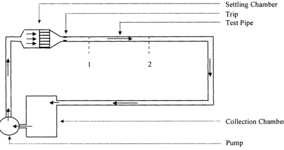
A typical pipe flow apparatus, such as that used by Ptasinski et al. (2001), consists of a pump, a

settling chamber, a trip, a long, straight, horizontal test pipe, and a collection chamber; a

simplified schematic of this is shown in Figure 2.1 below.

- I J · -1 I I

i rip

I -Test Pipe

Collection Chamber

Pumn

Figure 2.1 A simplified schematic of the apparatus used by Ptasinski et al. (2001).

The fluid is sucked out of the collection chamber and driven into the settling chamber by the

pump. The flow is straightened and homogenized in the settling chamber via a mesh or manifold. The flow passes out of the settling chamber and into the test pipe. The trip is situated near the test

pipe entrance to ensure that the flow is fully turbulent. Pressure sensors situated in the test pipe at points and 2 are used to measure the flow pressure gradient along the flow path. The flow then

exits the test pipe and returns to the collection chamber.

batty an R g h am loor

5 3ULLIHIg %-,IIa1IIUUI

(18)

Such an apparatus simplifies the analysis of Equation (2.4) greatly. Taking points 1 and 2 to be

as shown in Figure 2.1, the pressures at these points are measured and therefore known. Because

the test pipe cross-sectional area and the mass flow rate through the system are constants, the flow

velocity through the test pipe must also be constant. In addition, because the tube is horizontal,

the flow height does not change. The net change in flow kinetic and gravitational potential energies between points 1 and 2 must therefore be zero. Also, there are no minor losses between these two points because the pipe is straight and no irregularities are present. Equation (2.4) therefore reduces to

1

(2.5)

p(P2 - pl) = -ghf,

(2.5)

and the head-loss is given directly by the measured pressure difference.

Despite its simplicity, however, this type of apparatus is undesirable in the present study for several reasons. First, pressure is a very difficult flow property to measure; pressure can vary greatly along the flow cross-section, and pressure sensors are expensive, delicate, and difficult to calibrate properly. Second, the use of a pump to generate pressure head in this way accelerates

the degradation of polymer molecules and potentially prohibits the re-use of a single batch of

polymer solution for multiple experiments. Third, no appropriately proportioned space was available for the use of a long, straight, horizontal pipe. It was therefore necessary to design and build a novel, adaptable, low-cost pipe flow apparatus.

2.3 Concept for a Novel Pipe Flow Apparatus

The apparatus described above is one in which the driving energy is known (it is provided by the pump), the mass flow rate is constant, and the flow pressure varies along the test pipe. Because it was desired that the novel apparatus be designed to measure turbulent drag without the use of pressure sensors, however, flow pressure cannot be measured along the test pipe. In order to eliminate the pressure terms in Equation (2.4), then, the novel apparatus was designed such that the flow pressure did not vary along the test pipe.

Additionally, it was desired that the working fluid flow be generated and adjusted without the use

(19)

straightforward method of generating and adjusting pressure gradients on a fluid system, this requirement essentially eliminated pressure-driven flows, and other driving methods were considered. The two rotational geometries discussed in the beginning of this Chapter are wall

driven, but this is not an option for pipe flow. The simplest method of driving a pipe flow without a pump, then, is via gravity. A gravity driven flow requires no special equipment, and can be adjusted by simply adjusting the vertical drop. It should be noted, however, that gravity driven flows do not lend themselves to closed, recirculating systems, because there is no way to

drive the fluid against gravity without a pump.

Finally, it was desired to measure turbulent drag in a simple, reliable fashion, and without the use

of pressure sensors. If the flow is gravity driven, the driving energy is known from the apparatus

geometry. If, in addition, the pressure is invariant along the test pipe, the only unknown term in

Equation (2.4) above is the mean fluid velocity. The flow rate is then the property that must be measured. The only method for measuring flow rate in a closed system such as that discussed in

the previous Section is via a flow meter of some kind. As with pressure sensors, these meters are

delicate and difficult to calibrate. In an open system, however, flow rate can be measured in a very straightforward fashion - the test fluid can be collected in a reservoir as it exits the system,

and the mass of the reservoir can then be measured as a function of time.

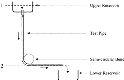
The novel apparatus was therefore designed around system, and the mass flow rate through the system

apparatus is shown in Figure 2.2 below.

1 I I I

I

.4-a gr.4-avity-driven flow through an open was be measured. A schematic of the

Upper Reservoir

Test Pipe

Semi-circular Bend

Figure 2.2 A schematic of the novel

7

pipe flow apparatus. Ipipe flow apparatus.

4 Lower Reservoir [

r-,)*

% 'L J , _ s < _/ I. """""""""""""""""""""""""""""""""""""""""""""""""""""" - -_ - -- _ I , _ , _ _ 4 _ _ o4 _ _ _ v I n J |

(20)

This apparatus consists of an upper reservoir and a lower reservoir, connected to one another by a test pipe. To measure the turbulent drag of a given fluid flow, the upper reservoir is filled with the working fluid and drained into the lower reservoir via the tube. The mass flow rate through

the system is given directly by measuring the mass of the lower reservoir as a function of time.

Taking points 1 and 2 along the flow path to be as shown in Figure 2.2 - the free surface of the

fluid in the upper reservoir and the exit of the tube at the lower reservoir, respectively - the

energy balance as given in Equation (2.4) can be simplified significantly. As discussed above, the flow pressure does not change between points 1 and 2: the pressure at point 1, being at the free surface of the fluid, must be equal to the ambient pressure; the pressure at point 2, being that of a jet exiting to the atmosphere, must also be equal to the ambient pressure. The difference between these two pressures, therefore, does not contribute to a net energy change in the system. Because the mass flow rate through the system is constant, the mean flow velocity at point 1 must be related to that at point 2 by the ratio of the cross-sectional areas normal to the flow at these two points. Because the cross-sectional area at point 1 is substantially larger than that at point 2, the

velocity of the flow at point 1 must be substantially smaller than the velocity of the flow at

point 2; for this reason, the velocity of the fluid at point 1 is traditionally neglected (taken to be zero). For completeness, this term will be taken to be small but non-zero in the present analysis. Finally, taking the height of the tube exit (point 2) as the reference height, the height of the flow at points 1 and 2 are d + Lv and 0, respectively, where d is the depth of the fluid in the upper

reservoir and L is the vertical distance from the tube entrance to the tube exit. Equation (2.4) can now be rewritten

1 )_(A22

1 Al2

1 )

g(d

+

Lv)

=-(ghf +

eminor),

(2.6)

2

p

A22 A 12

where A and A2 are the cross-sectional areas normal to the flow at points 1 and 2, respectively,

h is the mass flow rate of fluid through the system, and all other terms have been defined

previously.

Thus, this apparatus design allows the turbulent drag (in the form of head-loss) to be found for a given working fluid by measuring the mass flow rate through the system. The measurement is simple, reliable, and accurate, and no pump or pressure sensors are used.

(21)

2.4 Presentation of Results

The head loss is typically converted to an average wall shear stress, Tw

w

=

pgh/,

(2.7)

where D and L are the diameter and total length of the pipe, respectively. This value is then scaled with the cross-section averaged flow kinetic energy per unit volume to give the

dimensionless friction factor

f:

If~

2D~ (

ghf

L ) u2(2.8)

f2

L U

2

_,

where U is here the mean fluid velocity within the pipe, defined such that h = pA2U. Note that

this is the Fanning friction factor, not to be confused with the Darcy friction factor; the Darcy value is larger by a factor of 4.

The mass flow rate or average flow velocity within the tube are typically given as a Reynolds

number based on the tube diameter Re:

pUD

4rh

Re=

=

,

(2.9)

17 irDr

where ri7 is viscosity of the fluid.

Experimental results for turbulent drag are presented as plots of

f

against ReD on a logarithmic

scale - i.e. in Moody coordinates - or as plots of f -Y2 against log ReD f ) on a linear

scale-i.e. in Prandtl-Karman coordinates; both forms will be presented here. The friction factor can be measured over a range of Reynolds numbers in several ways. The typical method is by changing the driving pressure, and therefore also the mass flow rate and the Reynolds number. While this

is not an option with the present apparatus, there are two other primary ways in which the Reynolds number can be changed: both the vertical drop, L, and the pipe diameter, D, can be

(22)

2.5 Apparatus Design

It was desired to measure friction factors over a range of Reynolds numbers from 5 x 102 to

5 x 104. For this apparatus, the design parameters were L, the vertical distance between the test

pipe entrance and exit; d, the depth of the fluid in the upper reservoir; D, the diameter of the

test pipe; and L, the total length of the test pipe.

2.5.1 Site Selection

Because it was necessary that the apparatus be designed to fit in the available lab space, a site was selected immediately: a vertical floor-to-ceiling I-beam present in the laboratory provided an ideal structure with which to support the upper reservoir. This eliminated the need for a support

tower of some kind, but necessitated the design and construction of a simple, adjustable device with which to mount the upper reservoir to the I-beam.

This selection of site put constraints on the first design parameter, Lv . In the selected location, there existed both a lower limit (an obstruction approximately 1 m above the floor) and an upper limit (an obstruction approximately 0.5 m below the ceiling) on the value of L, and the apparatus was therefore designed to take advantage of the full available range. This allowed for values of Lv ranging from 0.5 m to 2.5 m.

2.5.2 Upper and Lower Reservoir Selection

Because the upper and lower reservoirs needed simply contain the test fluid before and after it

passed through the test pipe, simple, inexpensive plastic buckets were used.

Because the depth of the fluid in the upper reservoir decreased as the reservoir drained, the

driving energy and therefore the mass flow rate through the system decreased over the course of a given experiment. This effect was minimized by appropriate selection of the bucket used to serve as the upper reservoir. A bucket with a large cross-sectional area was chosen for two reasons: first, so that the maximum depth of water in the upper reservoir (i.e. dmax ) was never larger than

one-fifth of the smallest vertical drop (i.e. L min), and L was then substantially larger than d in

all cases; second, so that the variation of fluid depth with fluid mass within the upper reservoir was minimized.

(23)

The bucket chosen to serve as the lower reservoir was selected such that its volume was

comparable to that of the upper reservoir, but with a smaller cross-sectional area such that it could easily be situated on a scale to measure the mass of the fluid therein.

2.5.3 Test Pipe Selection

Because the flow path included a semi-circular bend, the high performance flexible plastic tubing

was used for the test pipe. This allowed a single length of tubing to be used for each vertical drop.

An overall tube length of approximately 3 m was chosen such that there would be at least 0.5 m

of horizontal tube after the bend for all values of L, such that the bend was present for all experiments, but did not interfere with the exit flow.

Next, tube diameters were selected. In order to insure that the desired Reynolds numbers could

be attained, theoretical predictions of mass flow rate were made for different tube diameters, given the system geometry. For laminar flow, the problem can be solved analytically, and

theoretical relationship between Reynolds number and friction factor is simply given by

16

f = 1(2.10) Re

For turbulent flow, turbulent drag has been thoroughly studied and several comparable empirical

relations have been formulated for the design of turbulent flow systems. One such formula is the Colebrook relation (White 1999):

f-1/2 = + +11) (2.log

2

3.7 2Refl/

2

,

where is the roughness of the tube surface. Equation (2.11) can be iterated in conjunction with

Equations (2.6) through (2.9) to determine the predicted friction factor and Reynolds number for turbulent Newtonian flow through a specified apparatus geometry.

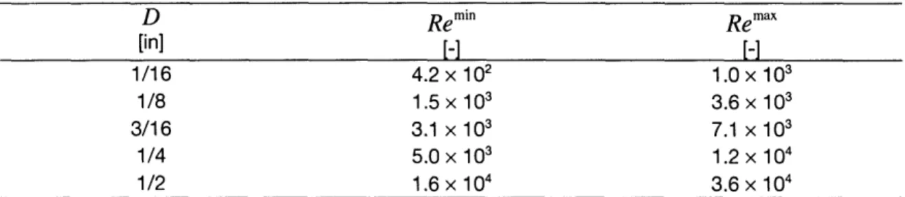
This numerical analysis was carried out for tube diameters from 1/16 in to 1/2 in and for the minimum and maximum values of Lv (Lvmin, 0.5 m, and Lvmax, 2.5 m, respectively). For design

(24)

temperature were evaluated using standard relationships available in the Appendix of

White (1999), and elsewhere. Minor losses were expected to be minimal, and were therefore neglected. The depth of water in the upper reservoir was taken to be 10 cm, a reasonable value for 10 L of water in a tank with cross-sectional area of 0.10 m2. The tubes were taken to be

smooth plastic, with an approximate wall roughness 1.50 x 10-6m. Remin is the Reynolds

number at L m in, and, similarly, Remx is the Reynolds number at Lvmax. Results are shown in

Table 2.1 below.

Table 2.1 Predicted Reynolds number ranges for each tube diameter.

D Remin Remax [in] [-1 [-1 1/16 4.2 x 102 1.0 X 103 1/8 1.5 X 103 3.6x 103 3/16 3.1 x 103 7.1 x 103 1/4 5.0 x 103 _1.2

_{x 10}

4 1/2 1.6x 104 3.6x 104

Although the largest value is slightly lower than the desired maximum Reynolds number, these tube diameters clearly allow for experiments throughout the desired range of Reynolds numbers. The mass flow rate through the system can be found in terms of the Reynolds number, tube diameter, and fluid viscosity from Equation (2.9). Because the goal of this study is to investigate

dilute aqueous solutions, the viscosity of the solution can roughly be estimated to be the viscosity of water for design purposes. Substituting the appropriate values from Table 2.1 above into Equation (2.11) gives minimum and maximum predicted mass flow rates of 5.1 x 10- 4kg/s and

3.5 x 10- kg/s. The former value corresponds to a mass change of approximately 0.1 kg in 200 s, a value that can quite reasonably be measured by hand. The latter value, unfortunately, corresponds to a mass change of 10 kg in only 30 s, and is one that can be measured by hand only with very great difficulty. As will be discussed in Chapter 4, experiments in the higher Reynolds number range (i.e. those with the 1/2 in diameter tube) were attempted in spite of this expected difficulty, but without much success.

A total fluid mass of approximately 10 kg per experiment was decided upon in order to maximize the number of measurements that could be taken at the faster flow rates while minimizing the total drainage time necessary at the slower flow rates. In addition, 10 kg was the largest mass that could be reasonably carried up a ladder in order to fill the upper reservoir.

(25)

2.6 Apparatus Construction

Clear, flexible, plastic (polyurethane) tubes with nominal diameters of 1/16, 1/8, 3/16, 1/4,

andl/2 in, and the necessary fittings (nozzles) were purchased from Small Parts, Inc. The tubes were cut to the appropriate length (3.00 + 0.01 m). The upper and lower reservoirs as well as the Quick-Grip clamps used to hold the upper reservoir stand to the I-beam were purchased from McMaster-Carr. The upper reservoir was fitted with a fixture into which the nozzles for the tubes could be plugged. The simple stand for the upper reservoir was constructed from aluminum stock and bolts available in the lab. An A&D SK-20K Scale with a maximum capacity of 20 kg and a resolution of 0.010 kg was used to measure the mass of the lower reservoir, and a simple digital stopwatch was used to measure time.

2.7 Minor Losses

Minor losses in any pipe flow system occur when irregularities exist in the flow path; examples of

irregularities that incur minor losses are expansions, contractions, valves, bends, and any sort of

obstruction. While some minor losses can actually be quite substantial, e.g. that from a partially closed valve, most are nearly negligible in the flow energy balance. Minor losses are typically given in terms of a loss coefficient K such that the flow energy lost per unit mass to the

irregularity is

1

eminor = KU2, (2.12)

in

2

where U is the cross-section averaged flow velocity entering the area of irregularity; this velocity can be found easily from the mass flow rate through the apparatus and the cross-sectional area of the flow path entering the area of irregularity. The loss coefficient for a given irregularity is generally measured empirically by dividing the pressure drop, Ap, across the irregularity in a horizontal pipe flow by the flow kinetic energy per unit volume flowing through the irregularity,

such that

(26)

Correlations for common irregularities are given in most introductory fluid mechanics texts, e.g.

White (1999).

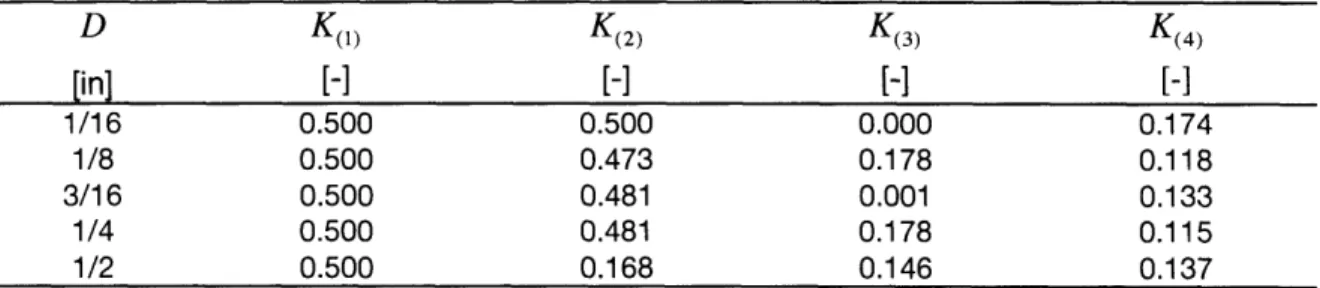
There are four sources of minor loss in this apparatus: the loss due to flow entering the fixture from the upper reservoir; the loss due to the flow contracting slightly from the fixture into the appropriate nozzle; the loss due to the flow expanding slightly from the nozzle into the tube; and the loss due to the flow around the 90 degree bend. The loss coefficients for these four features are given in Table 2.2 below.

Table 2.2 Loss coefficients for the four flow irregularities in the apparatus.

D

[in] 1/16 1/8 3/16 1/4 1/2 K(1) [-] 0.500 0.500 0.500 0.500 0.500 K(2) [-] 0.500 0.473 0.481 0.481 0.168 K(3) []-1 0.000 0.178 0.001 0.178 0.146 K(4) [-] 0.174 0.118 0.133 0.115 0.137 The total energy lost to minor losses can now be evaluated in a straightforward manner and used to find the total head loss due to friction.

(27)

3 Methods

The apparatus described in Chapter 2 was designed and constructed, and the accuracy and

reliability of measurements made therewith were evaluated by performing experiments with tap water and with a dilute solution of polyacrylamide (PAA) in tap water and comparing with previous results. Experiments were then carried out with a dilute solution of partially-hydrolyzed polyacrylamide in synthetic salt water to explore the effect of molecular stiffness on drag reducing effectiveness, and with dilute solutions of hagfish slime in synthetic seawater.

All experiments and measurements were carried out at room temperature, 21 + 1 C, unless specifically noted otherwise.

3.1 Apparatus Validation

The turbulent drag of pure water flows has been thoroughly studied, both empirically and numerically. The predicted friction factor for a given Reynolds number is generally given analytically in the form of an implicit logarithmic relationship such as the Colebrook Relation or graphically in Moody or Prandtl-Karman coordinates.

To establish the accuracy of turbulent drag measurements made with the apparatus, friction factors were measured over the full accessible range of Reynolds numbers for a turbulent flow of tap water, and compared with results predicted by a representative relationship from the literature. Several synthetic high molecular weight polymers are commonly used in turbulent drag reduction studies. One such polymer for which results have been published is polyacrylamide. In order to establish the accuracy polymer drag reduction measurements made with the apparatus, friction factors were measured over a range of Reynolds numbers for several different polyacrylamide

(28)

polyacrylamide were used - Praestol 2500, nominally 0% hydrolyzed and therefore ionically neutral, and Praestol 2540, nominally 40% hydrolyzed and therefore ionically charged; both were

produced by Stockhausen, Inc.

Finally, experiments were carried out with dilute solutions of hagfish slime in synthetic seawater.

3.2 Polymer Solutions

Experiments with polyacrylamide were carried out at polymer concentrations of approximately

100 ppm (parts per million, by mass). Both Praestol 2500 and 2540 were tested in tap water, and

Praestol 2540 was also tested in a synthetic seawater solution. Experiments with hagfish slime were carried out at substantially lower concentrations due to the very limited availability of the

slime. Hagfish slime mucins were tested at a concentration of approximately 1 ppm, and whole

slime at a concentration of approximately 3.5 ppm. Hagfish slime was tested in synthetic seawater only.

3.2.1 Preparation

Praestol 2500 and 2540 were obtained in dry, granular form.

A 1000 ± 5 ppm solution of Praestol 2500 was then prepared by adding 1.00 ± 0.001 g

polyacrylamide solid to 1.00 + 0.005 kg tap water. This mixture was then heated slightly and stirred for approximately one week until the solid was completely dissolved, and then stored for

no more than one week before testing.

To prepare the final solution for experiments, this concentrated solution was combined with an appropriate quantity of tap water and mixed gently but thoroughly to yield approximately 10 kg

of 100 + 0.5 ppm Praestol 2500 in tap water.

The above procedure was repeated to produce 10 kg of 100 + 0.5 ppm solution of Praestol 2540 in tap water. In addition, a solution of 100 + 0.5 ppm Praestol 2540 in synthetic seawater was prepared by substituting synthetic seawater for tap water in the above procedure.

(29)

Hagfish slime was obtained in solution, in 50 mL samples of unknown concentration. In order to determine the approximate concentration of the samples, a small amount of hagfish slime mucin proteins dissolved in de-ionized water was weighed, dried in a vacuum oven, and weighed again. It was found that the mass concentration of the slime mucin proteins was 200 + 50 ppm.

A 5.6 + 1.5 ppm solution of hagfish slime mucin proteins in synthetic seawater was prepared by adding 25.7 + 0.1 g of the 211 + 43 ppm solution of slime mucin proteins in de-ionized water to 944 + 1.0 g synthetic seawater. This solution was stirred gently until mixed, and allowed to sit for at least one hour. The final solution for experiments was prepared by adding an appropriate quantity of synthetic seawater to yield approximately 5 kg of 1.0 ± 0.25 ppm slime mucin proteins dissolved in synthetic seawater, and mixing gently.

The general procedure above was then repeated to yield approximately 5 kg of a solution of 3.3 + 0.9 ppm whole hagfish slime in synthetic seawater.

Synthetic seawater was prepared according to the procedure outlined in Section 3.2.3 below.

3.2.2 Intrinsic Viscosity Measurement

The shear viscosity of even a dilute polymer solution is typically somewhat greater than that of the solvent alone. The contribution of the dissolved polymer to the solution viscosity is generally measured in terms of the so-called polymer intrinsic viscosity, [1], defined such that

n = n ( + Cn]7), (3.1)

where and r70 are the shear viscosities of the solution and of the solvent, respectively.

Approximately 100 mL of each concentrated solution was collected, sealed, and set aside before the remaining solution was diluted to the working concentration. These samples were used in conjunction with a size OB Ubbelohde viscometer to determine the intrinsic viscosities of the polyacrylamides and of the hagfish slime in solution.

Measurements were made and the intrinsic viscosities of the various solutions calculated in accordance with the suggested method outlined by Collins et al. (1973). Further details and results are given in the next Chapter.

(30)

3.2.3 Synthetic Seawater

Synthetic seawater was prepared using Instant Ocean synthetic sea salt, produced by Aquarium Systems. Instructions provided with the Instant Ocean recommended mixing Instant Ocean with water at an initial ratio of 1 cup of solid to 2 gallons of liquid, and then adjusting the quantities in

small amounts until the specific gravity of the solution is between 1.020 and 1.023.

Unfortunately, as Instant Ocean is intended for use in home aquariums, specific information about the molarity of the resulting solution was not available. Because Instant Ocean is intended for simulating a seawater environment, however, one should be able to safely assume that a solution of Instant Ocean in water, mixed in the suggested proportions, should have species content and concentrations similar to ocean water.

For purposes of reproducibility, it was desired to determine the weight concentration of Instant Ocean in tap water that corresponded to the target specific gravity. Several solutions of varying proportions of Instant Ocean and water were prepared and their specific gravities measured using

an Anton Paar DMA 38 Density Meter, and it was found that a solution of 0.0317 g Instant Ocean per 1 g water (i.e. 3.17 weight-percent) yielded a specific gravity of 1.0204 ± 0.0014. All

synthetic seawater solutions for experimentation were prepared by mixing Instant Ocean with tap water in these proportions and stirring until completely dissolved.

All references to "seawater" from now on should be taken to mean synthetic seawater as prepared with tap water and an appropriate amount of Instant Ocean, unless specifically stated otherwise.

3.3 Drag Measurement

As discussed earlier, the apparatus design facilitates simple, accurate measurement of the mass flow rate through the tube. The upper reservoir stand was adjusted to the appropriate height and the tube of the desired diameter was attached to the exit fixture. The lower reservoir was situated

on the scale and the scale was zeroed. The tube was then run around the bend and anchored such

that it would drain into the lower reservoir. The exit of the tube was closed with a plug, and the working fluid was gently poured into the upper reservoir. Finally, the temperature of the working fluid was measured with a standard thermometer and recorded, the stopwatch was zeroed and then started, and the plug was removed from the tube exit. The mass of the lower reservoir was recorded as a function of time at regular intervals, chosen such that at least five data points could

(31)

be collected before the upper reservoir drained completely, and the mass flow rates calculated from these points were averaged in order to account for the decreasing depth of the fluid in the upper reservoir. Values measured with scale and stopwatch were known to within + 0.005 kg and + 0.5 s, respectively, and the temperature was known to within + 0.5 °C. Accuracies of the remaining apparatus parameters are shown in Table 3.1 below.

Table 3.1 Accuracies of parameters describing apparatus geometry.

Parameter Accuracy

L

v ± 0.005 m

d + 0.0005 m

L ±+0.01 m

D unknown

The accuracies of calculated Reynolds numbers and friction factors were derived from the accuracy values given in this Chapter, according to the standard relationship:

(F)2

=

DF

), (x)2

+

aF

(3X2)2 +

+

) (Xn)2,

2a

(3.2)

where the value F is a function of the parameters x, x2, ... xn, and the terms are here the

accuracies of the given value or parameter. It should be noted that Equation (3.2) assumes that the errors in these values and parameters are normally distributed.

The calculated accuracies of Re and f varied depending on the specific values and parameters of the particular polymer solution and apparatus setup in question, but were typically between

I and 2 %.

The exact diameters of the tubes used were unknown. The manufacturer was not able to specify the exact diameters, and the flexible nature of the tube material made the diameters extremely difficult to measure. The diameters were therefore taken to be equal to their nominal values. This will be discussed further in

(32)

(33)

4 Results & Discussion

Intrinsic viscosity and drag reduction results are presented below.

4.1 Intrinsic Viscosity Measurements

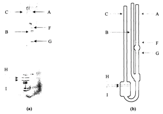
The intrinsic viscosities of the various polymers used for drag reduction experiments were measured in solution with a type OB Ubbelohde viscometer. The basic method of data collection is outlined below. The Ubbelohde viscometer used is shown in Figure 4.1 below. Elements in the schematic are labeled as in the viscometer documentation.

cvk--,

-* .

~:~--

is

k

. . he

C

-+

4-

A

i, 4- F B -- o' - -- G H Iv C B H I (a)

Figure 4.1 Ubbelohde viscometer (a) picture and (b) schematic.

4 - - A

4 ..-- F F- G

... G

(34)

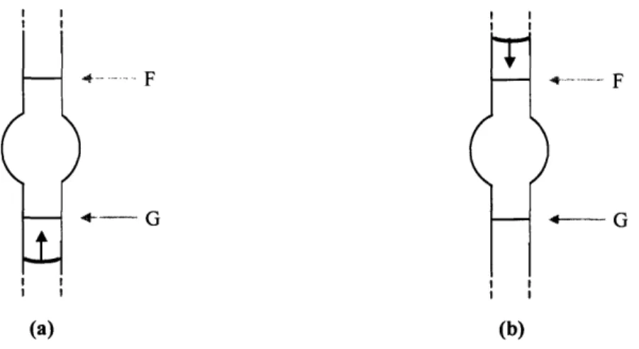
Measurements were made with the viscometer as follows. First, as much of the viscometer as possible was submerged in a constant temperature bath to minimize temperature variation during measurement. Test fluid was then introduced via tube C until the fluid level was between lines H

and J; between 10 and 15 mL of fluid was needed. Approximately 10 minutes was then allowed

for the fluid to reach the bath temperature. Tube B was then plugged, and suction was applied to tube A; this caused the fluid to rise into tube A as shown in Figure 4.2a below. When the fluid

level had risen sufficiently above line F, the suction was released and tube B was unplugged; this

caused the fluid level to begin dropping, as shown in Figure 4.2b below.

T

I I I I

4-oh F s F

X

+

-

G

*-

G

(a) (b)

Figure 4.2. Schematic of the Ubbelohde viscometer test-section. The blue arc and arrow indicate the

location of the fluid free surface and its direction of motion, respectively, while (a) filling and (b) draining. The time it takes for the fluid to pass from line F to line G is known as the efflux time; the efflux

time for a given solution concentration was measured with a stopwatch, and this procedure was then repeated three times for each solution, and for a series of solution concentrations.

This procedure was carried out for each polymer to be used for drag reduction experiments. Data

measured and analysis thereof are shown below for Praestol 2540 dissolved in tap water, as an

example. Results for the other polymers and solutions are tabulated thereafter.

The analysis that follows involves several intermediate measures of viscosity. These are defined as follows: the relative viscosity, r/l, is given by

teff, s 41

1

rel = (4.1)

(35)

where teff s and teff, 0 are the efflux times measured for the solution at a given concentration and

for the pure solvent, respectively; the specific viscosity, 7,P, is simply

(4.2)

r/sp= r1-

1;

the reduced viscosity, 7/d, is given by

7r/sp

C

and the inherent viscosity, 17h, is

1 71inh

=-C

The intrinsic viscosity, [17], of a polymer is then defined to be

(4.3)

(4.4)

[]7] = NM(7 im (ih)

c-+O c-40 (4.5)

It should be noted that while 7r and 17 converge to [17] in the limit as concentration goes to 0, these two measures of viscosity are otherwise not equal. In fact, 17r tends to converge towards [] from above, whereas 17inh tends to converge towards [] from below. Plotting both

17,d

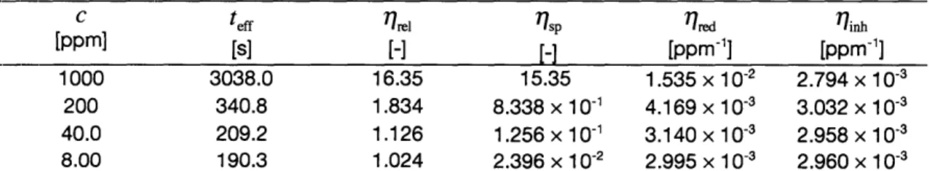
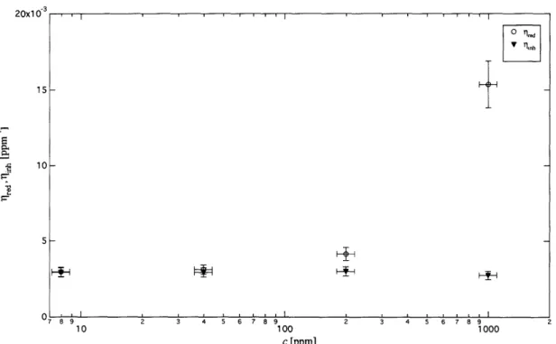
and 17in against c, then, gives the polymer intrinsic viscosity as the single value to which these two curves converge as c vanishes.

Analysis of the data for Praestol 2540 in tap water is shown in Table 4.1 below.

Table 4.1 Analysis of intrinsic viscosity data for Praestol 2540 in tap water.

C teff

17~

7/sp

[ppm] [SI [-] [ -1000 3038.0 16.35 15.35 1 200 340.8 1.834 8.338 x 1 0-1 4 40.0 209.2 1.126 1.256 x 1 0-1 8.00 190.3 1.024 2.396 x 10-2 2 r7red [ppm- 1 .535 x 10 -0169 x 10- 3 3.140 x 10- 3 ..995 x 10- 3 17inh [ppm - 1] 2.794 x 103 3.032 x 10- 3 2.958 x 10'3 2.960 x 10-3

(36)

lU I U 15 10 5 8 9 10

Figure 4.3 Plot of intrinsic

tap water.

2 3 4 5 6 7 8 9 2 3

100 c [ppm]

viscosity data from Table 1 above for a solution

4 5 6 7 8 9

1000

of 100 ppm Praestol 2540 in

It is clear from Figure 4.3 above that 1l/ and rih do indeed converge as concentration

approaches zero; the intrinsic viscosity of Praestol 2540 in tap water is then approximately

3.0

x10-

3 _pm .

Measurements were made and analyzed similarly for the remaining polymers; results are

summarized in Table 4.2 below.

Table 4.2 Intrinsic viscosities of various polymers in solution.

Polymer [n]

[ppm-1 ] Praestol 2500 in tap water 8.5 x 10- 4 + 1.5x 10- 4

Praestol 2540 in tap water 3.0 x 10- 3

+ 1.5 x 10- 4

Praestol 2540 in seawater 8.3 x 10- 4

+ 7.0 x 10-5

hagfish slime mucin proteins in seawater Unknown

whole hagfish slime (both mucin proteins and Unknown fibers) in seawater

Due to the limited quantity of hagfish slime available, the solution of hagfish slime mucin

proteins in seawater was unfortunately indistinguishable from pure seawater. Whole slime was

not tested because of the lack of success with slime mucin proteins, and because it was feared that the fibers would clog the viscometer. Because the solutions used for drag reduction

o n "HH L I IT, I on.. n73 _ 2

(37)

measurements were further diluted from these concentrations by approximately a factor of five, however, it is entirely reasonable to take the viscosity of these solutions to be the viscosity of the solvent.

4.2 Drag Reduction Measurements

Turbulent drag measurements were made over a range of Reynolds numbers for the following

fluids: tap water; a solution of 100 ppm Praestol 2500 in tap water; a solution of 100 ppm Praestol 2540 in tap water; a solution of 100 ppm Praestol 2540 in seawater; a solution of

approximately 1 ppm hagfish slime mucin proteins in seawater; and a solution of approximately

4 ppm whole hagfish slime in seawater.

All drag reduction results are presented in both Moody and Prandtl-Karman coordinates. Error bars were smaller than the symbols used, and are therefore not shown. For consistency, the theoretical curves shown on each plot are the same as those used by Ptasinski et al. (2001). These curves are described by the following relationships: the theoretical laminar flow curve is given

by

16

Rf

=

;

(4.6)

Re the empirical turbulent flow curve is given by

f-1/

2₌

_4.0

_log(Re

_fl/2)

_(4.7)

and the empirical maximum drag reduction (MDR) asymptote is given by

f- 2

= 19.0

log(Re

fl/2

)

_ 32.4.

(4.8)

These three curves are represented in each plot as indicated by the plot legend; consistent symbol

(38)

4.2.1 Tap Water

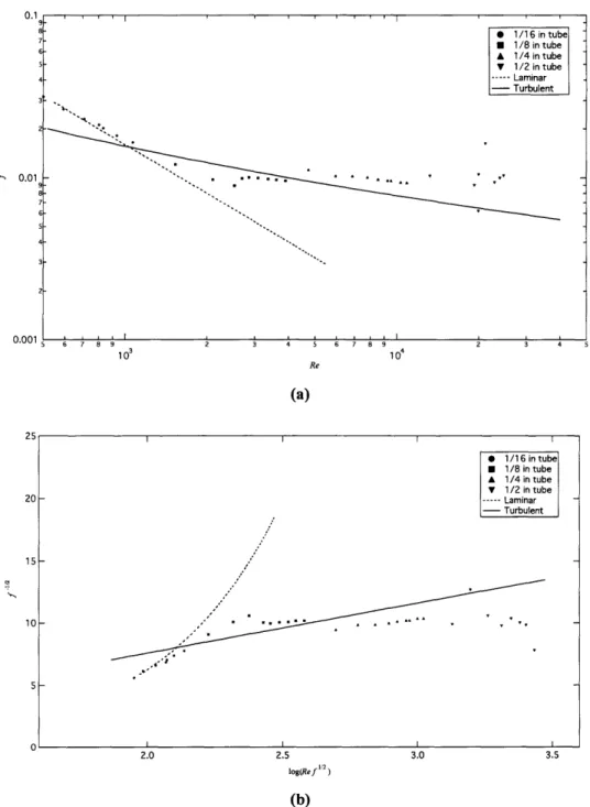
Turbulent drag measurements were made for pure tap water over the full accessible range of Reynolds numbers, and compared against predicted values. The results are shown in Figure 4.4 below. n I 9 6 4 3 2 '- 0.019 8 67 5 34 2 0.001 20 1 5 1 0 5 6 7 8 9 103 2 3 4 5 6 7 89 104 Re (a) 2.0 2.5 log(Ref l ) (b) 2 3 4 3.0 3.5

Figure 4.4 Turbulent drag measurements for tap water in (a) Moody and (b) Prandtl-Karman coordinates.

Calculations were carried out using the nominal tube diameters.

- . I . I Il . lI I . . * 1/16intube * 1/8 in tube A 1/4 in tube 4 ---

~~~~~~

~~~~~~~Laminar

-Turbulent 1/1 6 in tube * 1/8 in tube A 1/4 in tube V 1/2 in tube --- Laminar - Turbulent ,,7 A*~~ I I IO [11

(39)

It is clear from Figure 4.4 above that, other than data measured with the 1/2 in tube, the shape of the data agrees fairly well with the predicted curves; the actual values measured with the 1/8 in and 1/4 in tubes, however, lie somewhat far from the predicted curves. The smoothness of the two data sets implies that the measurements are themselves quite precise, and the fact that the data for the 1/8 in tube is consistently below the predicted curve while the data for the 1/4 in tube is consistently above the predicted curve implies that this is not the result of a large, regular inaccuracy that has not been accounted for; indeed, the magnitude of these errors is well outside of the expected margin of inaccuracy (which is not shown, as mentioned earlier, but is smaller than the symbols). Because the only parameter that differs between these two data sets is the tube diameter itself; then, it seems likely that this error results from the fact that the exact tube diameters differ from the nominal tube diameters.

While both the Reynolds numbers and the friction factor vary with tube diameter, the friction factor, in particular, exhibits an exceptionally strong dependence thereon (fscales with D5

,

whereas Re scales with D-' ; this can be seen by rewriting Equations 2.3.2 and 2.3.3 in terms of

the fluid mass flow rate instead of the mean flow velocity). Very small inaccuracies in tube diameter therefore lead to very large inaccuracies in friction factor.

As discussed in the previous Chapter, it was unfortunately not possible to measure the exact diameters of the tubes. Because the vast majority of the inaccuracy in the data is a result of the inaccuracy in the tube diameters, however, the exact tube diameters must be those values that

scale the data onto the predicted curves. These corrected values were found to be only 1.0 % larger and 3.5 %0 smaller than the nominal values for thel 1/8 in and 1/4 in tubes, respectively.

Data points were recalculated using these corrected values, and the results are shown in Figure 4.5 below. This correction clearly leads to much better agreement of measured data with predicted values. Corrected diameter values will be used in all calculations from now on,

although tubes will still be referred to by their nominal diameters.

In both Figures 4.4 and 4.5, unfortunately, the data from the 1/2 in tube is wildly inaccurate. This

has little to do with the diameter of the 1/2 in tube, and is in fact a result of the fact that the mass flow rate of fluid through the system also the rate of change of the mass of the lower reservoir -was faster than the "refresh rate" of the scale, and therefore these higher flow rates could not be measured reliably. Because of this, no further measurements were made with the 1/2 in tube.

(40)

9 8 7 6 4 2 ,=I 0.019 8 7 6 4 0.001 * 1/16 intube * 1/8 in tube A 1/4 in tube v 1/2 in tube --- Lamrninar Turbulent .~~ ~ 1 _v I I 6 7 8 9 2 3 4 5 6 7 8 9 2 3 4 103 104 Re (a) 25 I I I * 1/16 in tube * 1/8 in tube A 1/4 in tube V 1/2 in tube

~~~~~~~~~~~~~20-

--

Laminar

Turbulent 15 10 _".' Fv tt 0_{5__} , , , , I , , , , I , . . I 1.5 2.0 2.5 3.0 3.5 log(Re f"2 ) (b)

Figure 4.5 Turbulent drag measurements for tap water in (a) Moody and (b) Prandtl-Karman coordinates.

Calculations were here carried out with the corrected diameters for the 1/8 and 1/4 in diameter tubes.

The design and construction of a novel pipe flow apparatus for exploring polymer drag reduction