Behavioral dynamics of public transit ridership in Chicago and impacts of COVID-19

(1)

Behavioral Dynamics of Public Transit Ridership in

Chicago and Impacts of COVID-19

by

Mary Rose Fissinger

B.S., Boston College (2015)

M.S., University of California, Berkeley (2016)

Submitted to the Department of Civil and Environmental Engineering

in partial fulfillment of the requirements for the degree of

Master of Science in Transportation

at the

MASSACHUSETTS INSTITUTE OF TECHNOLOGY

September 2020

c

○ Massachusetts Institute of Technology 2020. All rights reserved.

Author . . . .

Department of Civil and Environmental Engineering

August 17, 2020

Certified by . . . .

Jinhua Zhao

Associate Professor

Thesis Supervisor

Certified by . . . .

John Attanucci

Research Associate

Thesis Supervisor

Accepted by . . . .

Colette L. Heald

Professor of Civil and Environmental Engineering

Chair, Graduate Program Committee

(2)

(3)

Behavioral Dynamics of Public Transit Ridership in Chicago

and Impacts of COVID-19

by

Mary Rose Fissinger

Submitted to the Department of Civil and Environmental Engineering on August 17, 2020, in partial fulfillment of the

requirements for the degree of Master of Science in Transportation

Abstract

Public transportation ridership analysis in the United States has traditionally cen-tered around the tracking and reporting of the count of trips taken on the system. Such analysis is valuable but incomplete. This work presents a ridership analysis framework that keeps the rider, rather than the trip, as the fundamental unit of anal-ysis, aiming to demonstrate to transit agencies how to leverage data sources already available to them in order to capture the various behavior patterns existing on their transit network and the relative prevalence of each at any given moment and over time. In examining year over year changes as well as the impacts of the COVID-19 pandemic on ridership, this analysis highlights the complex landscape of behaviors underlying trip counts. It keeps riders’ mobility patterns and needs as the focal point and, in doing so, creates a more direct line between results of analysis and policies geared toward making the system better for its riders.

This work makes use of two primary methodological tools: the k-means clustering algorithm to identify behavioral patterns, and linear and spatial regression to model metrics of urban mobility across the city. The former is chosen because of its estab-lished history in the literature as a technique for classifying smart cards, and because its simplicity and efficiency in clustering high numbers of cards made it an attractive option for a framework that could be adopted and customized by various transit agen-cies. Spatial regression is employed in conjunction with classic linear regression to capture spatial dependencies inherent in but often ignored in the modeling of urban mobility data.

Chapter 3 of this work identifies the behavioral dynamics underlying top-level ridership decreases between 2017 and 2018 on the Chicago Transit Authority (CTA) and finds that riders decreasing the frequency with which they ride, rather than leaving the system, is the primary driver behind the loss of trips on the system, despite growth in the number of frequent riders using the system for commuting travel. The following chapter applies a similar framework to understand the precipitous ridership drop due to COVID-19 and discovers distinct responses on the part of two frequent rider groups, with peak rail riders abandoning the system at rates of 93% while

(4)

half of off-peak bus riders continued to ride during the pandemic. Chapter 5 uses linear and spatial regression to model the percent change in trips due to COVID by census tract and finds that even when controlling for demographics, pre-pandemic behavior is predictive of the percent loss in trips. Specifically, high rates of bus usage and transfers, along with pass usage, are associated with smaller drops in trips, while riding during the peak is predictive of larger decreases in trips. Chapter 6 presents preliminary thoughts on employing a spatial regression framework on high-dimensional data to learn urban mobility patterns.

This work highlights the insights to be gained from an analysis framework that re-veals the complex behavioral dynamics present on a transit network at any given time. It further connects these behaviors to other rider characteristics such as home location and response to the COVID-19 pandemic, painting a rich picture of an agency’s riders with their existing data and allowing for informed, targeted policy creation. A key finding was that frequent, off-peak bus riders who frequently have to transfer are one of the largest groups of riders and the group most associated with continued ridership during the pandemic. Future policies should recognize that this group uses the system when and where overall ridership is low, and direction of resources away from these parts of the system will disproportionately hurt riders who are most reliant on public transit and therefore have the most to gain from increased investment. The CTA should work in conjunction with other stakeholders to ensure that as public transit ridership recovers from the pandemic, attention is paid not only to those riders who need to be brought back onto the system, but also those who never left it.

Thesis Supervisor: Jinhua Zhao Title: Associate Professor

Thesis Supervisor: John Attanucci Title: Research Associate

(5)

Acknowledgments

This work is indebted to the Chicago Transit Authority. I would like to especially thank President Dorval R. Carter for his continued support and enthusiasm for the partnership between the CTA and MIT. His active engagement with my work and that of my classmates served as inspiration and fuel throughout this process.

This work would also not be possible without Maulik Vaishnav, who answered my endless questions about the Ventra data and provided invaluable insight into the workings of the CTA and the city of Chicago that informed much of this thesis. His genius policy analysis contributed immensely to Chapter 3 and taught me lessons that I will take with me into my career.

Tom McKone and Scott Wainwright additionally provided thoughtful guidance along the way, helpful context in which to situate my work, and willing direction to answers if they themselves could not provide them. Molly Poppe proved to be a reliably active listener and advocate for this work, and I appreciate her immediate and enthusiastic investment in the MIT partnership. Laura De Castro is the glue that holds everything together, and I and everyone at MIT who works with the CTA are deeply grateful for all that she does. Additionally, I would like to thank Jeremy Fine, Paris Bailey, Ray Chan, Bryan Post, Elsa Gutierrez, and Emily Drexler for their conversations and solutions along the way. I want also to express gratitude for every employee at the CTA who works each day to keep the system running, power an extraordinary city, and offer such a successful example of American public transit to the people like me who sit at a computer and crunch the numbers.

To Daiva Siliunas, thank you for sheltering me whenever I came to Chicago. You are a phenomenal host and an even better friend.

At MIT, I would like to express gratitude for the guidance of Jinhua Zhao, John Attanucci, and Fred Salvucci for providing wisdom that improved this work and me as a thinker. I would also like to thank my talented classmates and colleagues for filling the environment with rich and varied public transit knowledge. In particular, Shenhao Wang brought structure and rigor to Chapter 6, Hui Kong offered feedback

(6)

that vastly improved Chapters 3, 4, and 5, and Joanna Moody’s edits to Chapter 4 transformed it into something much better. Lastly, thanks especially to Annie Hudson for the 5PM Tuesday beers at the Muddy that got me through it all.

To my parents, thank you for the support and love that has been the most powerful and important constant in my life. I am incredibly blessed and owe it all to you.

(7)

List of Figures

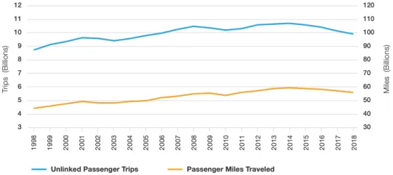
1-1 Yearly Public Transportation Ridership in the United States, 1998

-2018 . . . 18

2-1 CTA Rail Map Network . . . 31

2-2 Number of Jobs in Chicago by Location (Downtown or Elsewhere) . . 32

2-3 Count of Yearly Trips on CTA . . . 33

2-4 Daily Ventra Taps in 2020 with Key Dates from COVID-19 Manage-ment in Chicago . . . 36

3-1 Distribution of Cluster Values for 2017 and 2018 (Part 1) . . . 47

3-2 Distribution of Cluster Values for 2017 and 2018 (Part 2) . . . 48

3-3 Relative Centroid Values by Cluster . . . 51

3-4 Number of Riders By Cluster Group and Observed Behavior Shift . . 53

3-5 Size of Rider Behavior Shifts from 2017 to 2018 . . . 55

3-6 Count of Churned and New Riders by Cluster . . . 58

3-7 Count of Riders Shifting To and Away from Each Cluster . . . 58

3-8 Percent of Non-New Riders in Each 2018 Cluster by 2017 Cluster . . 59

4-1 Daily Ventra Taps by Mode Since First Monday of 2020 . . . 67

4-2 Temporal Distribution of Daily Trips by Mode, Weekend/Weekday, and Time Period . . . 68

4-3 Percent Change in Average Weekly Trips Between Pre-COVID and Early Stage (Left), Between Early Stage and Late Stage (Middle), and Between Pre-COVID and Late Stage (Right) by Community Area . . 70

(12)

4-4 Inferred Home Locations for All Riders (Left) and by Cluster for Most

Frequent Clusters (Right) . . . 74

4-5 Number of Riders in Each Cluster Group by 2018 to 2017 Behavioral Shift . . . 77

5-1 Chicago Regions . . . 91

5-2 Percent Change in Average Weekly Trip Volume by Tract after Stay-at-Home Order . . . 91

5-3 Pearson Correlations Among Explanatory Variables . . . 93

5-4 Residual Analysis for OLS Model with No Region Dummies . . . 102

5-5 Residual Analysis for OLS Model with Region Dummies . . . 102

5-6 Residual Analysis for Spatial Lag Model . . . 109

6-1 Hourly Trips by Mode: Oct. 19 - Oct. 25 . . . 124

6-2 Maximum Hourly Usage by Grid Cell for Each Mode . . . 125

6-3 Average Hourly Usage by Grid Cell for Each Mode . . . 125

6-4 Average TNC Trip Origins by Hour for Weekdays in October 2019 . . 127

6-5 Average TNC Trip Origins by Hour for Saturdays in October 2019 . . 128

6-6 Average Public Transit Trip Origins by Hour for Weekdays in October 2019 . . . 129

6-7 Average Public Transit Trip Origins by Hour for Saturdays in October 2019 . . . 130

6-8 Public Transit and TNC Trip Origin Volumes on Wednesday, October 2, from 8:00-8:15AM . . . 132

6-9 Public Transit and TNC Trip Origin Volumes on Wednesday, October 2, from 6:00-6:15PM . . . 132

6-10 Public Transit and TNC Trip Origin Volumes on Thursday, October 3, from 2:00-2:15AM . . . 133

6-11 Public Transit and TNC Trip Origin Volumes on Friday, October 4, from 6:00-6:15PM . . . 133

(13)

6-12 Public Transit and TNC Trip Origin Volumes on Saturday, October 5, from 2:00-2:15AM . . . 134 6-13 Public Transit Share of Public Transit and TNC Trip Origins on

Thurs-day, October 3 . . . 136 6-14 Public Transit Share of Public Transit and TNC Trip Origins on

Sat-urday, October 5 . . . 137 6-15 Spatial Distribution of Demographic Variables . . . 139 6-16 Spatial Distribution of Land Use Variables . . . 140 6-17 Correlation Heatmap for Demographic and Land Use Variables . . . . 141 6-18 Correlations Between Spatial Covariates and Trip Count Volumes by

Mode and Time of Week . . . 141 6-19 Predicted vs. Real Total TNC Trip Counts for 1 Week - HOD dummies

for Week and Weekend . . . 143 6-20 Hour of Day Coefficients for Each Day of Week and Station Presence

Interaction . . . 148 6-21 Predicted vs. Real Total TNC Trip Counts for 1 Week - Spatially

Lagged Dependent Variable . . . 150 6-22 Predicted vs. Real Total TNC Trip Counts for 1 Week - Spatially

(14)

(15)

List of Tables

3.1 Description of Input Features for Longitudinal Cluster Analysis . . . 45

3.2 Percent of Riders and Trips Belonging to Each Cluster - 2018 . . . . 50

3.3 Change in Cluster Membership Size from 2017 to 2018 . . . 57

4.1 Description of Input Features for COVID Cluster Analysis . . . 66

4.2 Pre-COVID Baseline Behavior Cluster Centers . . . 73

4.3 Percent of Riders from Each Cluster Active by COVID Analysis Period 78 5.1 Independent Variable Descriptions . . . 94

5.2 OLS Regression Results on Percent Change in Average Weekly Trips . 99 5.3 Region Dummies for OLS Regression . . . 100

5.4 Lagrange Multiplier Test Results . . . 106

5.5 Spatial Lag and OLS Model Results . . . 107

5.6 Spatial Lag Variable Impacts . . . 108

6.1 High Dimensional Spatio-Temporal Regression Experiment Design . . 123

6.2 Temporal Model Parameter Estimates . . . 144

(16)

(17)

Chapter 1 Introduction

1.1 Background

As recently as five years ago, the story looked promising for public transit ridership in America. Except for a couple relatively minor dips in trip numbers following the economic recessions in 2001 and 2008, from which public transit ridership recovered in about three years’ time, yearly counts of unlinked passenger trips had enjoyed two decades of steady of growth [American Public Transportation Association, 2020, Mal-lett, 2018]. In 2010, the United States Government Accountability Office delivered a report to the U.S. Senate Committee on Banking, Housing, and Urban Affairs enti-tled "Transit Agencies’ Actions to Address Increased Ridership Demand and Options to Help Meet Future Demand" [Wise, 2010]. The report notes that ridership growth between 1998 and 2008 outpaced the growth in service provision for all modes — light rail, heavy rail, and bus — and attributes the growth in ridership to population increases, employment growth, higher prices for gasoline and parking, as well as addi-tional measures taken by individual agencies, such as the creation of partnerships with local businesses to encourage commuting by public transit. As the title suggests, the report is primarily concerned with recommending changes to public transportation funding that could best help transit agencies meet a continued growth in demand.

Just one decade later, it is hard to imagine such a time in the public discourse surrounding mass transit in America. A few years ago, as it became clear that the dip

(18)

Figure 1-1: Yearly Public Transportation Ridership in the United States, 1998 - 2018 Source: 2020 APTA Fact Book

in ridership from 2014 to 2015 was not a blip but rather the beginning of a sustained downward trend, the conversation around mass transit in the U.S. changed markedly. News publications and transit blogs around the county adopted language that ranged from colorful to apocalyptic to describe the current state of affairs. The Washington Post used a headline quoting experts describing the situation as an "emergency" [Siddiqui, 2018] while The Los Angeles Times ran a story describing the city’s bus system as "hemorrhaging" riders [Laura J. Nelson, 2019].

These stories in turn quickly came to feel like historical documents after March of 2020 and the spread of the COVID-19 virus in America. As schools shut, businesses closed down or turned to remote work, and state and local governments urged people to remain home as much as possible and avoid crowded indoor areas, public transit ridership plummeted across the world [Transit, 2020]. According to the mobile app Transit, which allows users to track locations of trains and buses in their city, demand for public transit as measured by use of their app was down 75% in the month of April. Headlines on articles addressing transit ridership in America spoke about the end times for mass transit: Time Magazine published an article in July whose title asserted that "COVID-19 Has Been ’Apocalyptic’ for Public Transit" [De la Garza, 2020] and Forbes published a piece posing the question "Will COVID-19 Sound The

(19)

Permanent Death Knell For Public Transit?" [Templeton, 2020].

The sudden and precipitous drop in ridership that occurred in US cities made the fluctuations in trip numbers over the previous few decades seem incredibly stable. The temporal and spatial distribution of trips within cities changed shape almost overnight, and many things that had once felt like accepted facts about transit usage in a city had to be re-investigated and re-learned.

As cities and transit agencies across the country are re-grouping and attempting to learn all they can about what is likely to be a new normal of significantly reduced transit ridership for some time, they have an opportunity to rethink and enrich how they measure and track ridership on their systems. This work offers one potential avenue for doing so. Specifically, it puts forth a ridership analysis framework that centers around the rider instead of around trip counts. It demonstrates the usefulness of such a framework for, first, understanding the mobility needs of riders at any given time, for example during a global pandemic, and, second, crafting policy based on these needs.

1.2 Motivation

Public transportation ridership analysis in the United States has traditionally cen-tered around the tracking and reporting of the count of trips taken on the system. These numbers can be disaggregated spatially to the zone, census tract, line, or stop, or disaggregated temporally to weekends, weekdays, peak periods, and off-peak pe-riods. They can be normalized by capita or by revenue vehicle mile or available capacity, and they can be tracked across months and years. Such analysis provides valuable information about the health of public transit systems within and across US cities and how this is trending over time. The value of analysis based on counts of trips will never be supplanted, but it is incomplete. By using the passenger trip as the fundamental unit of analysis, it obscures the reality of a city as a place full of people who are living, working, visiting, and, to various extents, making use of the public transit system to get them where they need to go. A ridership analysis framework

(20)

that keeps the rider, rather than the trip, as the fundamental unit of analysis, on the other hand, seeks to understand the patterns in which trips across hours, days, or months and across neighborhoods, lines, and modes are tied to an individual person. Its aim should be to capture the patterns of behavior that exemplify how people typ-ically use their transit network and the relative prevalence of these behaviors. This type of analysis re-centers the question on the people rather than the trips, and leads to answers that are focused around “who?” instead of “how many?” It keeps riders’ mobility patterns and needs as the focal point and, in doing so, creates a more direct line between results of analysis and policies geared toward making the system better for its riders.

1.3 Research Aims

The primary aim of this work is to demonstrate to transit agencies how to leverage data sources already available to them in order to better understand who their riders are and how they use the system. I furthermore seek to show how this knowledge can form the baseline of deeper analysis that addresses a few crucial questions facing American transit agencies today, and how, by keeping the rider as the fundamental unit of analysis, the results can directly inform policies aimed at riders. This work was begun in pre-pandemic times and as such, I first demonstrate how to track changing behaviors across years to uncover the behavioral dynamics underlying relatively minor top-level changes in trip counts. Next, I leverage this framework to explore the distinct ridership responses to the COVID-19 pandemic by behavior group and use this rider-centric knowledge to craft policy recommendations for ridership recovery. Then I employ linear and spatial regression to identify the behavioral and demographic traits most predictive of COVID-related ridership loss. Lastly, I offer some initial thoughts on how to better understand the urban mobility landscape of a city by leveraging high dimensional data to capture the dynamics among multiple modes’ usage patterns.

(21)

1.4 Data and Methods

This work was sponsored by and done in conjunction with the Chicago Transit Au-thority (CTA) and thus uses Chicago as the case study for all analyses. All data on public transit usage comes from the CTA’s account-based fare payment system Ventra, but the framework could be applied by any agency with a widely used smart card fare payment system in place.

The primary methodology employed for the identification of key behavioral pat-terns on the CTA’s network was the k-means algorithm applied to a dataset in which each point to be clustered was a single Ventra card whose behavior was captured by a vector of unit-standardized attributes summarizing key aspects of the card’s us-age, such as the percent of trips taken during peak hours or the average number of weekly trips taken on that card. The k-means algorithm was chosen because of its established history in the literature as a technique for classifying smart cards, and because its simplicity and efficiency in clustering high numbers of cards made it an attractive option for a framework that will ideally be adopted and customized by various transit agencies. This work’s contribution lies not within the realm of rider segmentation methodologies, but in establishment of a framework for segmentation that is accessible to transit agencies and can easily serve as the foundation for deeper analysis and informed policy creation.

The other methodology employed in this work is that of linear and spatial regres-sion. Spatial regression models, and particularly spatial lag models, are employed as alternatives to linear regression that should be explored in the modeling of mobility data that is located in space. The use of such models in ridership analysis within a single city has been limited, and this work does not seek to definitively establish its usefulness in the urban mobility context, as much more research is needed on this front, but it does offer it as a model worth considering, at least in the situations in which I employ it. The first such situation is a model in which aggregate traits of individuals assigned to a census tract based on inferred home location are used to explain ridership changes in that tract. Here, the likely tract spillover of transit use

(22)

due to people using multiple stops near their home, as well as the interconnectedness and resulting lack of independence of the network in general, motivated an explo-ration of a spatial lag model that used nearby ridership loss to explain tract-specific transit ridership loss. One can easily imagine other models of trip volume or ridership changes by geographic area that could benefit from the inclusion of spatially lagged dependent or independent variables. One such example is from the final analytical chapter of this work, which is motivated by the hypothesis that TNCs are in com-petition with public transit systems, and seeks to provide a set of models that can be used to explore the relationship between usage of the two modes across spatial and temporal dimensions. A straightforward way to explore this question is to model TNC trips as a linear combination of public transit trips in and around the TNC trips’ origin locations. Such a model involves a spatial lag of public transit usage. Capturing the dynamics between modes is a situation that could likely benefit from exploration of spatial regression models, definitions of “neighborhoods,” and other related topics. This work begins to explore these questions.

1.5 Organization of Thesis

Chapter 2 provides background on relevant topics, specifically public transit ridership behaviors in America, the city of Chicago and the CTA system, and the COVID-19 pandemic and the response of transit agencies and riders across the United States.

Chapter 3 offers a framework for transit agencies with account-based fare systems to capture changing behavior dynamics on their systems using smart card clustering on data from multiple years. The CTA is used as a case study, with the data coming from their account-based Ventra system. The behavior changes on the system from 2017 to 2018 are identified and summarized, and then used to pinpoint particular rider groups of interest, who are then investigated in greater depth, using the fact that the Ventra system is rich with data that can be layered onto each card at any point in the analysis. Specifically, the additional analysis at the end of Chapter 3 is performed in order to more deeply understand the impacts of the January 2018 fare

(23)

increase on the CTA system.

In Chapter 4, the same clustering technique is applied (in a slightly modified fashion) to establish the baseline behaviors present on the CTA system in the months just prior to the stay-at-home order issued in Chicago in response to the COVID-19 outbreak. Ridership data from the beginning of the stay-at-home order and from two months after is then analyzed to paint a picture of how the pandemic has affected transit ridership in America’s third largest city. This section concludes with policy recommendations for the CTA in light of the findings.

Motivated by the findings from Chapter 4, Chapter 5 employs a different method-ology to understand the factors associated with the steepest declines in transit rid-ership during the COVID period when compared with the baseline. This section employs classic linear regression as well as spatial regression models to quantify the relationship between demographics and baseline ridership behavior as the explanatory variables and ridership decline as the dependent variable at the census tract level.

Chapter 6 presents preliminary work applying spatial regression concepts to higher dimensional data and begins to explore models that incorporate both the space and time dimension to capture the dynamics of Transportation Network Company (TNC) trips in Chicago. This chapter also lays out ways that this structure could be used to more deeply understand the extent to which TNC ridership is related to transit ridership.

Chapter 7 summarizes the findings and offers concluding thoughts regarding rec-ommendations for the CTA and directions for future work.

(24)

(25)

Chapter 2 Background

This work is motivated by the idea that a deep and continually evolving understanding of how public transit riders make use of their cities’ transit systems is a crucial part of providing good service as a transit agency. Analyses of trip counts tell an incomplete story about the state of transit ridership. Beneath these trip numbers are thousands or millions of people moving about their city, living their lives. Some of them have no other option but to use mass transit. Some use it only to commute, opting for other modes on the weekends or in the evenings. Some use it every day, others once a month. From only aggregate trip counts, one cannot deduce the set of behaviors existing on a system. Yet, knowing these behaviors can inform policies in very valuable ways. Policies aimed at increases in ridership or revenue will be more effective if the target is not merely "more trips" but a person whose mobility needs and challenges are well-understood. Furthermore, if several dominant behaviors can be uncovered, more targeted policies can be directed to each in turn. Transit agencies can meet riders where they are, and then get them where they need to go.

This is not novel thinking — transit agencies have understood this for a long time. But up until recently, their primary method of learning about their riders was surveys, which capture ridership behaviors at a (often very brief) snapshot in time. Longitudi-nal tracking of riders via surveys is expensive, and the validity of the conclusions that can be drawn is sensitive to the sample that is reached and the accurate reporting on the part of the survey takers. While these methods undoubtedly provide valuable

(26)

insights, in part because they have the benefit of capturing rich demographic data along with ridership behavior, the picture they capture of an individual’s ridership behavior is limited, either in terms of detail or duration.

With the emergence of Automated Fare Collection (AFC) smart card technology, however, transit agencies can now connect each trip to a fare card, and observe behaviors on cards that are used for an extended duration. In cities such as Chicago, where the fare payment system is account-based, meaning that even replacement cards can be tied to the same person, the implications are especially powerful. Multi-year ridership trends can be analyzed in terms of underlying changing behaviors, weighing these against volumes of churned riders versus new riders. The impacts of service changes or disruptions can be looked at through the lens of the people affected. Changes to fare policies can be evaluated based on which groups prove most or least elastic. In short, transit agencies now have the ability to more fully understand and meet the needs of the riders they serve.

In the next section, I will offer a review of work that has looked at travel behaviors among public transit riders and work that has studied changes in these behaviors over time. Next I will offer some context on the city of Chicago and CTA system, as that will be the subject of the case studies in this work. Lastly, I will give background on the COVID-19 pandemic, which motivates the analysis in chapters 4 and 5, and explain the ways in which transit agencies, riders, and analysts had responded to the outbreak at the time of this writing.

2.1 How Americans Use Public Transit

Within the realm of travel behavior research, the primary question for the past several decades has been that of mode choice: what makes someone choose one mode over the other? The methodology employed to answer this question is typically a logit model that takes in the riders’ demographics and the trip’s attributes for each mode and outputs the mode that such a traveler would most likely choose. Implicit in this is the idea that individuals make several trips throughout the course of the day, some of

(27)

which may be on public transit, some via private automobile, some using a rideshare service, etc. These models try to capture the context in which someone lives their life and makes travel decisions. The insights such studies can provide are incredibly valuable, as they shed light on the factors riders weigh before setting off on their mode of choice, but the downside is that these models are incredibly data-intensive, requiring information on the decision-maker and each of the travel modes available to her. Studying travel behavior as observed on only a single mode removes much of this rich context but is, with smart card data, readily possible for public transportation agencies. Looking at only public transit ridership behavior can by itself communicate a lot about a person and, coupled with knowledge about how much daily travel the average person engages in, give us a good idea of the extent to which people are using mass transit for all or most of their travel needs.

The mode choice literature helps inform decisions about how to entice more people and trips onto public transit— an extremely important goal, but not the sole objective of a public transit agency. How people currently use the system contains a wealth of information regarding the mobility needs of riders, and understanding these needs so that they can be best met should be an equally important, if not more important, goal of public transit agencies. Thus, an understanding of existing public transit rider behavior is crucial. Furthermore, insight into how these behaviors change over time can shed light on where transit systems need to become more competitive, and where resources should be invested.

Capturing predominant public transit ridership behaviors has received less atten-tion than understanding factors driving mode choice, or determining the demographic profile of transit riders, but with the advent of AFC technology, the question has gained more attention. In Chapter 3 I provide a literature review specifically on how smart card data has been mined to uncover transit ridership behaviors, but none of the studies use data from an American city, so here I will present details on how we currently understand Americans to use public transit and how that is changing over time.

(28)

entitled "Who Rides Public Transportation: The Backbone of a Multimodal Lifestyle" drew on ridership reports from 163 transit systems in the U.S. that surveyed over 650 thousand riders in total [Clark, 2017]. This report found that fully half of all respondents used public transit five times per week. It also found that half of the survey respondents’ most typical transit trips involved a transfer. Among all riders, 29% had been using transit for under two years, and 53% had been using transit for more than five years. Rail riders were more likely to be long-term users of mass transit than bus riders.

TransitCenter’s 2016 report "Who’s On Board" summarized findings from focus groups and online surveys of public transit riders in 17 large and medium-sized cities [Higashide, 2016]. The report found three general behaviors to be predominant on public transit systems: occasional riders, commuters, and all purpose riders. The latter group was most prevalent in cities with strong transit networks offering frequent service to many destinations. This report stressed that all riders were sensitive to transit quality and that the traditional distinction of "choice" and "captive" riders was detrimental.

Using a similar methodology, TransitCenter followed this report up three years later with "Who’s On Board 2019: How To Win Back America’s Transit Riders" [Higashide and Buchanan, 2019]. In it, they determine that declining public transit ridership is driven by people scaling back their use of public transit systems and largely replacing trips with private vehicles, rather than abandoning mass transit altogether. This was reflected in the fact that more riders fell into the "occasional" category than had in 2016.

Despite the outcry over declining public transportation ridership over the past few years, few studies besides the TransitCenter reports mentioned above have examined the behavioral trends underlying these declines. Chapter 3 of this thesis outlines a framework for how transit agencies with access to smart card data can leverage it to answer the same questions answered by the 2019 TransitCenter report: Who is on board their buses and trains, and how are those people shifting their behavior over time? Our analysis demonstrates that many of the nationwide findings from

(29)

TransitCenter’s report hold in Chicago as well, with overall ridership declines being driven by people using the system less, rather than fewer people using the system at all.

2.2 Chicago and the CTA

The case studies in this work all focus on the city of Chicago, as all of the public transit ridership data comes from the CTA’s account-based fare payment system, Ventra.

Chicago is located on the coast of Lake Michigan in Illinois and is the third largest city in the United States with a population of 2.6 million, surpassed only by New York City (8.3 million) and Los Angeles (4 million). The CTA is the second largest transit agency in the country behind the Metropolitan Transportation Authority (MTA) in New York in terms of unlinked passenger trips in 2018. Broken out by mode, the CTA provided more trips on heavy rail than any agency other than the MTA and the Washington Metropolitan Area Transportation Authority (WMATA) in 2018, and provided more bus trips than all agencies other than the MTA and the Los An-geles County Metropolitan Transportation Authority (LACMTA) [American Public Transportation Association, 2020].

Outside of the CTA, the Chicago metropolitan area is also home to Metra, the largest commuter rail network outside of the New York City area as measured by unlinked passenger trips, and Pace, a large suburban bus and regional paratransit network. These services exist to complement rather than compete with the CTA, however, and largely bring people from the suburbs into the city or to other areas outside the city. Within the city boundaries, the CTA is the primary provider of mass transit services, and thus analysis using CTA data provides a nearly complete picture of public transit usage in the urban area.

Public transit has been an integral part of Chicago for a long time, with the first rapid transit line opening in 1888. The unique structure of the rail network gave the downtown core of the city its now official name — "The Loop." The CTA’s eight rail

(30)

lines are arranged in a spoke-hub formation, all feeding into the dense downtown area (except the Yellow line, which acts as a feeder branch to the Red and Purple lines in the north). Five of the seven lines that reach the downtown area traverse at least some portion of the 1.79 mile long elevated loop of rail tracks running above Lake Street in the north, Wabash Avenue in the east, Van Buren Street in the south and Wells Street in the west. The other two lines— the Blue line and the Red line — are underground at this point. Figure 2-1 shows the layout of the CTA rail network.

This network structure has contributed to the continued concentration of jobs in and around the Loop. More than half of Chicago’s jobs are located in the downtown area, and the total number of downtown jobs as well as the proportion of jobs located in downtown has been growing since 2010 (Figure 2-2). Patterns of usage on the CTA’s rail system reflect its role as a connection to jobs: in 2019, just over half of all Ventra card taps on CTA’s rail system occurred between the hours of 6AM and 10AM or between 4PM and 8PM on weekdays.

The bus network structure, on the other hand, largely reflects the city’s grid layout, with most routes running north-south or east-west, many along a single street. Bus ridership on the system also exhibits peak patterns, but to a lesser extent than rail. About 45% of Ventra card taps of bus occurred during weekday peak hours during 2019.

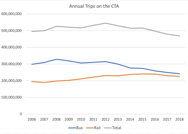
Ridership by year for each mode between 2006 and 2018 is shown in Figure 2-3. While bus ridership has declined each year since 2012, rail mostly continued to grow ridership until 2015. Since then, until the COVID pandemic, total ridership on the system had declined by about 3% yearly, with slightly steeper losses coming from bus rather than rail [Chicago Transit Authority, 2020b]. This is largely in line with nationwide trends in transit ridership, which have been declining since a peak in 2014 [American Public Transportation Association, 2020].

This work began as an effort to explain the CTA’s ridership decreases through the lens of changing individual behaviors. This topic is the focus of Chapter 3 and explores the system’s changing behavioral dynamics between the fall of 2017 and the fall of 2018. Several months after that analysis was completed, however, the

(31)

COVID-Figure 2-1: CTA Rail Map Network

19 pandemic abruptly and dramatically changed daily life for nearly everyone in the world. One element of these changes was people’s travel needs and behaviors.

(32)

Chap-Figure 2-2: Number of Jobs in Chicago by Location (Downtown or Elsewhere) Source: Chicago Sun Times

ters 4 and 5 of this work build off the foundations set forth in Chapter 3 to capture the heterogeneous individual behaviors underlying the massive drop in overall transit trips occurring in Chicago due to the pandemic. Before concluding this chapter, I provide some context on the timeline of the COVID-19 pandemic and what we know about reactions of transit agencies and riders as of July 2020.

2.3 The COVID-19 Pandemic

At the time of this writing, the United States is four months removed from the initial escalation in COVID-19 cases that occurred in the second half of March. We now know that the virus is spread primarily via respiratory droplets, such as those produced when someone coughs, sneezes, or talks, and that people exhibiting no symptoms can still spread the virus [Center for Disease Control and Prevention, 2020a]. There is still much that is unknown about the virus, however, including how unsafe an activity like riding public transit really is for the general population. The body of research on that is growing, and a brief summary of it will be provided here, along with accounts

(33)

Figure 2-3: Count of Yearly Trips on CTA Source: Chicago Open Data Portal of transit ridership responses across the country.

In April, an MIT economics professor published a study claiming that the New York City subway was “a major disseminator—if not the principal transmission vehi-cle” of the disease in the city and the reason the outbreak was so much worse there than elsewhere in the country [Harris, 2020]. His methodology, which involved over-laying declines in subway ridership with infection rates by zip code, quickly drew many critics, who noted his failure to account for any of the obvious cofounders, such as the decline in activities that was driving the decline in transit use [Bliss, 2020]. They also noted that many zip codes with the highest density of transit stations had some of the lowest infection rates [Levy, 2020]. Transit analysts, epidemiologists, and mathe-maticians alike have concluded that the paper provides no concrete evidence that the subway explains why the outbreak was so much worse in New York than elsewhere in the country in the early days of the pandemic [Sadik-Khan and Solomonow, 2020].

(34)

Since this paper, several other studies have provided evidence that subway systems are not, in general, responsible for a significant portion of disease spread. Epidemi-ologists found that in Paris, none of the 150 identified coronavirus infection clusters between early May and early June were traced to public transit usage or transmission [Berrod, 2020]. Likewise, researchers investigating the outbreak in Austria in April and May found that none of the 355 clusters could be connected to transit [Austrian Agency for Health and Food Safety, 2020]. Furthermore, several cities, particularly in Asia, with transit use on par with or higher than New York’s and smaller declines in that usage saw outbreaks that were much more successfully contained [Mahtani et al., 2020]. Hong Kong, for example, had only 1,655 confirmed cases as of this writing or about as many as Duplin County, North Carolina, whose population is just over 59,000, compared with Hong Kong’s 7.5 million [Johns Hopkins University and Medicine, 2020]. Japan, home to the world’s busiest rail network in Tokyo, along with several other major transit systems, has had just over 25,000 confirmed cases compared to the U.S.’s 3.8 million.

While there is growing evidence that public transit systems are not a unique evil in terms of risk of transmission, there is no question that Americans with the option to stay home or use another mode have abandoned it in droves. According to the mobile app Transit, public transit usage was down 77% across the country [Transit, 2020]. The app surveyed the remaining riders and found that they were overwhelmingly (92%) using transit to get to work, and that they were predominantly women of color and 70% of them made under $50,000 a year. Meanwhile, Transit app users in higher paying jobs had been able to shift to working from home. The Eno Center for Transportation analyzed news reports from transit agencies across the country and showed that the drop in transit ridership due to COVID differed significantly by mode, with commuter rail lines seeing the largest drops, followed by urban heavy rail, and then bus [Puentes, 2020]. The difference between commuter rail and bus is stark, with commuter rail ridership down more than 90% in many places, while major bus systems were maintaining up to two-thirds of their baseline ridership. These findings are consistent with those from the survey of Transit app users, as it is well-established

(35)

in the literature that bus riders more likely to be lower income than rail riders [Maciag, 2014].

Transit agencies have responded to the disease and resulting drops in ridership in various ways. Many have significantly reduced their service in order to save money and accommodate staff shortages. New York City’s MTA cut subway service by 25%. WMATA in Washington, D.C. shut down 19 rail stations in response to the pandemic in March, reopening them at the end of June [Washington Metropolitan Area Transit Authority, 2020]. The San Francisco Municipal Transportation Agency (SFMTA) closed all subway stations and replaced all Muni Metro and light rail routes with buses in order to “redirect custodial resources to other, higher-use facilities,” specifically those on routes connecting people to essential jobs and services [Fowler, 2020]. The CTA, on the other hand, made no permanent service cuts despite drops in ridership around 80%, canceling trips only as a result of staff shortages. The CTA also replaced 40-foot buses with 60-foot buses on certain routes that maintained particularly high ridership [Chicago Transit Authority, 2020a]. Aside from changes to service volumes, many transit systems have implemented rear-door boarding for buses to limit passenger contact with operators, rendering bus travel essentially free in these cities. Several have also authorized their bus drivers to maintain capacity caps on buses. In addition, nearly all have increased communication about how to ride safely during COVID, suggesting or requiring masks, advising maintaining a safe distance between passengers, and recommending frequent hand sanitation, among other guidelines.

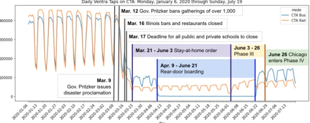
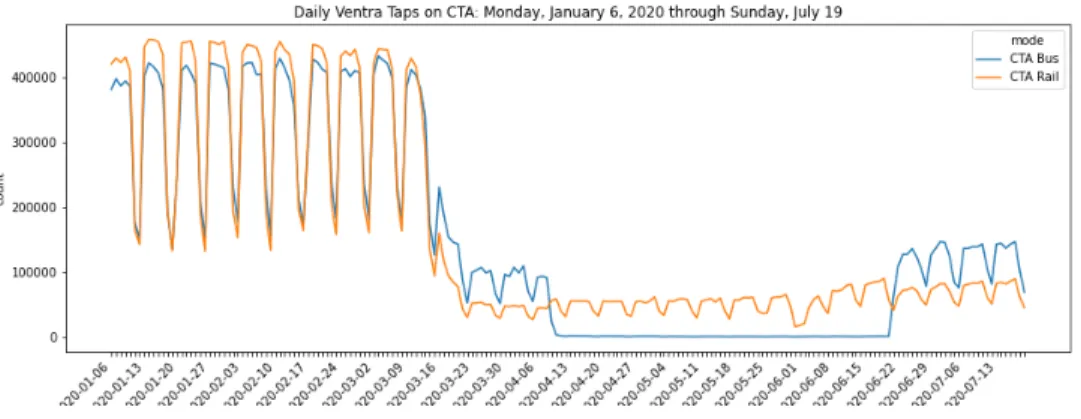
Figure 2-4 shows the daily count of Ventra taps by mode on the CTA from the start of 2020 through July 19, along with key dates in Chicago’s management of the disease spread. Although a Chicago woman on January 24 became the second confirmed case of COVID-19 in the United States, the city, like the rest of the country, maintained business as usual until the early part of March. On March 9, the Governor of Illinois, J. B. Pritzker, issued a disaster proclamation, allowing the state to take advantage of additional state and federal resources to fight the disease. Over the next two weeks, in quick succession, the governor banned gatherings of over 1,000 people,

(36)

ordered all bars and restaurants closed, shut down public and private schools, and on March 21, issued a stay-at-home order [Tribune staff, 2020]. Over the same time frame, the number of rides occurring on the CTA dropped by more than 80%. On April 9, the CTA implemented rear-door boarding on buses, leading to effectively free bus service in Chicago. On June 3, after two and a half months, the stay-at-home order was lifted in Chicago as part of "Phase III" of reopening, which allowed some non-essential businesses to resume operations with capacity limitations [Munks and Anderson, 2020]. Restaurants and coffee shops were permitted to allow outdoor dining, and personal services such as hair salons reopened [NBC Chicago, 2020a]. On June 26, Chicago moved on to Phase IV, which allowed indoor dining at restaurants as long as tables were more than six feet apart, museums were permitted to operate at 25% capacity, and gatherings could occur of up to 50 people, up from 10 in Phase III [NBC Chicago, 2020b].

Figure 2-4: Daily Ventra Taps in 2020 with Key Dates from COVID-19 Management in Chicago

Source: Chicago Tribune, City of Chicago

At the time of this writing, despite being deeply uneasy about the massive revenue drops they are are sure to see for some time, transit agencies are still largely following the suggestions of the CDC and urging riders not to travel unless necessary, so that public transit is as safe as possible for those who need it [Center for Disease Control and Prevention, 2020b]. Eventually, however, transit agencies will need to recover a

(37)

significant portion of their baseline ridership; otherwise, U.S. cities will be gridlocked with private vehicles as people begin moving again. Charting a path forward will require an understanding of who riders were before the pandemic, how their travel behavior shifted in response, and what this information tells us about their mobility needs and the challenges to bringing them back on board. Chapters 4 and 5 of this work use Chicago as a case study to examine the differential impacts of the pandemic on the ridership of a few key groups, and Chapter 4 uses this analysis to craft a multi-pronged policy approach to meet the mobility needs of riders using the service during the pandemic, to get riders back on buses and trains, and to help the CTA be more reflective of the needs of its riders going forward.

(38)

(39)

Chapter 3 Customer Segmentation Framework

The introduction of account-based automated fare collection technology has given transit agencies a new level of depth in their data, allowing for deeper analysis and understanding of the underlying ridership trends present on their system. Whereas before, most transit agencies could only quantify the number of trips made by time of day, day of week, mode, route, or stop, now they can quantify the number of trips made by person, as well as the spatio-temporal distribution of those trips. This allows and, I would argue, demands full recognition of the fact that a transit system is built for people, and that every trip occurs because of the person who decided to make it. This section will demonstrate how to leverage AFC data to uncover how behavior trends are driving top-level ridership changes. The framework presented here will enable transit agencies to answer questions such as whether a ridership decline was due more to riders churning from the system altogether or decreasing the number of trips they took. Which ridership behaviors are most stable? Most unstable? Having identified some key behavior groups of interest, what else can we learn about these riders? And finally, how can we use these insights to inform policy analysis?

3.1 Background

Since the emergence of AFC data, a robust literature on methodologies for mining this data for ridership behavior patterns has emerged. This particular work draws heavily

(40)

from that of Basu, who used k-means to cluster cards from Hong Kong’s Mass Transit Railway (MTR) system [Basu, 2018]. He used one month of data and characterized ridership using both temporal and spatial features with the goal of allowing MTR to target system information to only the riders for whom that information was relevant. The literature on this topic has grown to cover not only a large range of clustering methodologies but also types of systems analyzed and sets of input features. I will touch on only some of them here.

Many of the studies in this body of literature leverage unsupervised learning al-gorithms to uncover patterns in the data. The two most popular within this body of work are k-means and Density-Based Spatial Clustering of Application with Noise (DBSCAN), and they are applied to a variety of different types of input data at various steps in the customer segmentation process. Morency et al., for example, apply k-means in a comparison of just two individuals, and use the algorithm to un-cover days of travel with similar patterns [Morency et al., 2006]. Agard et al. use k-means along with Hierarchical Agglomerative Clustering (HAC) on binary features indicating day of week and time of day to explore the relationship between temporal ridership patterns and fare type [Agard et al., 2006]. To separate infrequent from frequent passengers, Kieu et al. apply k-means to the number of trip chains evident from card usage, and then apply DBSCAN to the frequent group to refine the differ-entiation by spatial and regularity metrics [Kieu et al., 2013]. In a later paper, Kieu et al. employ DBSCAN to separate transit riders into 4 groups using data on typical times of travel and origin and destination locations [Kieu et al., 2015]. DBSCAN is also used by Ma et al. on identified trip chains made by riders in Beijing [Ma et al., 2013] to classify behaviors there.

Others have explored different methods of classifications to attempt to capture even more nuance in the data. El Mahrsi et al. apply two clustering approaches to two problems: they use Poisson mixture models to cluster transit stations by their usage problems, modeled after similar work on bike share stations by Come et al., and they cluster passengers by estimating a mixture of unigram models, based on work by Nigam et al. on document classification [El Mahrsi et al., 2017, Côme and Oukhellou,

(41)

2014, Nigam et al., 2000]. Ghaemi et al. propose a technique for projecting high dimensional binary data onto the three-dimensional plane and then applying HAC to cluster the vectors [Ghaemi et al., 2017]. Gaussian Mixture Models were used by Briand et al. in order to group riders based on temporal features while maintaining the continuous nature of temporal data [Briand et al., 2016]. More recently, He et al. have explored the tradeoffs between cross-correlation distance (CCD) and Dynamic Time Warping (DTW) for assessing the difference in travel patterns represented by time-series data, and found that CCD outperforms DTW [He et al., 2020].

Most of the work mentioned above relies upon around one month’s worth of data for a transit agency, thus providing an informative glimpse into transit behavior at a point in time. Less work has been focused on applying these clustering techniques longitudinally as a way of understanding how behavior is changing. Briand et al. have followed up their work with Gaussian Mixture Models with a paper that analyzes behavior changes by investigating year-to-year cluster membership changes over five years using data from a medium sized transit agency serving Gatineau, Canada. They then used HAC on the clusters, and found that there was higher switching from year to year among clusters that were more similar in temporal patterns, as judged by the HAC output [Briand et al., 2017]. Additionally, Viallard et al. studied the same transit system to understand behavioral evolution on a weeto-week basis, using k-means on 7 features summarizing behavior for each day of the week [Viallard et al., 2019].

As researchers probe the frontier of classification algorithms, there is much that we can learn from what they uncover to be differentiating factors among riders in their data sets, and it is helpful to see how they have used knowledge on how transit systems work and what the key features of urban mobility are to inform their work. The framework presented here, however, is not intended to push forward that frontier but rather to bring the fruits of these labors within the grasps of American transit agencies. It aims to employ a tried and tested method— k-means— on input features deemed important by the CTA and validated as informative based on the literature above, in order to uncover the dominant behaviors among cards in the Ventra system.

(42)

This framework is flexible regarding the duration of time on which to calculate the input features as well as the set of cards that are clustered. In this chapter, we use four months of data for each clustering period and apply the algorithm to all cards in the system, thus demonstrating the usefulness of such a practice for the scale of data available to a large American city’s transit agency. It aims to be easy and quick to reproduce as well as straightforward to interpret. In this way, we hope to offer similar agencies a process for identifying behavioral archetypes within the their ridership database and uncovering the types of behavioral shifts that are leading to overall changes in the number of trips or riders in their system.

3.2 Data

The data used in this analysis is from the CTA’s Ventra account-based automated fare collection database, which houses the sale and use history of all Ventra cards. As of 2017, the first year considered in this analysis, the Ventra system captured 95% of all rides taken on the CTA [Vaishnav, 2019]. The database houses information on each card transaction, which encompasses each trip taken. The tap-in station and time are recorded for each trip, along with other information such as the cost of the trip, the fare product used to pay for it, and whether it was considered a transfer.

In addition to information on trips, the database also contains information on the purchase of fare products, including the time of purchase, the payment method, and whether it occurred via the Ventra mobile application, at a vendor located in the city, or via some other method, such as through an employer. While one could feasibly leverage all this information for input features and allow characteristics such as typical payment to contribute to the definition of the various clusters, this analysis opts to limit the input features to a small set of values that describe the temporal dimensions of each card’s transit ridership. The additional information available from the Ventra database can later be layered on top of cluster assignments in order to observe how other rider characteristics, such as inferred home location or payment method, break down along behavioral lines.

(43)

We consider a transit account ID to be equivalent to one person. This is not a perfectly accurate assumption, as people who do not register their Ventra card are given a new transit account ID if they replace it. Thus, this analysis will count as separate people those who are issued a new transit account ID. While further work should address this issue, we believe it is not substantial enough to change the overall picture of behavior trends in the city. Cards that were completely free of cost were removed from consideration because these cards are frequently passed around among many users and inflate the number of riders who appear to be using the system with an extremely high frequency.

Notably, the Chicago system has only tap-in data, and thus the data points used to capture and distill riders’ behaviors are limited to information that can be obtained from a tap-in system. As will be discussed in more depth in the next section, selection of the input features which will determine the dimensions along which the clusters are defined is a crucial step in this process, but one for which there is no clear correct answer. Each transit agency must decide on input features based on the data they have available and the goal of their analysis.

3.3 Methods

3.3.1 K-Means Clustering

The k-means clustering algorithm is a well-known and widely used machine learning algorithm for uncovering structure in large data sets. Within the realm of machine learning, it falls under the umbrella of "unsupervised learning" because it does not require a set of observation inputs and labels to learn the structure it is trying to uncover. Rather, the data, with each observation summarized by its values for the chosen input features, is taken in by the algorithm, which then outputs the labels for us.

The k-means algorithm works as follows [Lloyd, 1957]:

(44)

for each input feature, locating them at random in m-dimensional space, where 𝑚 is the number of input features.

2. Each data point is assigned to the nearest centroid, resulting in 𝑘 clusters.

3. New centroids are calculated by taking the mean value of the data points within each cluster.

4. Steps 2-3 are repeated until the iteration in which no data point changes cluster assignment.

K-means works best when data across input features have similar scales. This is typically achieved by standardizing the data for each feature so that the values approximate a normal distribution, or by scaling the data for each feature so that all data falls along the unit scale. In this analysis, we choose the latter approach. We then match cluster assignment by transit account ID to the original data in order to investigate the results using the true values of the input features.

The k-means algorithm has some shortcomings that should be noted. First, it tends to bias results towards clusters that are roughly similar in size. Secondly, it assigns each data point to a cluster, regardless of how significant of an outlier that data point is. In this work, where all revenue-generating riders are included, this could lead to some non-intuitive cluster results for very infrequent riders. Further work on this topic should experiment with other clustering algorithms, including those that either do not assign every data point to a cluster, or those that allow for "fuzzy" cluster membership, where each data point can be associated with more than one cluster. For our goal of capturing the predominant behavioral archetypes present in a large transit system and investigating the stability of these behaviors over time, in aggregate and individually, k-means offers a quick and interpretable method of doing so.

(45)

Feature Description

Weeks Rode Number of weeks in which the rider used the system at least once

Percent Peak Percent of all rides taken between 6AM and 10AM or between 3PM and 7PM on weekdays

Percent AM Peak Percent of all rides taken between 6AM and 10AM on a weekday

Percent Weekend Percent of all trips taken on a weekend

Range Number of days between the riders’ first and last trip during the study period

Average Weekly Rides The average number of trips taken in weeks where at least one trip was taken

Note: Journeys involving a transfer are counted as one trip

Table 3.1: Description of Input Features for Longitudinal Cluster Analysis

3.3.2 Input Feature Selection

The selected features are outlined in Table 3.1. These six features were settled on by drawing upon the literature, specifically Basu’s work on clustering groups of cards that included infrequent riders [Basu, 2018], as well as in consultation with the CTA. Addi-tional temporal features were investigated, such as average daily rides, but ultimately excluded due to the low variability in this value across riders and the subsequently small role they played in dictating cluster assignment.

The set of features used in this section is rather limited, and excludes some, such as mode share and transfer rate, that will be used in the next chapter, which applies customer segmentation analysis to understand the transit ridership impacts of the COVID-19 pandemic. For the purposes of establishing the framework, we stick with including only temporal features in our clustering algorithm, but stress that this same procedure could be followed with a wide variety of feature sets.

3.3.3 Segmentation

To perform this analysis, we first clustered cards that were present in the Ventra system in the 17 complete weeks (Monday-Sunday) preceding December 31, 2017. The last day of 2017 happened to be a Sunday, so the study period for 2017 ran from

(46)

Monday, September 4 until Sunday, December 31. Each observation corresponded to a single transit account ID and consisted of a vector of six values, one corresponding to each of the six input features.

To determine the optimal number of clusters, the Elbow Method was used. This practice involves running the algorithm using multiple different values of 𝑘, plotting the intra-cluster variation as a function of the number of clusters, and selecting the number at which this variation begins to flatten out. This, combined with investiga-tion of the outputs for various numbers of clusters and a desire for the clusters to be easy to digest and interpret, led us to settle on using 10 clusters.

3.3.4 Establishing Stability

Next, the cards from the analogous time period in 2018 were clustered. Again we used the 17 complete weeks of data preceding December 31. For 2018, this led to a study period beginning on Monday, September 3, 2018, and ending on Sunday, December 30, 2018.

We then explored the stability of the clusters. We matched each 2017 cluster to the closest 2018 cluster, as measured by the Euclidean distance between the centers. Next, we quantified the percent change in the shifts of the centers for each cluster and observed that they were uniformly very small (<1%). We further plotted the distribution of the true values of the features in each cluster and compared these across the two years. Figures 3-1 and 3-2 show the comparison between the 2017 and 2018 distributions for each feature and illustrates the nearly identical shapes and quantiles of the two years’ data. These comparisons convinced us of the clusters’ stability across these two years, and justified the following step, in which we fix cluster centers to be the same for both years so that a “cluster” has a single definition and we are able to perform longitudinal analysis.

(47)

(a) Weeks Rode

(b) Percent Peak

(c) Percent AM Peak

Figure 3-1: Distribution of Cluster Values for 2017 and 2018 (Part 1)

3.3.5 Longitudinal Comparison

To allow for straightforward comparison across years, we fixed the center of each of the behavioral clusters to be the mean of the 2017 and 2018 centroids for that

(48)

(a) Percent Weekend

(b) Range

(c) Average Weekly Rides

Figure 3-2: Distribution of Cluster Values for 2017 and 2018 (Part 2)

cluster. All cards from both years were then reassigned based on these new, fixed centroids. Only 0.6% of all cards changed cluster assignment as a result, providing further evidence of the stability of the clusters.

(49)

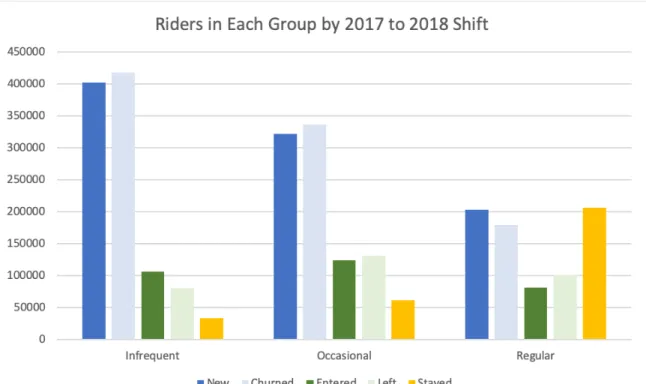
Establishing a fixed definition for these behavioral clusters across years allowed us to use them as a basis for comparing the distribution of behaviors between the two time frames. Investigating which clusters grew in number and which clusters decreased in size gave us insights into the behavioral dynamics behind the overall drop in trips that occurred on the system from the fall of 2017 to the fall of 2018. It also allowed us to identify the cards that churned from the system after 2017, the cards that entered the system in 2018, the cards that were present in both years but exhibited changing behavior, and the cards that exhibited consistent behavior in both years.

In this chapter, we performed the clustering algorithm on all of the cards in the system (except the free cards mentioned earlier). Because of the relatively small number of features and output clusters, this process was not time-intensive (taking fewer than 10 minutes). An alternative method, however, is to cluster several smaller random samples from each year, determine the inter- and intra-year stability, assign fixed centroids based on some combination of the random samples, and then assign each card from the entire set to a cluster determined by the centroid to which it is nearest. Depending on the extent to which stability can be assumed or proven, this method would likely be the most expedient for transit agencies looking to implement this analysis, as assigning each card to the nearest centroid can be accomplished in seconds.

3.4 Results

In the end, we clustered 1,698,851 accounts that were active in 2017 and 1,692,086 accounts that were active in 2018 (including those that were also present in 2017). This section begins with a description of the 2017 clusters themselves and moves on to discuss findings from the longitudinal comparison.

Behavioral dynamics of public transit ridership in Chicago and impacts of COVID-19

Behavioral Dynamics of Public Transit Ridership in

Chicago and Impacts of COVID-19

by

Mary Rose Fissinger

B.S., Boston College (2015)

M.S., University of California, Berkeley (2016)

Submitted to the Department of Civil and Environmental Engineering

in partial fulfillment of the requirements for the degree of

Master of Science in Transportation

at the

MASSACHUSETTS INSTITUTE OF TECHNOLOGY

September 2020

c

○ Massachusetts Institute of Technology 2020. All rights reserved.

Author . . . .

Department of Civil and Environmental Engineering

August 17, 2020

Certified by . . . .

Jinhua Zhao

Associate Professor

Thesis Supervisor

Certified by . . . .

John Attanucci

Research Associate

Thesis Supervisor

Accepted by . . . .

Colette L. Heald

Professor of Civil and Environmental Engineering

Chair, Graduate Program Committee

Behavioral Dynamics of Public Transit Ridership in Chicago

and Impacts of COVID-19

by

Mary Rose Fissinger

Abstract

Acknowledgments

Contents

List of Figures

List of Tables

Chapter 1

Introduction

1.1

Background

1.2

Motivation

1.3

Research Aims

1.4

Data and Methods

1.5

Organization of Thesis

Chapter 2

Background

2.1

How Americans Use Public Transit

2.2

Chicago and the CTA

2.3

The COVID-19 Pandemic

Chapter 3

Customer Segmentation Framework

3.1

Background

3.2

Data

3.3

Methods

3.3.1

K-Means Clustering

3.3.2

Input Feature Selection

3.3.3

Segmentation

3.3.4

Establishing Stability

3.3.5

Longitudinal Comparison

3.4

Results