Design and fabrication of the MesoMill : a five-axis milling machine for meso-scaled parts

(1)

Design and Fabrication

of the MesoMill: A Five-Axis Milling Machine for Meso-Scaled parts

by

Jaime Brooke Werkmeister B. S. Mechanical Engineering University of California, San Diego, 2001

SUBMITTED TO THE DEPARTMENT OF MECHANICAL ENGINEERING IN PARTIAL FULFILLMENT OF THE REQUIREMENTS FOR THE DEGREE OF

MASTER OF SCIENCE IN MECHANICAL ENGINEERING AT THE

MASSACHUSETTS INSTITUTE OF TECHNOLOGY C

May 2004

MASSACHUSETTS INS1MTIUE OF TECHNOLOGY

JUL 2

0 2004

LIBRARIES

I I A / I Signature of Author...--- . . ---1-- . .- -. ...----... . ...

Department of Mechanical Engineering May 7, 2004 Certified by...

.. ... .. .. . ... ...

inder H. Slocum ical Engineering esis Supervisor A ccep ted b y ... ... Ain Sonin am1 cal Engineering Chairman, Committee for Graduate Students

(2)

(3)

Design and Fabrication of the MesoMill: A Five-Axis Milling Machine

for Meso-Scaled parts

by

Jaime Brooke Werkmeister

Submitted to the Department of Mechanical Engineering on May 7, 2004 in Partial Fulfillment of the Requirements for the Degree of Master of Science in

Mechanical Engineering

Abstract

With the increased prevalence of meso-scaled products, new tools are being developed to bridge the gap between fabrication processes tailored for micrometer and millimeter sized features. Compared to its traditional counterpart, a small machine tool designed for meso-scale could potentially have a smaller overall footprint, shorter structural loop and lower cost than a conventional machine; in addition, a small machine presents opportunities for improved machine metrology, and easier environmental control. This paper describes the design of the MesoMill: a test machine designed to evaluate the use of components new to the design of machining centers including wire capstan drives, ball-screw splines, and an air bearing spindle with an integral Z-axis.

Thesis Supervisor: Alexander H. Slocum

(4)

(5)

Acknowledgements

The fabrication of the Mesomill would have not been possible without the aid of Wojciech Kosmowski and Mark Kosmowski of ESI who donated the Westwind aerostatic spindle. Kevan Perkins at THK donated the ball-screw spline. Thomas Massie of SensAble Technologies donated a capstan drive for initial experiments. Sava Industries donated the steel cable for the capstan drive and Alkan Donmez and Brad Damazo of NIST offered their endless knowledge and support in seeing the Mesomill built and tested.

I extend thanks to Mike Roberts who worked on experimentation for the beam bending calculations, Margaret Cho for building the capstan experimental setup, and Brian LaCrosse and Pierece Hayward for helping with the cable testing in the InstronTM machine.

A big thank you also extends to my family and friends. As always my Mom and Dad have been very supporting and encouraging through these few years and through the distant past. Thank you for your encouraging words and long venting hours on the phone. I'm glad the west coast is 3 hours behind the East. By the time I go to bed it's still a decent hour to call and by the time I get up my dad is up going to work. My labmates have been supportive as well. They gave me the right advice at the right time and endless laughs. Special thanks goes to Patrick Willoughby for throwing ketchup packets at me when I slacked off and lending an ear when I needed advise.

Most of all thank you Alex Slocum. He has served as an advisor and friend. He has given me strength and courage in conquering the battle of writing (by the way I still owe him a red pen.) Alex has given me good advice and is a great source of enthusiasm about engineering. I am looking forward to doing my Phud with him.

(6)

(7)

1 Introduction

The objective of this thesis is to present the design of the MesoMill: a five-axis milling machine with intersecting sets of modular axes for the machining of meso-scaled parts. Detailed calculations of choosing and sizing the components of the MesoMill will be discussed.

With the increased prevalence of meso-scaled products, new tools are being developed to bridge the gap between fabrication processes tailored for micrometer and millimeter sized features [1][ 2]. Compared to its traditional counterpart [3], a small machine tool designed for meso-scale could potentially have a smaller overall footprint, shorter structural loop and lower cost than a conventional machine; in addition, a small machine presents opportunities for improved machine metrology, and easier environmental control. This thesis describes the design of the MesoMill: a test machine designed to evaluate the use of components new to the design of machining centers including wire capstan drives, ball-screw splines, and an air bearing spindle with an integral Z-axis.

1.1 Currently Available Machines

Compared to its traditional counterpart, a small machine tool designed for meso-scale parts has the advantages of: ease-of-use, smaller footprint, smaller structural loop, shorter distances between the work piece and the machine's metrology devices, opportunities for improved machine metrology, and easier environmental control [4][5].

There are many machines that can mill small parts, small as in no larger than a 25 mm cube. For instance the 2000/2010 mill by Sherline Products [6]. The overall size of this machine is 381 x 565 x 568 mm and has a tolerance of 10-12 microns. Another machine is the Prazi BF400-450 Powermill Series Precision Benchtop Milling Machine [7] with an accuracy of 5 microns. Its dimensions are 585 x 559 x 813 mm. Similarly, one other machine that produces small parts is the Star Machine by Small Engineering [8]. They specialize in small parts and obtain tolerance of ±5microns, but they use a large machine, roughly 2 x 1.5 x 1 m, to fabricate small parts.

The Modela, model number MDX15 and MDX20, [9][10] is capable of milling and scanning, and is designed for 3D modeling, however given the broad range of tools and accessories available, the Modela can do light machining and PCB manufacturing. The dimensions of the Modela's MDX-15E are 426 x 280 x 305 mm and has a scanning resolution of 50 microns. Another machine, the HexVantageTM _{by Pathfinders} Incorporated [11], can machine in 5 axes and obtain resolution of 0.2 microns per count of its encoder and has an accuracy of 12 microns. This version of a Hexapod can fit on the bench top with dimensions of 1.2 x 1.2 x 1.2 m [12]. Light Machines' BenchmanTM small machining centers are designed to be placed on top of a bench, and operate with high speed spindles for CNC machining of small parts with features as small as 10-20 microns [13].

(10)

Sandia National Laboratories in their Manufacturing Science and Technology Center [14], have began to develop four new meso-machining technologies which are: Focused ion beam (FIB) machining, Micro-milling and -turning, Excimer and Femto-second laser, and Micro-Electro Discharge Machining (Micro-EDM) [15]. These meso-machines will create features sizes in the micron range between 1-50 microns. The Micro-wire EDM has a positional accuracy of ±1.5 microns and the Femto-second laser machining can machine a hole with a micron in diameter.

Researchers have also been investigating new approaches to machine and process design for manufacture of small parts. For example, DeVor and Kapoor at the University of Illinois [16] have been working on the "Development of a Meso-Machine Tool System" [17], and indications are that it is indeed worthwhile to investigate configurations for meso machines that are not merely scaled-down versions of macro machines.

1.2 Characteristics of the MesoMill

When considering the manufacture of small parts, one design option not regularly used in large machines, due to size issues, is collinearity of axes. Given this design, a logical question that was sought to be answered was can a ball-screw spline shaft, which can provide linear and rotary motions, be oversized so it could also serve as the principal moving structural element? It is this concept that was chosen for consideration. A MesoMill which uses this concept is shown in Figure 1. It is designed to be a 5-axis milling machine that is capable of machining components no larger than a 25 mm cube and it has a size of about 400 x 400 x 400 mm. A five-axis machine allows for five sides of a part to be machined in one setup, thus minimizing errors introduced by re-clamping

[18].

The fundamental design principle of the Mesomill is to use two intersecting linear/rotary axes which support the workpiece and a Z-0 spindle assembly, respectively. The air bearing spindle, from an ESI circuit board drilling machine, has a speed range of 40,000 to 110,000 rpm, and the spindle incorporates a linear machining axis in Z with a travel of 10 mm. The other four machining axes are realized by two identical orthogonal THK1 ball-screw splines, each producing a combination of linear and rotary movement. Wire capstan drives couple the servo motors to the ball-screw spline. This design has the advantage of no backlash and a high rotational stiffness on the order of 6,000 N-m/rad. Positioning feedback is achieved close to the workpiece using a new encoder capable of simultaneously measuring both linear and rotary movement. An error budget of the machine was developed, and used to help determine the proper placement of the nuts on the ball-screw spline shafts to give an "optimal" spacing to reduce errors.

Commercial equipment, instruments, or materials are identified in this thesis in order to specify adequately certain procedures. In no case, does such identification imply recommendation or endorsement by the author, nor does it imply that the material or equipment identified is necessarily the best available for

(11)

Capstan Drive Motor THK Ball screw-spline Aerostatic 49 Spindle

Figure 1: MesoMill prototype (left) and solid model (right)

(12)

2 Background

The hypotheses that a small machine can best be used to make small parts, 6 functional requirements were established:

1. Move in 5 axis

2. Part size of 1 inch cube or less 3. Accuracy on the order of 1 pm 4. Stiffness of machine about 50 N/ pm 5. Desktop machine, 800 mm cube and 6. Cutting material is steel

The original version proposed by Professor Slocum, had two axis crossed as in Figure 2. After building a wooden model of this configuration, it was noticed if the axis were at right angles to each other a wider range of machining capability would be produced. This created the first concept for the MesoMill.

Figure 2: Preliminary concept of the MesoMill presented by Professor Slocum

The main concern having a machine this small is its stiffness and damping characteristics. A small machine that has insufficient stiffness and cannot damp the vibrations from the cutting force is inadequate compared to the standard precision CNC machines234. To overcome these features, the ball screw spline shaft by THK [19] was looked upon, along with air bearings by New Way Bearings5 to control the chatter from the aerostatic spindle which was donated by ESI6.

2 _{Bob6 Services Group, Inc. Esslingen, Germany, 1996. http://www.boko.com/}

3 Mecona Teknik AB, Keckel Maho DMU 50 eVolution, 2002. http://www.mecona.se/dmu50ev.htm

4 Makino, 5-axis machining center, 2000. http://www.makino.co.jp/product e/

5 NewWay Bearing, http://newwaybearings.com/productpages/airbushings.html 6 _{ESI Corporation, http://www.esi.com/}

(13)

Analysis was performed on the MesoMill. These include: error analysis, tool stiffness, beam bending, natural frequency of the system, and motor determination (capstan drive, dual pinion, iterative process to figure out proper motor.) The analysis will be discussed in more detail in chapter 4.

Secondly, experiments were performed to confirm analytic results, and gather data where calculations could not be performed. The experiments include: bending the shaft under a given force, stiffness of air bearings, torsional stiffness of a capstan drive, and errors in an aerostatic spindle. The experiments and results are shown in Chapter 5.

In Chapter 6, suggestion will be given and then the conclusion will follow to put everything in perspective. References are listed at the end but before the Appendix. The appendix contains evolutionary pictures of the MesoMill, data, and further details of the calculations.

(14)

3 Preliminary Concepts of the MesoMill

Presented below are the preliminary design concepts updated as more analysis was performed.

Initial concept of the MesoMill which was originally Note the axes are crossed.

of the MesoMill. Each version was

presented by Professor Slocum.

Cb

Figure 3: Concept 1 of MesoMill by Professor Slocum.

Sketch to see if possible to machine in all 5 axis and if the axis could be perpendicular (right angle) to each other instead of crossed. It was shown the right angle axes can machine efficently compared to the crossed. More components were needed if the axes were crossed as in Figure 3.

Figure 4: Determination if can machine on all 5-axis.

Bench level experiment of the solid model in Figure 4 is given in Figure 5. This experiment was to see if the right angle axis would be able to machine in all 5 axes.

(15)

Figure 5: Bench level experiment of machining capability of MesoMill.

Solidworks representation of what the MesoMill could look like. Since this is an early drawing, all the components were still being sized.

Figure 6: Preliminary sketch model of MesoMill

Bench level Experiment of how the right angle axis would move in relation to the other axis.

(16)

Below is the overall configuration of the MesoMill with the two axes, spindle and work piece at right angles to each other. The large cylinders are the motors that drive the ballscrew-spline nuts and the rectangles are where the air bearings would reside.

Figure 8: Configuration of axis.

The spindle axis will be mounted in a V-groove. This shows how the spindle will move. The long rectangle on top is the motor. In subsequent chapters it will be shown the V-groove is not necessary.

U,

Figure 9: Preliminary mounting of ballscrew-spline in holder

Side view of the V-groove and spindle axis. The rectangle in the back represents where the motors are placed.

(17)

Figure 10: Side view of v-groove mounting.

Isometric view of what the spindle axis will look like. How the shaft will be attached is shown by the copper color plates.

Figure 11: Overall view of v-groove mounting of spindle axis.

Drawing of the experiment apparatus. The goal was to see how much the tip deflects if a force is implemented between the ball screw-spline shaft (by THK.)

Air bearing sleeves 0 @0 -

~

. ...

(18)

Figure 12: Model of the experimental setup of ball screw-spline

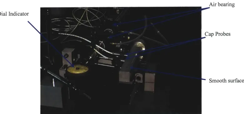
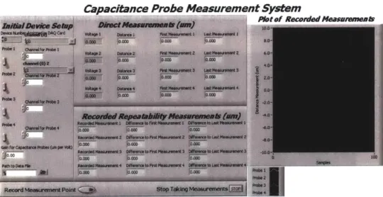
Linear bearings with a shaft through them. Steel blocks on the side hold the capacitance probes. These devices send out a voltage when movement is detected.

Figure 13: Bearing block experimentation setup.

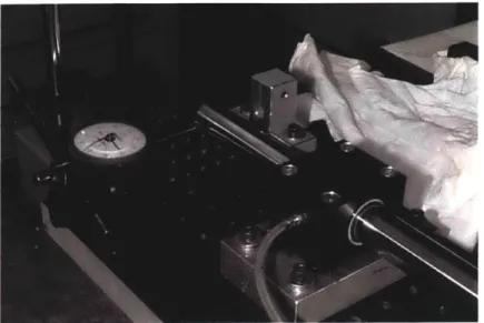
Long view of what the shaft and linear bearings looked like.

(19)

Figure 14: Long view of bearing block experimentation.

Top view of the input force onto the shaft and the detection of movement by the

capacitance probe (bottom left of picture.) Square block on the shaft was used in aligning and detecting movement of the shaft.

Figure 15: Top view of bearing block experimentation. For the results of these experimentations refer to Chapter 6.

(20)

Lastly the final concept for the MesoMill is shown below. Motor Casta _{THK Ball} screw-spline SS Aerostatic Spindle

(21)

4 Calculations

There were many calculations performed to determine the feasibility of the MesoMill. Calculations performed on the ball screw-spline shaft were: error analysis, tool stiffness, beam bending, natural frequency, V-block hertz contact/top plate bending, and motor siz-ing. The calculations performed to compare two options for the transmission were a cable capstan drive and dual pinion. Each calculation is described below and the results are presented in the results section.

4.1 Error Analysis

An error budget of the MesoMill was created to compare it to a normal size machine which assesses whether the concept has merit. The MesoMill can be divided into two primary components, the work and tool path, which each are attached to a comparatively rigid base, as shown in Figure 1. In Figure 17 the structural loop of the work and tool path is shown. The total distance from the reference base to D5 is considered the work

path where: D1 is the distance from the reference to the midsection between the two nuts on the ball-screw spline, D2 is the distance from the midpoint of the nuts to the end of the ball-screw spline shaft where the disc connects, D3 is the distance from the end of the

shaft through the thickness of the disc, D4 is the distance from the disc to the fixture, and

D5 is the distance from the fixture to the part. The total distance from D6 through D12 is considered the tool path where: D6 is the distance from the tool tip to the collet, D7 is the distance from the collet to the center of the shaft in the air bearing spindle which gives the spindle translation, D8 is the distance from the shaft center to the air bearings in the

aerostatic spindle, D9 is the distance from the air bearings to the spindle holder mount,

DIO is the distance from the holder to its connection on the ball-screw spline shaft, DI1 is

the distance from the end of the shaft to the midpoint of the ball-screw spline nuts, and D12is the distance from the midpoint of these nuts to the reference base.

(22)

z

Z

Y

d

X

Ballscre v nuts

Figure 17: Structural Loop, shown in red, of the MesoMill: Work path is from the work piece to the center of the nuts (D1-D5). The tool path is from tip of tool to the center of

the nuts (D5-D12).

Given the right angle configuration shown in Figure 17, Table 1, and Table 2 show the estimated errors for each distance DI - D5 for the work path and D5 - D12 for the tool path. For these estimates, the individual component-to-component alignment errors are

estimated to be 10 ppm. Misalignment of the tool extension in the chuck and through the shaft in the aerostatic spindle is the largest contributing factor to the error. The further the Z-axis (D8 increases) of the spindle is extended, the larger the error. With the Z-axis retracted and the axes centered, the predicted accuracy is 8 microns. With all the axes at the limit of their travel, the predicted accuracy is 9 microns. By mapping of the axes' errors, a factor of 10 improvement is expected because there are only preloaded rolling element joints in the machine. A setting tool station can also be used to reduce all offsets [20]. SD3 D4 D D5 D1 Ballspline nuts Reference base D12

(23)

Table 1: Work path error for retracted and extended tool. The relative dimensions of each coordinate system are given along with its random errors. Random errors are predicted to be 10 ppm of length of component.

Retracted Part-to-Fixture (D5) Fixture to Disc (D4) Disc to Shaft (D3)

Dimensions Random Dimensions Random Dimensions Random

(mm) Errors (mm) Errors (mm) Errors

Axes (pm) (pm) (pm)

X 0.0 0.25 0.0 0.13 0.0 0.32

Y 0.0 0.25 0.0 0.13 0.0 0.32

Z -25.4 0.25 -12.7 0.13 -12.7 0.32

OX (rad) 0.0 1.OE-5 0.0 1.OE-5 0.0 1.OE-5

OY (rad) 0.0 1.OE-5 0.0 1.OE-5 0.0 1.OE-5

OZ (rad) 0.0 1.0E-5 0.0 1.OE-5 0.0 1.OE-5

Retracted Shaft to Bearing (D2) Bearing to Reference (D1)

Dimensions Random Dimensions Random

(mm) Errors (mm) Errors

Axes (pm) (pm)

X 0.0 1.68 -240.0 2.4

Y 0.0 1.68 0.0 2.4

Z -125.7 1.68 0.0 2.4

OX (rad) 0.0 1.OE-5 0.0 1.OE-5

OY (rad) 0.0 1.OE-5 0.0 1.OE-5

OZ (rad) 0.0 1.OE-5 0.0 1.OE-5

Sum Random Errors RSS Random Errors Average SUM & RSS random

in the reference CS in the reference CS errors in the reference CS

8X (j m)= 7.7 8X (pm)= 4.8 8X (pm) = 6.2

8Y ( m) = 7.7 6Y (pm)= 4.8 8Y (pm) = 6.2

5Z (pm)= 4.8 5Z (pm)= 2.9 8Z (pm)= 3.9

eX (rad) = 50.0 sX (rad) = 22.4 sX (rad)= 36.2

sY (rad) = 50.0 sY (rad) = 22.4 sY (rad) = 36.2 sZ (rad) = 50.0 sZ (rad) = 22.4 sZ (rad) = 36.2

(24)

Extended Part-to-fixture (D) Fixture to Disc (D4) Disc to Shaft (D3)

(mm) Errors (mm) Errors (mm) Errors

Axes (pm) (pm) (gm)

X 0.0 0.25 0.0 0.13 0.0 0.32

Y 0.0 0.25 0.0 0.13 0.0 0.32

Z -25.4 0.25 -12.7 0.13 -12.7 0.32

OX (rad) 0.0 1.OE-5 0.0 1.OE-5 0.0 1.OE-5

OY (rad) 0.0 1.OE-5 0.0 1.0E-5 0.0 1.OE-5

OZ (rad) 0.0 1.OE-5 0.0 1.OE-5 0.0 1.0E-5

Sh6 l + B k D n B t f-)

Extended (D1)

Dimensions Random Dimensions Random

(mm) Errors (mm) Errors

Axes (pm) (pm)

X 0.0 1.68 -240.0 2.4

Y 0.0 1.68 0.0 2.4

Z -176.5 1.68 0.0 2.4

OX (rad) 0.0 1.OE-5 0.0 1.OE-5

OY (rad) 0.0 1.OE-5 0.0 1.OE-5

OZ (rad) 0.0 1.OE-5 0.0 1.OE-5

5X (pm)= 8.4 8X (m) = 5.2 8X (gm)= 6.8

8Y (m) = 8.4 8Y (pm) = 5.2 5Y (tm) = 6.8

8Z (m)= 4.9 5Z (pm)= 2.9 8Z (pm)= 3.9

eX (rad) = 50.0 sX (rad) = 22.4 sX (rad)= 36.2 &Y (rad) = 50.0 sY (rad) = 22.4 &Y (rad)= 36.2 sZ (rad) = 50.0 sZ (rad) = 22.4 sZ (rad)= 36.2

. ... ...

(25)

Table 2: Tool path error for tool retracted and extended. The relative dimensions of each coordinate system are given along with its random errors.

estimated to be 10 ppm of component length.

Each random error is

Retracted Tool tip to Collet (D6) Collet to Shaft (D7) Shaft to Bearing (D8)

Dimensions Random Dimensions Random Dimension Random

(mm) Errors (mm) Errors s (mm) Errors (pm)

Axes (p1n) (9m)

X 0.0 0.1 0.0 2.5E-3 0.0 2.5E-3

Y 0.0 0.1 0.0 2.5E-3 0.0 2.5E-3

Z -44.4 0.0 -60.2 0.0 12.7 0.0

OX (rad) 0.0 1.OE-5 0.0 1.OE-5 0.0 1.OE-5

OY (rad) 0.0 1.OE-5 0.0 1.OE-5 0.0 1.OE-5

OZ (rad) 0.0 1.OE-5 0.0 1.OE-5 0.0 1.OE-5

Retracted Bearings to holder (D9) Holder to Shaft (DIO) Shaft to Bearings (D1 I)

Dimensions Random Dimensions Random Dimension Random

(mm) Errors (mm) Errors s (mm) Errors (pm)

Axes (pm) (pm)

X 0.0 0.9 50.8 0.25 189.2 189.2

Y 0.0 0.9 0.0 0.25 0.0 0.0

Z -39.5 0.0 -131.4 0.25 0.0 0.0

OX (rad) 0.0 1.OE-6 0.0 1.OE-5 0.0 0.0

OY (rad) 0.0 1.OE-6 0.0 1.OE-5 0.0 0.0

OZ (rad) 0.0 1.OE-6 0.0 1.OE-5 0.0 0.0

Retracted Bearings to Reference (D12) Dimensions Random (mm) Errors Axes (pm) X 0.0 2.7 Y 0.0 2.7 Z 227.4 2.7 OX (rad) 0.0 L.OE-5 OY (rad) 0.0 1.OE-5 OZ (rad) 0.0 1.OE-5

8X (Gm) = 8.1 8X (tm) = 3.6 8X ( tm) = 5.8

8Y (pm)= 11.0 8Y (gm)= 5.6 8Y (gm) = 8.3

8Z (pm)= 7.1 8Z (gm)= 5.2 8Z (pm)= 6.1

PX (rad) = 60.1 &X (rad) = 24.5 sX (rad) = 42.7

cY (rad) = 60.1 eY (rad) = 24.5 sY (rad) = 42.7

sZ (rad) = 60.1 sZ (rad)= 24.5 sZ (rad) = 42.7

... . .

, E ... - - -4WilgM

(26)

Extended Tool tip to Collet (D) Collet to Shaft (D7) Shaft to Bearing (D8)

Dimensions Random Dimensions Random Dimensions Random

Axes (mm) Errors (pm) (mm) Errors (pm) (mm) Errors (pm)

X 0.0 0.1 0.0 2.5E-3 0.0 2.5E-3

y 0.0 0.1 0.0 2.5E-3 0.0 2.5E-3

Z -44.4 0.0 -60.2 0.0 12.7 0.0

OX (rad) 0.0 1.OE-5 0.0 1.OE-5 0.0 1.OE-5

OY (rad) 0.0 1.OE-5 0.0 1.OE-5 0.0 1.OE-5

OZ (rad) 0.0 1.OE-5 0.0 1.OE-5 0.0 1.OE-5

Extended Bearings to holder (D9) Holder to Shaft (DI0) Shaft to Bearin gs (D1 )

Axes (mm) Errors (pm) (mm) Errors (ptm) (mm) Errors (pm)

X 0.0 0.9 50.8 0.25 189.2 1.68

Y 0.0 0.9 0.0 0.25 0.0 1.68

Z -64.9 0.0 -131.4 0.25 0.0 1.68

OX (rad) 0.0 1.OE-6 0.0 1.OE-5 0.0 1.OE-5

OY (rad) 0.0 1.OE-6 0.0 1.OE-5 0.0 1.OE-5

OZ (rad) 0.0 1.OE-6 0.0 1.OE-5 0.0 1.OE-5

Extended Bearings to Reference (D12) Dimensions Random Axes (mm) Errors (ptm) X 0.0 2.7 Y 0.0 2.7 Z 227.4 2.7 OX (rad) 0.0 1.OE-5 OY (rad) 0.0 1.OE-5 OZ (rad) 0.0 1.OE-5

6X m m= 9.7 5X (pm)= 4.3 8X (pm)= 7.0

1Y

(pm) = 2.6 8Y (gm)= 6.4 8Y (pm)= 9.5

5Z (pm) 7.1 5Z (pm)= 5.2 8Z (pm)= 6.1

sX (rad)= 60.1 gX (rad) = 24.5 sX (rad) = 42.7

sY (rad)= 60.1 sY (rad) = 24.5 sY (rad) = 42.7

sZ (rad)= 60.1 sZ (rad) = 24.5 sZ (rad) = 42.7

The largest estimated random error is 2.7 microns from the bearings to the reference base due to the distance from the axis to the center of the bearings. This is the same reasoning for the work path error for a value of 2.4 microns.

As seen from Table 2, the major two errors are from the bearing to reference and the tip of the tool to the collet. In order to reduce these errors the structural loop would have to be decreased. Minimal amount of the tool shank should be exposed out of the collet. As for the bearing to reference, the retracted position would be most beneficial to cut at. No design alteration at this point for the distance between the bearings to the reference can be made.

(27)

Now if the spindle is moved in the y-direction, Table 3 and Table 4 are produced, note the work path can not change in the y direction, only the tool path can. These tables show that the error is the same but the movement has changed from the z-axis to the y-axis.

Table 3: Work path with movement in x and y directions. No movement in y can be performed within the work path. Note the random error values and dimensions of the coordinate systems are in Appendix B. Each random error is estimated to be 10 ppm of length of component.

8X (Im) = 7.9 8X (pm) = 4.7 8X (pm)= 6.3

6Y (pm) = 7.8 6Y (9m) = 4.7 8Y (pLm)= 6.3

8Z (_m)_ = 4.9 8Z ([m)= 2.9 8Z (pm)= 3.9

sX (rad) = 50.0 sX (rad) = 22.3 sX (rad)= 36.2 sY (rad) = 50.0 eY (rad) = 22.3 EY (rad) = 36.2

sZ (rad) = 50.0 sZ (rad) = 22.3 &Z (rad)= 36.2

Table 4: Tool path with movement in the x and y directions. Note the random error values and dimensions of the coordinate systems are in Appendix B. Each random error is estimated to be 10 ppm of length of component.

8X (Rm) = 8.1 8X (pm) = 3.6 8X (pm) = 5.8 8Y (pm) = 8.1 8Y (pim) = 5.2 8Y (pm) = 6.7 8Z (jm) = 10.0 8Z (pLm) = 5.5 8Z (pim) = 7.8 sX (rad) = 61.0 &X (rad) = 24.5 sX (rad) = 42.8 sY (rad) = 61.0 sY (rad) = 24.5 sY (rad) = 42.8 sZ (rad) = 61.0 sZ (rad) = 24.5 eZ (rad)= 42.8

The error for the tool and work path for the above case is 7 microns. Note the largest errors are in the 8Y direction for the tool path and 8Y and 8X direction for the work path. Thus the errors are better handled with the movement in the X and Y direction and should be used while machining.

Now with movement in the y and z directions, Table 5 shows the new configuration and errors. The work path has the same values as Table 3.

.1 ... 1"" "' "" "' " .. .. .

(28)

Table 5: previous. Appendix

Tool path movement in the x, y, and z axes. Work path is same case as Note the random error values and dimensions of the coordinate systems are in B. Each random error is estimated to be 10 ppm of length of component.

8X (m)= 10.7 5X (gm) = 5.2 5X (pm) = 7.9

8Y (pm)= 10.0 8Y (pm) = 6.5 8Y (pm) = 8.20

5Z (m)= 10.8 8Z (pjm) = 6.0 5Z (pm)= 8.4

sX (rad) = 61.0 sX (rad) = 24.5 eX (rad) = 42.8 sY (rad) = 61.0 sY (rad) = 24.5 sY (rad) = 42.8 sZ (rad) = 61.0 sZ (rad) = 24.5 sZ (rad)= 42.

The tool path error is 8 microns and the largest occurs in the 6Y direction. Again as stated above, a factor of 5-10 times improvement of the axes' errors is expected because there are only preloaded rolling element joints in the machine.

The above tables show the machine's accuracy is determined by two important distances, bearings to reference point and tool tip to collet. These can be reduced by machining in the x and y directions and keeping the distance small.

4.2 Tool Stiffness

The stiffness of the tool was used in the error analysis calculation to determine how much the tool bit would deflect given the cutting force. To calculate the stiffness of a standard tool requires knowing the elastic modulus, diameter, and length of the tool. The deflection for a tool, which is in any standard strength of materials book [21], is

=5 PLE

3EI

(1)

Rearranging the above equation to give the stiffness K:

P 3EI

The polar moment if inertia I is

IP = ;d

" 32

(2)

and substituting this into the equation for stiffness gives the strength of the tool in terms of modulus of elasticity, diameter of the bit, and the length of the tool:

3gd4

K = 3L

32LP

(29)

(3)

Since a tool bit has two diameters, DI for the shaft portion and d2 for the cutting portion,

the stiffness of each section is calculated and then added like springs in series to give the over all stiffness of

1 1 1

Ktot KD1 Kd2

(4)

Assuming the tool is steel makes the modulus of elasticity 2.1 N/mm2 _{and taking a}

stan-dard tool of D1 3.175 mm with length of 12 mm and d2 0.5 mm with length of 0.5 mm

makes the stiffness 3254 N/mm

4.3 Beam Bending

The principal moving structural elements are the ball-screw splines, and originally it was thought that the ball-screw splines could project through air bearing sleeves in order to provide a greater degree of accuracy and dynamic stiffness, refer to Figure 10. In the next subsection and in Chapter 6 it is shown this is not the case. The grooved portion of the shaft could be of a smaller diameter than the portion through the air bearings, and hence radial error motions induced by the nuts could be reduced. Figure 18 shows the model of this concept [22]. It is found, as the length of c and d increase, the deflection ratio between the work piece end (x = 0) and the nut end (x = c + d) decrease for a given radial deflection at the nut; however, the size of the machine grows in proportion to its workspace. This poses the question, how much "self coupling" is desired verses buying more accurate components in the first place?.

Y C d D D2 KA _K b FA F M F1 x

Figure 18: Stepped shaft model of the ball-screw spline supported at its front end by air bearings, where radial displacement from the nut closest to the air bearings is applied to the end of shaft segment D2.

However, adding length to the shaft to enable it to be supported by the air bearings makes the machine very large with respect to its work volume; hence an important part of the tests are to determine if they are really even needed. Thus the initial test machine does

. .. ...

(30)

not use the air bearings to help support the shaft; it only uses the screw and ballspline nuts. This is one of the fundamental principals in deciding to use the nuts on the ball-screw spline to support the shaft because it is compact and no additional component are needed to increase the accuracy. The next section describes the beam theory for two types of beams, a constant diameter and a variable diameter shaft. Then the proper sizing of the shaft is presented for each case.

4.3.1 Beam theory background

The ball screw-spline with two air bearings supporting the far end of the shaft can be represented as a beam with two springs. Figure 19 describes what the system should look

like.

Figure 19: Shaft diameter shaft with 2 air bearings

When a force is applied between the center of the ball screw-spline nut, it is necessary to determine the deflection in the beam, namely at the opposite end of where the force is applied, Figure 20. Y C D1 F Ka Kb a| b Figure 20: Forces on a beam.

Assuming the beam has constant flexural rigidity, EI where E is the modulus of elasticity and I is the moment of inertia, the deflection of the beam can be determined. If the beam did not have constant flexural rigidity, EI would be a function of x (See the section on variable cross section below.) Thus by assuming constant flexural rigidity, the

(31)

calculation is more desirable. To determine the deflection of the beam, the equation for the elastic curve is found. The equations to obtain the elastic curve are:

EI = -q(x) (5) EI V(x)= - _{Jq(x)dx+ C,} (6) EId = M(x)=-- dx

Jq(x)dx

+ Cx +C2 dix2 (7) EId = EIO(x)= =dx dx q(x)dx +1CIx2 +C2x _{+ C}

dx 23

EIy(x) = --

r

fddx d (x) dx + C ₆ + ₂Cx C2X2 + C3x + C4

(8)

(9) These equations are derived in any mechanics of materials book [21]. Noticing four constants of integration, these values can be obtained from the boundary conditions of the

system. The boundary conditions of the beam/spring system are:

V(0) = 0 (10) M(0) = 0 (11) y(a) =81 (12) y(b) =82 (13) The first two conditions are obtained from the shear and moment forces at the ends of the beam. Since there are no shear or bending moment at the ends, the values are 0. The last two conditions are obtained from the beam supports. The value of deflection or the value ofy at the supports is equal to the amount of deformation that the individual supports go through. Since they are modeled as springs, the deflection is 5 =F/K.

(32)

To determine q(x), the concept of singularity functions will be used. Singularity functions have the form

f

(x) = (x - a)"

(14) This is valid for n 0. For 0 n

f,

becomes 0 because the expression in the brackets is negative. If the expression is positive, then the value of

f,

is (x-a)". Notice the brackets changed to parentheses or ordinary brackets when the quantity inside is positive. Likely when 0 n,

f,

is 0 no matter what the value is in the brackets. The singularity function has the following integration law

(x - a)"dx = (x - where n 0

n +1

(15) The value of n represents the different loading types. For example when n = -2, this represents a unit concentrated moment. Similarly when n = -1,0,1, this represents a unit concentrated load, unit step, and unit ramp respectfully. The loads on the system presented in Figure 20, which are the air bearings, are represented as concentrated loads.

Lastly for cases of n= -2 and -1, the values are 0 everywhere except at x=a. At that point they are infinite. They are included in the calculations but n is written as a subscript instead of a superscript because in (15) n 0. Upon integration, they become <x-a>-2 =

<x-a>.1 and <x-a>1 = <x-a>0.

4.3.2 Beam Analysis - Constant shaft deflection

(33)

Y C D1 F Ka Kb b Fa Fb F x

Figure 21: Free body diagram of a constant diameter beam.

Summing the forces in the y direction with up as positive and assuming the forces are all pointing up for ease of calculation, gives the following equation

F =O=F +FB +F

(16)

Solving for FB

B -F-F

(17) Summing the moments around the spring B:

IMB =0 =-(b -a)F +(c -b)F

(18) Solving for F, results in

F =Fc-b_b-a

Notice how the value of the angle was not needed because it cancels out. value of FBin terms ofF , sub (19) into (17) to get

(19) To get the

(34)

(20) Factoring out F, FB becomes

=-F c -a

b-a

(21)

Elastic Equation

Since the reaction forces are found, the load is determined next. There are two concentrated loads on the beam, F and FB . Using singularity functions and starting the cut from the left-hand side (Figure 21), the load equation can be represented as:

q(x)= F,(x -a), + FB(x-b) +F(x-c)_

Substituting (22) into (6) gives the shear for V(x):

(22)

V(x) = -(F (x -a) + FB(x - b)0 + F(x - _{c)) + CI)}

(23) Notice how the power on the singularity function increased by one because of integration.

To find the constant C1, the boundary condition given by (10) will be used. Subbing in 0

for x and 0 for V(x) gives:

C, = 0

C, = 0 (24)

The terms in the brackets are negative, so according to the singularity function they are 0. Also one can not have a negative length. Thus the constant of integration drops out and the shear equation becomes

V(x) = -(F,(x-a) +FB(x -b)0 +F(x-c)0)

(25) Integrating (25) to find the bending moment equation, which is done by substituting (25) into (7) reveals:

F-F c -b -F

(35)

M(x) = FA(x -a)' + FB(x -b) + F(x -c) + C2

(26) But the boundary condition given by (11) states there is no bending moment at the end where x is equal to zero. Plugging in these values produces C2 equal to 0 and (26)

becomes

M(x)= FA(x-a)' + FB(x -b) + F(x -c)'

(27) which is the bending moment equation. The slope of the beam is determined next by substituting (27) into (8): EIO(x) = (x - a)2 2 Leaving C3 in the deflection: F a) EI(x)= ^(x-6a)3 6 FF + ₂B 2( ₂ X-C)2 + C 3 (28) equation and integrating once more to obtain the equation for

FF

+ B

(x

_ b)+ ±-xc) 3 +C3x+C

6 6

(29) To solve for the two constants C3 and C4, we know the deflection at the two supports A

and B. That is, the deflection is equal to the force divided by the spring's stiffness. This is boundary condition (12) and (13). Substituting (12) into (29)

F F F F

EI(- A)= (a-a)3 + (a-b) F (aC)3+Ca+C

K 6 6 6

(30) The first term after the equal sign is 0 because the lengths are the same. For the second term, it is 0 also because the value inside the brackets is negative. From the definition of singularity function described above, a negative value is not recognized so the value is 0. The third term is 0 as well because the value of a-c is negative; the value of a cannot be greater than c. Thus, due to the same reasons for the third term, < a-c>2 _{is 0. Reducing}

(30) and solving for C4

C4 =

-EI

FA +C3aJ

KA

(36)

Going back to (29) and inserting the last boundary condition known, (13), the following equation is obtained F F F F EI(- B _ A a) + fB (-) b - _ (b-c)C + b3±4 KB 6 6 6 (32) The second, third, and fourth terms are 0; lengths cancel out and have negative value in the brackets, respectfully. Angle brackets can be removed and replaced by parentheses because the value of b-a is never negative. The first term is not 0 because the value is

positive. Substituting (31) into (32) produces

EI FB _

KB) F^ (b-a)3+_C(b)-EI 6 K)F^ -Csa

(33)

C3 can be determined by collecting similar terms and dividing by b-a. That is

C3= 1[EI(FA FBA FA(b-a)]

b-a YKA KB) 6

(34)

F1 and F2 are known from (19) and (20). Thus C3 is

C3 = EIrF b+F c-aF c-b(b - a)3

b-a KA b-a KB b-a)6 b-a

Factoring out F and EI, (35) from above:

C3 = b+ I- -61I (b - a)3

b-a KA b-a KB b- a 6EI b-a

(36) The values of F1 and F2can be substituted into C4. This makes (31) become

(35)

C4 = EI- F c-b -C3a

KA b--

(37) Substituting (36) into (37) gives the value of C4

(37)

F c-b _ FEI 1 c-b 1 c-a 1 c -b

C

4 =EIFK--1-

[

-

+

---

(b -a)a

KA b-a _b-a KA b-a KBb-a 6EI b-a

(38) Factoring out F, EI, and a negative sign produces the following

C4 =FIr I c-b a 1 c-b + Ic-a 1 c- (b 3j j

K b-a b-a K b-a KB b-a 6EIb-a

(39) The value of 8(x) can now be determined because the constants are known. Substituting (19), (21), (36), and (39) into (29):

EIS(x)=- F c-b(x -a) F c-a (x-b)3 + (x-c)3+

6b-a 6b-a 6

FEIF 1 c-b 1 c-a 1 c-b 31 +

--- -- -- --- -(b-a) _{1 1}x+ b-a K A b-a K B b-a 6EI b-a

FEI - c-+ a Icb+ 1 -- 1- (b -a)3

K [ b-a b-a KA b-a KBb-a 6E1b-a _

(40) Factoring out F and dividing by the flexural rigidity, the elastic curve equation becomes

1 1 c-b(x-a)₃ _ c-a (x-b 3+ _(x-C) ₊

EI 6b-a 6b-a 6

ra(x)

= Fb[ + c-a 1 c-b(b a)' jx

b-a K b-a KB b-a 6EIb-a

- - +--a [1cb+ I - (b - a)3

K[ b-a b-a KA b-a KBb-a 6EIb-a

(41)

4.3.3 Placement of Components

The goal of the above exercise was to find the proper placement of the ball screw-spline nuts in relation to the air bearings. The point of minimal deflection is desired. To find the correct position of the nuts relative to the air bearings, the ratio of deflection at the force end (when x=O) to the deflection at the end of the beam (when x=c) is compared against the ratio of the length, b/a. The deflection when x equals zero is considered 6(0) and the deflection at the opposite end of the beam is considered 8(c). Taking these values

(38)

and plotting them, will result in a graph that portrays how much a deflection or error will result at the end opposite of where the force is applied.

Before the graph is made, the equation for 8(0) and 6(c) is found by plugging in the values described above into (41). The following two equations are obtained:

J(0)= F[ I -b+ a - + I - -1 b -a)3

KA b-a b-a KA b-a KB b-a 6EIb-a )

(42)

I ( c-b(c-a) _{1c-a (c} _{-b)'+ (c-C)+}

El 6b-a 6b-a 6 )

6(c)=F + c-a - (b-a)3

c+

b-a KAb-a KB b-a 6EIb-a

- c-ba[ 1 c-b + c-a 1 c-b a)

KAb-a b-a K b-a KB b-a 6EI b-a

But (43) can be reduced further because c-c is 0. Therefore (43) becomes

i(c) = F

L1

1cb(c-a)3- Ic-(c _-b)' ₊

1 6b-a 6b--a

1_+ [b I _1 c-a 1 cbb

a+ 1)l

b-a K b-a KB b-a 6EI b- a

- +- a - + c - (b -a)'

KA b-a b-a KA b-a KB b-a 6EI b-a

(43)

(44)

F does not need to be known because it cancels out when the ratio 5(0)/(c) is taken.

(39)

- + a + - (b - a)3

K b-a b-a K b-a KBb-a 6EI b-a

9(c)-

-1 I c-b(c-a)3 _{c-a c-b) +}

EI 6 b- a 6b-a )

b ic-a 1 c-b(ba)jc+

b-a KA b-a KBb-a 6EIb-a

b -b a K b K c-a 6Ib-a (b a)3

KA b-a b-a[KA b-a KBb-a 6EIb-a

Inputting different graph is obtained 0 cc 0 CD (45)

values for b and a and comparing 6(0)/8(c) versus b/a, the following

Deflection Ratio VS. b/a

0.8 0.7 0.6 0.5 0.4 0.3 0.2 0.1 0 -0.1 -0.2 -0.3 - Series1 - Series2 Series3 - Series4 -- Series5 -- Series6 - Series7 -- Series8 -- Series9 Seriesl0 Series 11 Series12 -- Series 13 -- Series 14 0. - eis 0. - eis 0.1 - Se-i-s 2 3 4 5 6 b/a

Figure 22: Deflection Ratio for constant shaft

(40)

Table 6: Length values for c and a are in meters Series c a 1 1.14 0.13 2 1.12 0.13 3 1.09 0.13 4 1.07 0.13 5 1.04 0.13 6 1.02 0.13 7 0.99 0.13 8 0.97 0.13 9 0.94 0.13 10 0.91 0.13 11 0.89 0.13 12 0.86 0.13 13 0.84 0.13 14 0.81 0.13

Notice how the graph originally dips down. Then rises through zero and ends in a steep slope. The steep slope is a result of the air bearing being placed past the overall length c. Naturally the equation would go towards infinity if the placement of the bearing were beyond the shaft length. When the bearings are close together, the deflection ratio starts to increase causing one end of the beam to point in one direction while the other end points in the opposite direction. As the distance between the bearings increase, the deflection comes to a point where it levels off and starts to decrease. This represents the bearings obtaining a certain distance that can hold the shaft in a stable position without it

tilting. As the graph passes through the x-axis, the two ends of the shaft point in the same direction. This implies there is a point of zero deflection. That is the point, which is most desired.

As a is decreased, the point of zero deflection moves towards the right on the graph. Thus the distance between the air bearings is larger than if a started further in on the shaft. A larger dip in the graph is found when the shaft decreases in length. Figure 23 displays this. Table 7 gives the values of each series.

(41)

Deflection Ratio VS. b/a 0.25 - Series1 0.2 - Series2 0.15 - Series3 -- Series4 0.1 _Series5 0.05 _- _Series6 o 0 - Series7 o-0.05 4 5 6 - Series8 -0.1 -Series9 Series10 -0.15 Series 11 -0.2 - - ' Series12 -0.25- Series13 b/a Series14

Figure 23: Deflection Ratio for larger c and a

Table 7: Larger values of c and a for deflection figure, units are in meters.

Series c a 1 0.81 0.076 2 0.79 0.076 3 0.76 0.076 4 0.74 0.076 5 0.71 0.076 6 0.69 0.076 7 0.66 0.076 8 0.64 0.076 9 0.61 0.076 10 0.58 0.076 11 0.56 0.076 12 0.53 0.076 13 0.51 0.076 14 0.48 0.076

To show how the deflection ratio decreases with the increase of shaft length, Figure 24 was constructed and Table 8 gives the values for each series.

(42)

Deflection Ratio Vs. Length 0 0 0.1 0.05 - 0-25 30 233 0.05 --0.1 -0.15o

Total Length (in.)

-*-- Series 1 -+- Series 2 Series3 -*- Series4 -*- Series5 - Series6

Figure 24: Deflection verses total length of shaft

Table 8: Values for c and a for Figure 24, units are in meters.

Series c a 1 0.81 0.076 2 0.79 0.076 3 0.76 0.076 4 0.74 0.076 5 0.71 0.076 6 0.69 0.076

Concluding from these graphs, any length of the shaft can be used because each length crosses the x-axis. What is governing how short the shaft can be is where the first air bearing is placed. Since the air bearing needs to be at least three inches from the tip, the smallest the shaft can be is .38 m with a ratio of 4.3 of b/a. Using this ratio, a is placed at .076 m and b is at .33 m. According to Abbe's principal, this correlates to his assumption of placing components 3-5 times the shaft diameter away if they are not to have an effect on each other.

A finite element analysis of the constant shaft described above was performed. Figure 25 shows the FEA model. Notice the beam bends at the bearing B (or represented as spring B) and then starts to bend in the opposite direction as the shaft moves to bearing A. The deflection values of the shaft are, the applied force end, L.lE-5 m, spring B, 3.37E-6 m, spring A, 7.79E-7 m, and at the tip, 3.22E-7 m.

(43)

Figure 25: FEA of Constant Shaft.

These above graphs were constructed with a shaft size of 32 mm. The calculations are correct up to the point where the deflection ratio crosses the x-axis. At this point, the FEA shows the ratio to be more of a roundoff error. The effects on deflection as the diameter of the shaft decreases is sought next.

4.3.4 Optimization of Shaft

If the shaft diameter decreases, can the shaft still perform as well as the 32 mm shaft? Decreasing the shaft diameter to standard sizes of 25, 20, 16, 10, and 8 mm, the following graphs were obtained.

Deflection Ratio VS. b/a 25mm diameter

1.2 - Series1 1 - - Series2 Series3 0.8- _-- _Series4 0.6 -_ -- Series5 - Series6 0 0.4 -- Series7 - Series8 S0.2 -- Series9 0 Series10 43 5 6 Seriesl 1 -0.2 Series12 Series13 -0.4 _Series14 b/a

Figure 26: 25 mm shaft diameter

(44)

Deflection Ratio VS. b/a-20 mm diameter 1.6 1.4 1.2 1 0.8 0.6 0.4 0.2 0 -0.2 -0.4 2 3 4 5 6 b/a Seriesl Series2 Series3 "Series4 Series5 Series6 Series7 Seres8 Series9 Seriesl 0 Seriesl 11 Series12 -Series13 ""Series14

Figure 27: 20 mm shaft diameter

Deflection Ratio VS. bla - 16 mm diameter

0.6 0.5 0.4 0.3 0.2 0.3 -0.1 -0.2 -0.3 - Series1 - Series2 Series3 - Series4 - Series5 Series6 Series7 Series8 Series11 Series12 -- Series 13 -- Series 14 0 - ---- ies 1 3 4 5 6 b/a

Figure 28: 16 mm shaft diameter

0

.2

0

(45)

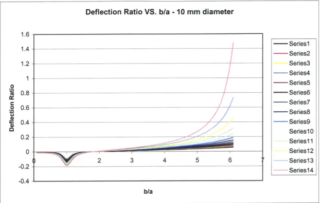
Deflection Ratio VS. b/a - 10 mm diameter 1.6 1.4 1.2 1 0.8 0.6 0.4 0.2 -0.4 - Series1 - Series2 Series3 - Series4 - Series5 - Series6 -- Series7 -- Series8 Series9 Series1I Seriesl3 Seriesl4 0.8 - eri-s 2 3 4 5 6 b/a 10 mm shaft diameter

Deflection Ratio VS. b/a 1.6 1.4 1.2 1 0.8 0.6 0.4 0.2 0 -0.2 -0.4 - Seriesl Series2 Series3 - Series4 - Series5 - Series6 - Series7 - Series8 - Series9 Series12 ---- Series13 --Series14 1. -- eres 0. -- r s 2 3 4 5 6 b/a 8 mm shaft diameter

The above five figures used the following table to construct each series.

Table 9: Values for comparison of the five different diameter shafts, units are in meters. 0 cc .2 Figure 29: 0 .2 0 Figure 30: .. ... " ..... ..

(46)

Series c a 1 0.81 0.076 2 0.79 0.076 3 0.76 0.076 4 0.74 0.076 5 0.71 0.076 6 0.69 0.076 7 0.66 0.076 8 0.64 0.076 9 0.61 0.076 10 0.58 0.076 11 0.56 0.076 12 0.53 0.076 13 0.51 0.076 14 0.48 0.076

As the diameter of the shaft decreases, the air bearing stiffness decreases as well. This is noticeable in the deflection ratio of the above figures. For an 8 mm shaft diameter, the deflection ratio can become as high as 1.4 where for a 25 mm shaft diameter, the ratio is 1. The figures are similar in that they dip down around a b/a ratio of 1 and cross at the x-axis between 2-3. Thus a smaller diameter would work, but the deflection ratio increases at a faster rate than the 32 mm diameter does.

These calculations display an understanding of how a constant shaft diameter works, but the shaft that models the ballscrew-spline is one of two diameters. The next section investigates this.

4.3.5 Variable shaft diameter

The true shaft will have a sleeve on the opposite end of where the ball screw-spline nuts reside. This will make the shaft have a variable cross section. The representation is presented in Figure 31. Y C d D, _D 2 9Ks b

Figure 31: Variable shaft diameter

Splitting the shaft into two sections, one beam with diameter Di and a smaller beam with diameter D2, the overall deflection can be found. It is found by adding the deflection