HAL Id: hal-01399871
https://hal.archives-ouvertes.fr/hal-01399871
Submitted on 21 Nov 2016
HAL is a multi-disciplinary open access
archive for the deposit and dissemination of
sci-entific research documents, whether they are
pub-lished or not. The documents may come from
teaching and research institutions in France or
abroad, or from public or private research centers.
L’archive ouverte pluridisciplinaire HAL, est
destinée au dépôt et à la diffusion de documents
scientifiques de niveau recherche, publiés ou non,
émanant des établissements d’enseignement et de
recherche français ou étrangers, des laboratoires
publics ou privés.
Inverse problem formulation for regularity estimation in
images
Nelly Pustelnik, Patrice Abry, Herwig Wendt, Nicolas Dobigeon
To cite this version:
Nelly Pustelnik, Patrice Abry, Herwig Wendt, Nicolas Dobigeon. Inverse problem formulation for
regularity estimation in images. International Conference on Image Processing (ICIP 2014), Oct
2014, Paris, France. pp. 6081-6085. �hal-01399871�
O
pen
A
rchive
T
OULOUSE
A
rchive
O
uverte (
OATAO
)
OATAO is an open access repository that collects the work of Toulouse researchers and
makes it freely available over the web where possible.
This is an author-deposited version published in :
http://oatao.univ-toulouse.fr/
Eprints ID : 15172
The contribution was presented at ICIP 2014 :
https://icip2014.wp.mines-telecom.fr/
To cite this version :
Pustelnik, Nelly and Abry, Patrice and Wendt, Herwig and
Dobigeon, Nicolas Inverse problem formulation for regularity estimation in
images. (2014) In: International Conference on Image Processing (ICIP 2014),
27 October 2014 - 30 October 2014 (Paris, France).
Any correspondence concerning this service should be sent to the repository
administrator:
[email protected]
INVERSE PROBLEM FORMULATION FOR REGULARITY ESTIMATION IN IMAGES
Nelly Pustelnik
1, Patrice Abry
1, Herwig Wendt
2and Nicolas Dobigeon
21Physics Dept. - ENSL, UMR CNRS 5672, F-69364 Lyon, France, [email protected] 2IRIT, CNRS UMR 5505, INP-ENSEEIHT, F-31062 Toulouse, France, [email protected]
ABSTRACT
The identification of texture changes is a challenging problem that can be addressed by considering local regularity fluctu-ations in an image. This work develops a procedure for lo-cal regularity estimation that combines a convex optimization strategy with wavelet leaders, specific wavelet coefficients re-cently introduced in the context of multifractal analysis. The proposed procedure is formulated as an inverse problem that combines the joint estimation of both local regularity expo-nent and of the optimal weights underlying regularity mea-surement. Numerical experiments using synthetic texture in-dicate that the performance of the proposed approach com-pares favorably against other wavelet based local regularity estimation formulations. The method is also illustrated with an example involving real-world texture.
Index Terms— Local regularity, variational approach, convex optimization, wavelet leaders
1. INTRODUCTION
Wavelet decompositions are now well recognized as sparsify-ing transforms and have been widely used in contexts of im-age compression and restoration [1, 2]. Another very useful property of wavelet transforms found, so far, less widespread use in the field of image processing: their ability to evidence and measure scale invariance (cf., e.g., [3, 4, 5, 6, 7]). No-tably, wavelet transforms have been shown to be relevant tools for the estimation of local regularity [5]. The earliest contri-bution to this subject traces back to [3], where the skeleton (maxima lines across scales) of the continuous wavelet trans-form is shown to enable practitioners to identify irregular (i.e., non-smooth) behavior in signals. By imposing an additional monotonicity constraint on the skeleton, the wavelet
trans-form modulus maxima(WTMM) formalism has been further developed in, e.g., [4] to precisely measure H¨older exponents h. These constitute the canonical theoretical quantities for the measurement of local regularity and for performing multifrac-tal analysis. More recently, it has been shown that accurate es-timates of local regularity can be obtained using wavelet
lead-ers(WL), specific multiresolution quantities that have been demonstrated to precisely reproduce H¨older exponents theo-retically [5, 6]. Wavelet leaders are defined as local suprema This work is supported by the GdR 720 ISIS under the junior research project GALILEO and ANR AMATIS grant #112432, 2010-2014.
of the coefficients of the dyadic wavelet transform and inherit their computational efficiency, see, e.g., [6, 7] and Section 2 below for more precise definition.
Both the WTMM and the WL have been extensively used to perform multifractal analysis of real-world signals and im-ages (see [8, 6, 9, 10] and references therein for examples of successful applications). In contrast to local regularity es-timation, multifractal analysis does not aim at the time- or space-resolved estimation ofh but rather provides a global and geometric description of the fluctuations ofh in an image in terms of the so-called multifractal spectrum. However, for certain applications, the central information of interest is pre-cisely the evolution along time or space of the H¨older expo-nent. In this case, multifractal analysis is not directly relevant. Instead, direct estimation of the local regularity evolution, sometimes referred to as multifractional analysis, needs to be performed. Yet, the estimation ofh at a precise time/space location suffers from poor performance that impairs its actual practical use. Consequently, the estimation of the time/space evolution of local regularity remains barely used in applica-tions (see, a contrario, [11, 12]). In particular, local estima-tion of regularity suffers from a large variance and common post-processing techniques for variance reduction, such as lo-cal smoothing, induce significant bias in the estimation ofh and inaccuracies in the localization of changes in regularity.
In a previous contribution [13], we have proposed an orig-inal two-step procedure that addresses the bias-variance trade-off difficulty in the specific context of images with piece-wise constant regularity: (i) Unbiased estimation of the H¨older ex-ponent for every position in the image using a patch-based wavelet leaders approach, (ii) Extraction of areas with uni-form H¨older exponent from these local estimates using a vari-ational procedure relying on total-variation (TV) [14]. In the present contribution, we elaborate on this approach and propose a one-step procedure that directly yields piece-wise constant local regularity estimates. The originality of the ap-proach resides in combining estimation ofh and the TV de-noising in a single-step. Through this formulation, an effi-cient local regularity estimation procedure is designed, yield-ing significantly increased estimation quality for images with piece-wise constant texture.
The remainder of this work is organized as follows. Sec-tion 2 recalls the noSec-tion of H¨older exponent, defines wavelet leaders and the state-of-the-art H¨older exponent estimation
procedure. Section 3 formalizes the estimation of local reg-ularity explicitly as an inverse problem and details the pro-posed variational procedure. Section 4 reports experimen-tal results illustrating the performance of the proposed piece-wise constant regularity estimation/segmentation procedure.
2. H ¨OLDER EXPONENT AND WAVELET LEADERS Loosely speaking, the H¨older exponent h(x) is a positive quantity that measures the regularity of a function at location x ∈ R2by comparing the evolution along scale of multireso-lution quantities (cf. (2)) aroundx against a local power law behavior (see [5] for a precise definition). Qualitatively, a small value of the H¨older exponent indicates a locally highly irregular behavior, close to discontinuous, of the function, while a large value indicates local smoothness. A simple, ef-ficient and theoretically well grounded solution to practically computeh(x) relies on the use of wavelet leaders [6], which we define in what follows. Note that it has recently been proven [5] that wavelet leaders enable to measure the H¨older exponent for much more general classes of bi-dimensional functions than wavelet coefficients, and with a significantly improved accuracy [5, 6, 7, 13].
Letf denote the bi-dimensional function taking bounded values (i.e, the image) to be analyzed. Letφ and ψ denote respectively the scaling function and mother wavelet defining a 1D multiresolution analysis. The corresponding 2D ten-sor product wavelets are defined, for everyx = (x1, x2) ∈ R2, as: ψ(0)(x) = φ(x
1)φ(x2), ψ(1)(x) = ψ(x1)φ(x2), ψ(2)(x) = φ(x
1)ψ(x2), and ψ(3)(x) = ψ(x1)ψ(x2). The collection ψ(m)j,k (x) = 2−jψ(m)(2−jx − k) of dilated (to scales2j) and translated (to space positions2jk) templates of ψ(m) form a basis ofL2(R2) for well chosen functions ψ. The (L1-normalized) discrete wavelet transform (DWT) coefficient at scalej, location k and subband m ∈ {1, 2, 3} is defined asd(m)(j, k) = hf, 2−jψ(m)
j,k i.
The wavelet leader coefficientL(j, k) is defined, for each scalej and location k, as the local supremum of all wavelet coefficients taken within a spatial neighborhood across all finer scalesj′≤ j L(j, k) = sup m={1,2,3} λj′ ,k′⊂Λj,k |d(m)(j′, k′)|, (1) whereλj,k= [k2j, (k+1)2j) and Λj,k =Sp∈{−1,0,1}2λj,k+p [5, 6]. For everyx ∼ 2jk, the wavelet leaders reproduce the H¨older exponenth(x) as follows:
L(j, k) ≃ C(x)2jh(x) (2) when2j → 0 and where C(x) denotes a constant. This rela-tion can be rewritten as:
ln L(j, k) ≃ jh(x) + ln C(x), (3)
which naturally leads to the use of linear regressions across scales at each locationk ∼ 2−jx for the estimation of h(x), i.e.,
bh(x) =X j
w(j, k) ln L(j, k). (4) Taking the expectations of (3) and (4) above yields
Ebh(x) = h(x)X j
jw(j, k) + ln C(x)X j
w(j, k), (5) thus showing that the constraints
X j
w(j, k) ≡ 0 and X j
jw(j, k) ≡ 1, (6) ensure an unbiased estimation ofh. Due to their local nature involving only a small number of coefficients, the estimates (4) have large variance. A straightforward attempt to reduce the variance consists in local spatial averaging (smoothing) ofh(x). However, local smoothing induces bias and prevents from accurately locating changes ofh in the image. To over-come this difficulty, a total variation (TV) optimization pro-cedure, naturally favoring sharp edges, has been proposed in [13]. It requires the use of estimates ofh(x), which are ob-tained using (4) with fixed pre-defined weightsw(j, k). Al-though this approach yields relevant results, it does not enable to distinguish areas with H¨older exponents that are too close in value because the variance of (4) is too large.
In order to reduce the variance of (4), one can attempt to optimize the weightsw(j, k) which reflect the confidence granted to the quantitiesln L(j, k). The variance of ln L(j, k) depends on the value of the H¨older exponenth(x) at loca-tionk ∼ 2−jx and the optimal choice of the weights w(j, k) thus varies from one location to the other. Therefore, we pro-pose in this article to formulate the estimation ofh(x) as an inverse problem involving jointly the H¨older exponentsh(x) and the weightsw(j, k) (constrained only by (6)) as parame-ters to be estimated. The inverse problem formulation and the proposed proximal based minimization procedure for finding its solution are detailed in the following section.
3. INVERSE PROBLEM BASED LOCAL REGULARITY ESTIMATION
“Degradation” model From now on, we make use of a discrete time formalism. Letf = (f [n])1≤n≤N denote the vector representation of the image to be analyzed, of size N = N1× N2. The orthonormal wavelet transform is labeled F ∈ RN×N and the wavelet coefficients of f are denoted d = (d[n])1≤n≤N = F f . At each scale j ∈ {1, . . . , J}, Lj : RN → R2
−2jN
denotes the non-linear transform that associates the wavelet coefficients to the wavelet lead-ers Lj = (Lj[k])1≤k≤2−2jN (as defined in (1)) such that Lj= Lj(F f ). A matrix formulation of (4) leads to:
j2
X
j=j1
with1 ≤ j1< j2≤ J and where ε models the uncertainties in the estimation, mostly due to the finite range of available scales. For each j ∈ {j1, . . . , j2}, Wj ∈ RN×N denotes a diagonal matrix whose diagonal values are the regression weights, i.e, Wj = diag(wj) with wj = (wj[n])1≤n≤N ∈ RN, andD
j ∈ RN×2
−2jN
denotes a matrix that duplicates the signal such that, for every(u, v) ∈ R2−2jN
× RN, if we denote u ∈ R2−jN
1×2−jN2 (resp. v ∈ RN1×N2) the
ma-trix representation ofu (resp. v), v = Dju means that, for every(n1, n2) ∈ {1, . . . , N1} × {1, . . . , N2}, v[n1, n2] = u!⌈2−jn
1⌉, ⌈2−jn2⌉".
The model in (7) underlies an inverse problem in which h = h([n])1≤n≤N need to be recovered from the logarithm of the wavelet leaders coefficients (ln Lj)j1≤j≤j2. This
in-verse problem resembles a denoising problem, yet including the additional challenge that a part of the observations (the regression weights matrices (Wj)j1≤j≤j2) is unknown and
must satisfy constraints (6).
Variational approach We propose to estimate the local regularityh and the regression weight matrices (Wj)j1≤j≤j2
by solving the following minimization problem:
!"h, #W$∈ Argmin h,W % % % j2 X j=j1 WjDjln Lj− h % % %2 2+ λTV(h) + η1 N X n=1 dC1(w[n]) + η2 N X n=1 dC2(w[n]) (8)
whereW = (Wj1, . . . , Wj2) and thus w[n] = (wj1[n], . . . ,
wj2[n]) belongs to R
j2−j1+1. The first term denotes a data
fidelity term. Distances to the convex setsC1andC2, denoted dC1anddC2, are introduced to provide some flexibility in the
hyperplane constraintsC1andC2:
C1= {(ωj1, . . . , ωj2) ∈ R × . . . × R | j2 X j=j1 ωj = 0}, C2= {(ωj1, . . . , ωj2) ∈ R × . . . × R | j2 X j=j1 jωj = 1}. For everyw ∈ R(j2−j1+1),d C1(w) = %w − PC1(w)%, with PC1(w) = arg minv∈C1%w − v%
2, denotes the projection onto the convex set C1 (resp. dC2 and PC2). The second
term TV(h) acts as a penalization that forces a solution with a minimal total variation [14] that is, for everyh ∈ RN,
TV(h) = %T h%2,1= N X n=1 # |(Hh)[n]|2+ |(V h)[n]|2 (9) where T = [H⊤V⊤]⊤ withH ∈ RN×N andV ∈ RN×N are matrix representations of, respectively, the horizontal and vertical first-order discrete differences. The parametersλ, η1, andη2will impact directly the solution. One could note that the choice of parametersλ = 1/η1= 1/η2 = 0 leads to the standard estimation procedure, formulated in (4) and (6).
Proximal algorithm The minimization problem (8) is con-vex but smooth. In the recent literature dedicated to non-smooth convex optimization, several efficient algorithms have been proposed. For instance, when a Lipschitz data fidelity term is involved, such as a quadratic data fidelity term, as well as several regularization terms, such as TV regularization or distance to convex sets, one suited algorithm is referred to as CV (for Condat-V˜u) [15, 16]. The corresponding iterations tailored to solve the problem in (8) are given in Algo. 1, that ensures convergence of the sequence(h[ℓ], W[ℓ])
ℓ∈Nto a so-lution of (8).
Algorithm 1 Algorithm for solving (8)
Initialization Set σ >0 and τ ∈(0, 1 kPj2j=j1Djln Ljk2+1+2σ ) . Set h[0]∈ RN , w[0]= (w[0]j1, . . . , w [0] j2) ∈ R N(j2−j1+1), u[0]= (u[0]j1, . . . , u [0] j2) ∈ R N(j2−j1+1), and y[0]∈ R2N. For ℓ= 0, 1, . . . For j= j1, . . . , j2 * Uj[ℓ]= diag(u[ℓ]j ) Wj[ℓ]= diag(w [ℓ] j )
⋆ Gradient descents steps ⋆ h[ℓ+1]= h[ℓ]− 2τ!h[ℓ]−+j2 j=j1W [ℓ] j Djln Lj $ − τ T⊤y[ℓ] For j= j1, . . . , j2 * , Wj [ℓ] = Wj[ℓ]− 2τ ! +j2 j=j1W [ℓ] j Djln Lj− h[ℓ]$(Djln Lj)⊤− τ Uj[ℓ]
⋆ Proximity operator step based on dC1⋆
For every j, we denotew-[ℓ]j the diagonal values of ,Wj[ℓ] w[ℓ+1]=!proxτ η1dC1( -w [ℓ] j1[n], . . . , -w [ℓ] j2[n]) $ 1≤n≤N
⋆ Proximity operator step for TV on h ⋆ p[ℓ]= y[ℓ]+ σT (2h[ℓ+1]− h[ℓ])
y[ℓ+1]= p[ℓ]− σprox
σ−1λk·k2,1(σ −1p[ℓ])
⋆ Proximity operator step for dC2⋆
q[ℓ]= u[ℓ]+ σ(2w[ℓ+1]− w[ℓ]) u[ℓ+1]= q[ℓ]− σprox η2dC2 σ ! σ−1(q[ℓ] j1[n], . . . , q [ℓ] j2[n]) $ 1≤n≤N
Algo. 1 requires the computation of the proximity oper-ators associated to the mixed ℓ2,1-pseudo norm and to the distance to convex sets. Let us recall that the proximity op-erator associated to a convex, lower semi-continuous convex functionϕ from H (where H denotes a real Hilbert space) to ]−∞, +∞], denoted proxϕ, is defined as, for everyu ∈ H, proxϕ(u) = arg minv∈H12%u − v%2+ ϕ(v). When ϕ de-notes the indicator function of a non-empty closed convex set C ⊂ H, that is ιC(x) = 0 if x ∈ C and +∞ otherwise, the proximity operator reduces to the projection, denotedPC, onto the convex set.
The proximity operator steps involved in Algo. 1 have a closed-form expression. Indeed, it is shown in [17], that for everyu = (u[n])1≤n≤N withu[n] ∈ R2,
proxλ σ$·$2,1u = $ max(0, 1 − λ σ%u[n]%)u[n] % 1≤n≤N (10)
−20 0 20 0.3 0.4 0.5
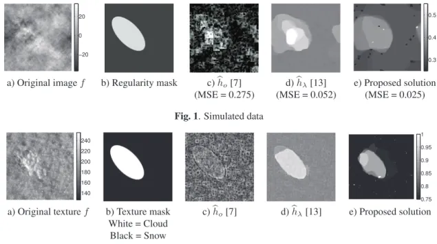
a) Original imagef b) Regularity mask c) bho[7] d) bhλ[13] e) Proposed solution (MSE = 0.275) (MSE = 0.052) (MSE = 0.025) Fig. 1. Simulated data
140 160 180 200 220 240 0.75 0.8 0.85 0.9 0.95 1
a) Original texturef b) Texture mask c) bho[7] d) bhλ[13] e) Proposed solution White = Cloud
Black = Snow
Fig. 2. Real data Moreover, according to [18, Proposition 2.8], ifC denotes a
non-empty closed convex subset of R(j2−j1+1)and ifη > 0,
for everyu ∈ R(j2−j1+1), proxηdCu = & u +η(Pc(u)−u) dC(u) if dC(u) > η, PC(u) if dC(u) ≤ η. (11) For our purpose,C models the hyperplane constraints C1and C2and one could note thatPC1andPC2 have a closed form
expression given in [19].
4. EXPERIMENTAL VALIDATION
We first evaluate the performance of the proposed estimat-ing strategy on synthetic data, consistestimat-ing of 2D multifrac-tional Brownian fields [20, 21], whose definition has been slightly modified here to ensure an homogeneous variance across the image (cf. [13] for details). The synthetic pro-cess has piece-wise constant regularity according to the mask shown in Fig. 1-b), with h = 0.5 in the central area and h = 0.3 for the background. A sample field is displayed in Fig. 1-a).
Analysis is conducted using a standard2D DWT with or-thonomal tensor product Daubechies mother wavelets with2 vanishing moments. Regularity is estimated using the scal-ing range(j1, j2) = (2, 4). We compare the performance of the solution proposed against two other approaches. First, a standard estimation procedure with a priori fixed weightswj chosen to achieve ordinary linear regression, labelled bho, (re-sults are plotted in Fig. 1-c)). Second, we evaluate the perfor-mance of the technique proposed in [13] consisting in com-puting the proximity operator of the total variation of bho, i.e, proxλTV(bho). The solution of this latter method is labelled
bhλ (cf., Fig. 1-d)) and the parameterλ is empirically tuned to minimize the normalized mean square error (MSE) in this second approach. The solution proposed in Section 3, whose result is depicted in Fig. 1-e), achieves a smaller MSE and better evidence of the central area.
A second experiment deals with real data, obtained by mixing textures. The image is generated by inclusion of a distinct ellipse-shaped zone of cloud texture in a snow tex-ture background (cf. Fig. 2-a)). First, it is worth noting that the unbiased local regularity estimation in Fig. 2-c) allows the edges of the added areas to be identified. However, without these synthetic edges, the local regularity change is difficult to identify. Similar observations are made for the solution ob-tained with [13], shown in Fig. 2-d) and the proposed solution. However, the proposed solution provides a better discrimina-tion with sharper edges.
5. CONCLUSION
An efficient local regularity estimation strategy adapted to a multifractional framework has been devised. It enriches the classical estimation procedure by including the estimation of the weights that enter the linear regressions. These extra de-grees of freedom yield local regularity estimates with signif-icantly reduced variance. The proposed estimation procedure is formulated as an inverse problem and is solved using prox-imal minimization. Numerical experiments indicate that the proposed procedure significantly outperforms the standard es-timation procedure and to further improve eses-timation perfor-mance compared to an earlier TV based procedure. Moreover, local regularity is also shown to be efficient to discriminate between visually similar textures such as cloud and snow.
6. REFERENCES
[1] S. Mallat, A wavelet tour of signal processing, Aca-demic Press, San Diego, USA, 1997.
[2] M. N. Do and M. Vetterli, “The contourlet transform: an efficient directional multiresolution image represen-tation,” IEEE Trans. Image Process., vol. 14, no. 12, pp. 2091–2106, Dec. 2005.
[3] S. Mallat and S. Zhong, “Characterization of signals from multiscale edges,” IEEE Trans. Pattern Anal. Match. Int., vol. 14, no. 7, pp. 710–732, 1992.
[4] J.F. Muzy, E. Bacry, and A. Arn´eodo, “Wavelets and multifractal formalism for singular signals: Application to turbulence data,” Phys. Rev. Lett., vol. 67, no. 25, pp. 3515–3518, 1991.
[5] S. Jaffard, “Wavelet techniques in multifractal analy-sis,” in Fractal Geometry and Applications: A Jubilee
of Benoˆıt Mandelbrot, Proceedings of Symposia in Pure Mathematics, M. Lapidus and M. van Frankenhuijsen, Eds. 2004, vol. 72, pp. 91–152, AMS.
[6] H. Wendt, P. Abry, and S. Jaffard, “Bootstrap for empir-ical multifractal analysis,” IEEE Signal Process. Mag., vol. 24, no. 4, pp. 38–48, Jul. 2007.
[7] H. Wendt, S.G. Roux, P. Abry, and S. Jaffard, “Wavelet leaders and bootstrap for multifractal analysis of im-ages,” Signal Proces., vol. 89, pp. 1100–1114, 2009. [8] A. Arneodo, N. Decoster, and S.G. Roux,
“Inter-mittency, log-normal statistics, and multifractal cas-cade process in high-resolution satellite images of cloud structure,” Phys. Rev. Lett., vol. 83, no. 6, pp. 1255– 1258, 1999.
[9] A. Echelard and J. L´evy V´ehel, “Self-regulating processes-based modeling for arrhythmia characteriza-tion,” in Imaging and Signal Processing in Health Care
and Technology, Baltimore, United States, May 2012. [10] P. Abry, S. Jaffard, and H. Wendt, “When Van Gogh
meets Mandelbrot: Multifractal classification of paint-ing’s texture,” Signal Process., vol. 93, no. 3, pp. 554– 572, 2013.
[11] B. Pesquet-Popescu and J. L´evy Vehel, “Stochastic frac-tal models for image processing,” IEEE Signal Process.
Mag., vol. 19, no. 5, pp. 48–62, Sep. 2002.
[12] O. Pont, A. Turiel, and H. Yahia, “An optimized algo-rithm for the evaluation of local singularity exponents in digital signals,” in Combinatorial Image Analysis, J.K. Aggarwal et al., Ed., vol. 6636 of Lecture Notes in
Computer Science, pp. 346–357. Springer Berlin Hei-delberg, 2011.
[13] N. Pustelnik, H. Wendt, and P. Abry, “Local regular-ity for texture segmentation: Combining wavelet leaders and proximal minimization,” in Proc. Int. Conf. Acoust.,
Speech Signal Process., Vancouver, Canada, May 2013, pp. 5348–5352.
[14] L. Rudin, S. Osher, and E. Fatemi, “Nonlinear total vari-ation based noise removal algorithms,” Physica D, vol. 60, no. 1-4, pp. 259–268, Nov. 1992.
[15] L. Condat, “A primal-dual splitting method for convex optimization involving Lipschitzian, proximable and linear composite terms,” J. Optim. Theory Appl., vol. 158, no. 2, pp. 460–479, 2013.
[16] B. C. V˜u, “A splitting algorithm for dual monotone in-clusions involving cocoercive operators,” Adv. Comput.
Math., vol. 38, pp. 667–681, 2011.
[17] G. Peyr´e and J. Fadili, “Group sparsity with overlapping partition functions,” in Proc. Eur. Sig. Proc. Conference, Barcelona, Spain, Aug. 29 – Sept. 2, 2011, pp. 303–307. [18] P. L. Combettes and J.-C. Pesquet, “A proximal decom-position method for solving convex variational inverse problems,” Inverse Problems, vol. 24, no. 6, pp. 065014, Dec. 2008.
[19] S. Theodoridis, K. Slavakis, and I. Yamada, “Adaptive learning in a world of projections,” IEEE Signal
Pro-cess. Mag., vol. 28, no. 1, pp. 97–123, Jan. 2011. [20] A. Benassi, S. Jaffard, and D. Roux, “Gaussian
pro-cesses and pseudo-differential elliptic operators,” Rev.
mat. Iberoamericana, vol. 8, no. 1, pp. 19–89, 1997. [21] A. Ayache, S. Cohen, and J. L´evy Vehel, “The
covari-ance structure of multifractional Brownian motion, with application to long range dependence,” in Proc. Int.
Conf. Acoust., Speech Signal Process., Dallas, Texas, USA, Mar. 14-19, 2000, pp. 3810–3813.