Computation of safety control for hybrid system with applications to intersection collision avoidance system

Computation of Safety Control for Hybrid System with

Applications to Intersection Collision Avoidance System

by

Geng Huang

Submitted to the Department of Mechanical Engineering

in partial fulfillment of the requirements for the degree of

ARCHIVES

Master of Science in Mechanical Engineering

_{MASSACHUSETS INSTITUTE}

OF TECHNOLOGY

at the

OCT 0

12015

MASSACHUSETTS INSTITUTE OF TECHNOLOGY

September 2015

LIBRARIES

@

Massachusetts Institute of Technology 2015. All rights reserved.

Signature redacted

Author...

Department of Mechanical Engineering

August 7, 2015

Certified

by...Signature

redacted

Domitilla Del Vecchio

Associate Professor

Thesis Supervisor

Accepted by

...

...

David Hardt

Chairman, Department Committee on Graduate Theses

Computation of Safety Control for Hybrid System with

Applications to Intersection Collision Avoidance System

by

Geng Huang

Submitted to the Department of Mechanical Engineering on May 8, 2015, in partial fulfillment of the

requirements for the degree of

Master of Science in Mechanical Engineering

Abstract

In this thesis, I consider the problem of designing a collision avoidance system for the scenario in which two cars approach an intersection from perpendicular directions. One of the cars is a human driven vehicle, and the other one is a semi-autonomous vehicle, equipped with a driver-assist system. The driver-assist system should warn the driver of the semi-autonomous vehicle to brake or accelerate if potential dangers of collision are detected. Then, if the system detects that the driver disobeys the warning, the system can override the behavior of the driver to guarantee safety if necessary. A hybrid automaton model with hidden modes is used to solve the problem. A disturbance estimator is used to estimate the driver's reaction to the warning. Then, with the help of a mode estimator, the hybrid system with hidden modes is translated to a hybrid system with perfect state information. Finally, we generalize the solution for the application example to the solution of safety control problem for general hybrid system with hidden modes when the hybrid system satisfies some proposed constraints and assumptions.

Thesis Supervisor: Domitilla Del Vecchio Title: Associate Professor

Acknowledgments

Through the support and help of many people, this thesis was made possible.

I would like to thank my parents and family for their love and support. They gave me

the chance to get a good education, develop my ability, and realize my potential. All the support they have provided me over the years was the greatest gift anyone has ever given me.

I would like to thank my thesis advisor, Professor Domitilla Del Vecchio, for her guidance,

understanding, and support.

I would like to thank Daniel Hoehener, who gave me so many valuable advices, and

helped me substantially in the development of theory in this thesis.

I would like to thank all of my friends. It was these friends who made my success more

enjoyable, and cheered me up when I failed.

I would thank NSF-CPS Award 1239182 for the support of my research. This funding

allowed me to pursue and investigate research topics showed in this thesis.

Finally, I would like to express my gratitude to the MIT School of Engineering, and the Department of Mechanical Engineering, who gave the wonderful resources for studying, and working.

Contents

1 Introduction

2 Motivation Example 3 System Model

3.1 The structure of hybrid automaton .... ... 3.2 The execution of hybrid automaton ...

4 Problem Formulation

5 Solution to Problem 1 6 A Disturbance Estimator

6.1 Problem Statement and Assumptions . . . .

6.2 A State and Disturbance Estimator . . . . 7 Mode Estimation

8 Transformations from H to H 9 Simulation Example

9.1 Model of Finite State Machine H . . . .

9.2 Construction of Estimation Finite State Machine . . . . 9.3 Sim ulation Results . . . .

10 Conclusion and Future Work

11 17 21 22 23 27 29 41 41 43 45 47 51 51 53 56 67

List of Figures

2-1 Problem scenario for intersection collision avoidance . . . . 2-2 System H . . . .

8-1 Calculate the value function using results from disturbance and 8-2 System f . . . . 9-1 9-2 9-3 9-4 9-5 9-6 9-7 mode estimator Problem scenario . . . . System H . . . . System H... ... R anged2(hol) . . . . R anged2(ho2) . . . .

Worst case disturbance profile of d2 for getting trapped in hol Worst case disturbance profile of d2 for getting trapped in ho2

9-8 Initially, both of the two cars are human driven and the mode of the system

is h. . . . .

9-9 When the red trajectory goes through the point (L1, U2), the value of the

value function is 0, and the control signal o," 2 should be applied. . . . .

9-10 The mode of the system has been switched to w2. The system will stay in W2

for time TRT . . . . . . . . . .. . . . . . - . - . . . . .. . . . . ...

9-11 Disobeying the accelerating warning is detected. . . . . 9-12 After disobeying accelerating warning is detected, the mode of the system

will be switched to hd2. The blue dashed trajectory is generated using the

maximum control for a2. . . . .

. . . . 18 . . . . 19 49 50 . . . . 52 . . . . 52 . ... 54 . . . . 54 . . . . 55 . . . . 56 . . . . 56 58 59 60 61 62

Chapter 1

Introduction

Improving driving safety is one of the main takes in developing road vehicles. Lots of atten-tions have been given to vehicle safety since the 1960's 125, 31]. The introductions of passive

safety features such as seat belts, air bags and advanced lighting systems have substantially reduced the rate of crashes [17, 221. However, despite the significant improvements, each year in United States, collisions of motor vehicles still result in 40,000 deaths, more than three million injuries, and over $130 billion in financial losses

[4,

17]. Since the development

of passive safety system could not provide further significant improvements in vehicle safety, the development of active safety protection system became the new trend of vehicle safety system development [29J. Different from passive safety system that reduces injuries of pas-sengers in crash; active safety protection systems prevent potential crashes by warning the driver [261. One of active safety protection systems is automotive collision avoidance system. Automotive collision avoidance system actively warns drivers of a potential collision event, allows the driver adequate time to take appropriate actions to avoid the collision event [11]. Numerical analysis of collision data strongly suggests that automotive collision avoidance system can tremendously reduce collisions [11]. Crash data collected by the U.S. National Highway Traffic Safety Administration (NHTSA) show that automotive collision avoidance system can theoretically prevent 37% to 74% of all police reported rear-end crashes [22, 35]. It can be seen that the introduction of collision warning systems resulted in significant re-duction of crash fatalities, injuries, and property damage.

demonstrate the importance and benefits of the research on intersection collision avoidance system. However, due to the complicatedness of designing intersection collision avoidance systems and the limitations of the radar technology, intersection collision avoidance systems received less attention than the forward collision avoidance systems

[471.

Thanks to vehicle-to-vehicle communication technologies, the development of intersection collision avoidance systems became practical [21, 261. Previous research results show that it is possible to detect threats of collision by vehicles cooperatively sharing critical information, such as location, velocity and acceleration [30, 45, 28]. By sharing the information, each vehicle is able to predict the potential collision [30, 45]. However, the effectiveness of this technology depends on the percentage of vehicles on the road using it and the number of vehicles equipped with navigation and communication systems

[311.

The Cooperative Intersection Collision Avoidance System for Violations (CICAS-V) project conducted by Mercedes-Benz Research and Development North America, Inc. developed a prototype system to prevent crashes by predicting stop-sign and signal controlled intersection violations and warning the violating driver [251.

In this thesis, we consider the design of intersection collision avoidance system involving a normal human driven vehicle and a vehicle equipped with the intersection collision avoidance system. When the potential of collision is detected, the system warns the driver (to accelerate or brake) based on the positions and velocities of the two cars. After receiving the warning, the driver has adequate time to react. Then, the system will estimate the driver's reaction to the warning, and the system can override the behavior of the driver if the driver disobeys the warning and a collision is about to happen. The scenario after the driver receives the issued waring can be divided into three sub-cases depending on the reaction of the driver regarding to the system warning of a potential collision. First, the driver obeys the warning and cross the intersection safely. Second, the driver disobeys the warning but could safely pass the intersection. Third, the driver ignores the warning in an unsafe condition and a crash is

possible. Then the driver assist system will give the vehicle a control input to avoid collision

by overriding the input from the driver. In some cases, the driver obeys the warning at the

beginning, and later he/she disobeys the issued warning. This case is regarded as that the driver disobeys the warning from the assist system. In order to guarantee the effectiveness of the system, the design of the intersection collision avoidance system needs to be provable safe.

Also, in the collision warning system design, human factors play an important role

[34].

The purpose of the warning is to alert the driver when there is a potential of collision and the driver is unaware of it

[47].

A collision waning system should detect both the

potential of collision and the driver's reactions regarding the collision warning and collision possibility

[461.

If the driver has already taken an appropriate action, the intervention from

the collision avoidance system should be discarded to reduce the annoying factor 1221. Also, a good warning system should minimize the additional attention load for the driver

[46].

A system that gives excessive warning or overriding may desensitize and distract the driver and decrease the driving satisfaction [22]. Undesired warnings and overriding may also make the driver turn off the system completely [461. Thus, it is important to design a collision system which is least conservative. A least conservative system requires that the control actions will only be taken when safety cannot be guaranteed otherwise.

Hybrid automaton is used to model the intersection collision avoidance system involving a human driven vehicle and a semi-autonomous vehicle with the collision avoidance system (driver assistance system) installed. Hybrid automaton can model continuous vehicle dynam-ics as well as discrete human decisions and overriding decisions from the driver assistance system [33, 361. These features make it an ideal framework for the modeling, since driver usually switch between different driving actions [38]. Also, there are a lot of development of modeling and control techniques for hybrid systems that can be utilized.

Research has been done in the safety control problem for hybrid systems with perfect state information, with imperfect continuous state information, and with unknown modes when all transitions are driven by unknown disturbance events [39, 24].

There are numerous research results on safety control problem for hybrid systems in which modes and state information are well known [24, 20, 12, 2, 3, 37, 32, 141. The hybrid

have been working on approximate solutions to calculate the maximal controlled invariant set [18, 1]. Also, the termination of the computation of the maximal controlled invariant set has been investigated and works have been done to find special cases of the systems, for which termination can be proved

[321.

The hybrid system control problem with imperfect state information has also been ad-dressed [8, 9, 7, 15, 16, 131. In those works, the mode of the system is assumed to be known but there are uncertainties in the continuous state. The controller is designed based on a state estimator for finite state systems [8, 9, 15, 14, 131. Linear complexity state estimation and control algorithms are proposed for hybrid systems with order preserving dynamics [8, 9, 15, 131.

The intersection collision avoidance system design problem is formulated as a hybrid controller design problem for hybrid automaton in which modes are hidden since driver's decisions are unobservable and uncontrollable.

The hybrid system control problem for guaranteeing safety with unknown modes has been investigated in [40, 39, 41, 42, 43, 44]. There are literatures studying Hidden Mode Hybrid Systems (HMHSs), in which the mode is unknown and mode transitions are driven only

by disturbance events [40, 391. The lack of knowledge of mode and disturbance transition event gives a control problem with imperfect mode information. The control problem with imperfect mode information is translated to problem with perfect state information using derived deterministic or probabilistic information state [40, 39, 41]. The derived non-deterministic information state tracks all possible states compatible given the history of the system [40, 39, 41]. With the update law for the derived information state, the control problem can be reconstructed using the new derive states, and the problem becomes hybrid control design problem with perfect state information [40, 39, 41J.

Control design problem for driver assistance system which gives driver warnings before overriding can be modeled as hybrid systems with hidden modes. Hybrid systems with

hidden modes are special cases of hybrid automata. In hybrid systems with hidden modes, some modes are unknown and some mode transitions are driven by disturbance events. In this document, we consider mode transitions can be either driven by disturbance events or control events. Also, we consider the case such that the allowed ranges for continuous input signals are mode and time dependent. Warning and active safety systems for vehicle collision avoidance need to guarantee safety in the presence of human drivers, whose driving decisions and behaviors are unknown and are modeled as disturbance transition events and continuous disturbance signals. Also, in order to co-operate the design of warning the driver and overriding when needed, control events are modeled to trigger transitions between some modes. Continuous control signals are also involved in the system dynamics to fulfill the functionality of overriding. Thus, we study hybrid systems in which mode transitions can be driven by both unknown disturbance events and designed control events. Also, continuous disturbance and control signals are both involved in the system dynamics.

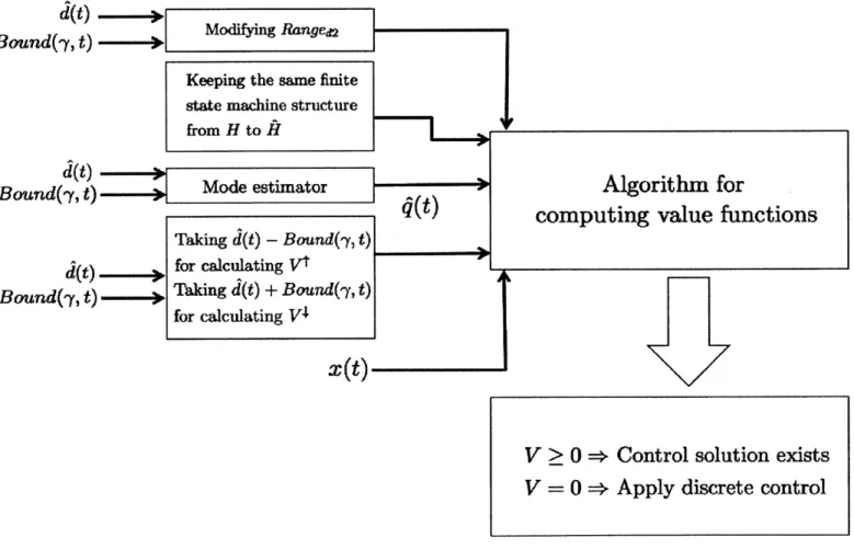
To solve the problem, first, we propose a hybrid control solution assuming all states and signals are well measured. Then, we consider the case in which disturbance transition events, mode of the system, and continuous disturbance signals are not known. We assume that the continuous state is well known. A disturbance estimator is used to estimate the continuous disturbance signals and further its results are used to estimate the mode of the system given the relationship between continuous disturbance signals, the disturbance transition events and the mode of the system. With the estimated mode, a new hybrid system with perfect knowledge about mode and transitions are constructed. Then, we modify the inputs to the hybrid control calculation algorithm based on the estimated values. Finally, a hybrid feedback control map is designed to prevent the flow of the system from entering the collision set for the current time and all future time.

Continuous state information, i.e., positions and velocities of the two vehicles, is assumed to be available. The continuous state information of the normal human driven vehicle could be provided by cameras and vision systems located at the intersection [21, 34, 28]. Using vehicle-to-infrastructure communication technologies, short range communications devices (dedicated short range communication 5.9 GHz in the United States) can distribute the state information to the driver assistance system installed on the semi-autonomous vehicle [47, 29,

Chapter

2

Motivation Example

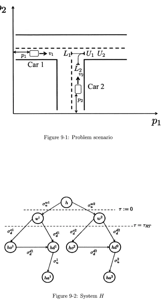
We consider the scenario in which two cars approach an intersection from perpendicular directions. One of the cars is a human driven vehicle, and the other one is a semi-autonomous vehicle, equipped with a driver-assist system, referred to as controller in the following. The

controller takes measurements of positions and speeds of the two cars as inputs. If, based on the inputs, the controller detects the potential of collision, it can issue braking or accelerating warnings to the driver of the semi-autonomous vehicle. After issuing the warnings, the controller uses its inputs (positions and speeds) to estimate whether the driver obeys the issued warning. If disobeying is detected, the controller can override the driver whenever this should become necessary.

In order to design the controller on the semi-autonomous vehicle, we model the whole system as a hybrid automaton, which will be introduced in the next section. The continuous dynamics of the system are the following.

The human driven vehicle is referred as Car 1 and the semi-autonomous vehicle is referred as Car 2. For i = 1, 2, we use pi, vi, and ai to denote the position, speed, and acceleration of car i along its path. For t > 0, we have

A (0) = Vi(0) (2.1)

P,0 -* vi L, U1 U2

Car l

L2

Car 2

P1

Figure 2-1: Problem scenario for intersection collision avoidance

We assume that the acceleration a1(t) at time t E R+ of the human driven vehicle

is determined by a disturbance signal di(t). Similarly, the acceleration a2(t) of the

semi-autonomous vehicle at time t

e

R+ is determined by a disturbance signal d2(t) if the system

is not in override mode and by a control signal u(t) otherwise. Both disturbance and control

signals are assumed to be bounded, i.e., di(t), d2(t) E [-d, d] and u(t) E [-ii, i] for all t E R+. Defining the intersection as Int = (L1, U1) x (L2, U2

),

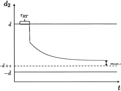
the objective of the controller is to guarantee that (p1(t), P2(t)) Int for all t > 0.

The warning and override mechanism is modeled as a finite state machine shown in Fig. 2-2. Initially, both cars are human-driven, and we denote that mode as h. If the potential danger of collision is detected, braking or accelerating warning will be issued to the driver of the semi-autonomous vehicle. In the following, we describe warning/overriding mechanism assuming an braking warning is issued, left branch of the tree in Fig. 2-2. The case of an accelerating waring is analogous, except that in the notation a superscript 1 is replaced with a superscript 2, right branch of the tree in Fig. 2-2. Issuing a braking warning results in a mode transition from h to mode w'. We define the time instance at which a warning is

issued as t := 0. After receiving the warning, the driver of the semi-autonomous vehicle needs time rRT to react, so the system will stay in mode w' for time [0, rRT). When t =TRT,

the reaction time has passed and the driver should react to the issued warning. Obedience to the warning is represented by the discrete disturbance signal uo and will trigger the mode transition from w' to ho'. Similarly, if the driver disobeys the braking warning, the disturbance signal ar will trigger the mode transition from w' to hd'. hd1 means that the driver has disobeyed the warning, and if necessary, the control system can override the driver of the semi-autonomous vehicle to guarantee safety. If disobeying braking warning has been detected, when necessary, a will be issued and the mode of the system will be switched ha1.

iurl 2-2 Ss

Chapter 3

System Model

We start by introducing the notation of hybrid automaton.

Definition 1. A hybrid automaton is a tuple H = (Q, X, U, D, EU, Ed, R,

f)

in which

Q

is

the finite set of system modes with q E

Q;

X is the space of continuous states with x E X; U is the set of continuous control inputs with u

E

U; D is the set of continuous disturbance

inputs with d E D; EU is the finite set of discrete control inputs with o- E Eu; Ed is the

finite set of discrete disturbance events with 0-d E Ed; R : Q x Eu x Ed -+

Q

is the mode update map;

f

: X x

Q

x U x D --+ TX is the vector field with I f(x, q, u, d) and TX is

a tangent space of X.

In the example discussed in Section 2, we have Q {h, w1, w2, hol, hd1, ho2, hd2, ha', ha2}. Pi

X C IV and x = .Eo1f2 d2}. D c R2 and U c R1. E =

P2

V2

{wlf, og2, oj, o-}. f is mode transition map in Fig. 2-2 and f is the longitudinal continuous

dynamics of the two cars given in Eq. 2.1 and 2.2.

In this thesis, we define the (Q, E = Ed x Eu) as a directed acyclic graph (DAG). In

the following, we will first introduce the structure of the hybrid automaton and then the execution of it.

For vertices u and v, we have u < v if there exists a directed path from u to v.

For a signal a and a time interval T, we define a(T) to be the sequence of signal a in the time interval T. Starting from a state qo, we define

#q(t,

qO, Ou([0, t)), OdO([0, t))) := q(t) for t > 0 as the discrete flow of the system. Based on the partial order property of DAG, we

have qO < q(t).

Definition 2. For a set of mode

Q

with partial order property, we define min(Q) = q if

Vq'

C

Q,

q' > q. We define max(Q) = q if Vq' c Q, q > q'.

Here, we introduce some notations that are going to be used in the subsequent sections.

Definition 3. For a node q E

Q,

we define

i DisturbancefReach(q) = {q' I ]Ud s.t. R(q, 0, o-d) q'}. ii Control Reach(q) =

{q'

I Bo-, s.t. R(q, o-, 0) q'}. iii DSR(q) = {q' ]

It

and Od([0,t)) s.t.

0q(t,q,O,

o-d([0, t)))= q'} U {q}.

For example, we have DisturbanceReach(w2_{) ={ho}2_{, hd}2_{} and DSR(w}2_{) {W}2_,

ho2, hd2}. ControlReach(w2) =0 and ControlReach(hd2) = {ha21.

Definition 4. We say that a node q E

Q

is a head if ]q' s.t. q E ControlfReach(q'). In the example, tv1 and w2 are both head.

For a node q which is a head, we call DSR(q) as a Connect(q).

Definition 5. For a node q which is a head, we define

i Branch(q) =

{q'

E Connect(q)IControl Reach(q') = 0}.

We denote a mode q as a qlast if ControlReach(q) = 0 and DisturbanceReach(q) = 0.

In the example, hal and ha2 are both qiast.

Assumption 1. For each node q E

Q,

at least one of DisturbanceReach(q) and ControlReach(q) is empty.

This implies that for all nodes q E Q, the links directed from q can be either a discrete

disturbance transition or a discrete control transition, but not both.

Assumption 2. For all q₁, q2 C

Q,

Control Reach(q1)

n

Disturbance Reach(q2) = 0.

Assumption 2 implies that a node cannot be reached by both a discrete disturbance signal and a discrete control signal.

3.2

The execution of hybrid automaton

Here, we consider the execution of the hybrid automaton.

We define R(q, 0,0) = q for all q E

Q.

The sequence {Ti}ieN+ with 0 < Ti < Ti+1 represents the sequence of times at which node transitions occur with (o(Ti), Od(Ti)) 74

(0,

0)

and (ou(t), (d(t)) = (0, 0) for all t {Ti}iEN+. We define the discrete trajectory q(t) of system

H as follows.

Given q(0) = qo, we define q(t) = qO for 0 < t < T1. If Ti

#

ri+1, then we define q(t) = R(q(Ti),U.(Ti),o-d(Ti)) for t E (Ti,7ri+11. If for some i C N+, Ti = Ti+1

Ti+k = > 0 with k E N+ and finite, then k

+

1 mode transitions occur at time T. For

J E {1, 2, 3, ... , k + 1}, we define (o-(T)j, -d(T)j) as the discrete signals triggering the j-th mode transition occurring at time T. Also, we define q(T)j as the mode after the j-th

mode transition happening at time 7. Then we have q(T)1 = R(q(T), O-u(T)1, d(T)1), and

q(T)m+ = R(q(T)m, u ()m, Od(T)m) for m E {1, 2, 3,... , k}. We define q(t) = q(T)k+1 for

For the continuous trajectory x(t) E X of system H, given x(0) = xo, (t) = f(x(t), q(t), u(t), d(t)) with u(t) E U and d(t) E D. Starting from xO and qO, we define

of q. If at time instance ti, the mode of system H is transited to q, q(tj) = q, then for T E [ti, ti + DT(q)), we have (o(T), -d(T)) = (0, 0), and (oa(ti + DT(q)), o-d(tl +

DT(q)))

#

(0, 0).

(2) if DTF(q) = 0, then mode q does not have dwell time.

In the example, DTF(wl) =1 and DTF(w2) = 1 with DT(wl) = DT(w2) = TRT. This means that after receiving the issued warning, the driver has time rRT to react. Within the reaction time, the driver's behavior is not used as driver's reaction to the warning. All of the other modes do not have dwell time.

Assumption 3. For any mode q E

Q,

if DTF(q) = 1, then there exists q'

C

Q

such that q C CantrolfReach(q').

Assumption 4. For a mode q E

Q,

if DTF(q) = 1 and DisturbanceReach(q)

$

0, then there exists a q' E DisturbanceReach(q) such that DisturbanceReach(q) C DSR(q').

Definition 6. For a mode q and q'

E

DisturbanceReach(q) with DTF(q) = 0, the boundary

between Ranged2(q) and Ranged2(q'), which is denoted as BRd2(q, q') is defined BRd2(q, q')

ORanged2(q)

n

Ranged2(q).

For a mode q

C

Q

and a mode q'

C

DisturbanceReach(q),

" if DTF(q) = 0, then the discrete disturbance signal od which transits the mode from q to q' is applied if and only if the continuous disturbance signal d2 cross the boundary

of Ranged2(q) and Ranged2(q'), BRd2(q, q'), and go from Ranged2(q) to Ranged2(q')I

" if DTF(q) = 1, then the discrete disturbance signal Ud which transits the mode from

q to q' is applied if and only if DT(q) is reached and d2 go from a value in Ranged2(q)

Assumption 5. For a mode q

C

Q such that there exists a q' with DTF(q') = 0 and q E DisturbanceReach(q'),

" Ranged2(q) V Ranged2(q');

" at least one of sup Ranged2(q) > sup Ranged2(q') and inf Ranged2(q) < if Ranged2(q')

is true;

" furthermore, if sup Ran ged2(q) > sup Ran ged2(q'), then for qf C DisturbanceReach(q), we have sup Ranged2(qn) > sup Ranged2(q); if inf Ranged2(q) < inf Ranged2(q'), then

for qf C DisturbanceReach(q), we have inf Ranged2(q) < inf Ranged2(q).

Assumption 6. For all qi,q3 E DisturbanceReach(q) with DTF(q) = 0, Ranged2(qi) n Ranged2(qj) C Ranged2(q).

Definition 7. For each mode q E Q, we define Ranged(q) C D as the set of allowed

continuous disturbance signals associated with mode q, and we define Rangeu(q) C U as the set of allowed continuous control signals associated with mode q.

For example, Ranged(ho2) = [-, d] x [j- e, d] and Rangeu(ha2) [-].

Assumption 7. We consider the continuous dynamic of system H to be composed by two parallel systems S1 and S2. For i = 1, 2, we define system Si as the following:

xij(t) = Ai(q(t))xi(t) + Bi(q(t))di(t) + Ei(q(t))uilt) (3.1)

yi(t) = Cixi(t) (3.2)

where di, ui E R. x, EI R', A1(q) is a m x m matrix, B1(q) and E1(q) are m x 1 matrices, x2 E

Rn , A2(q) is a n x n matrix, B2(q) and E2(q) are n x 1 matrices. di(t) E Rangedi(q(t), t) C

R where Rangedi(q(t), t) is the allowed range for di(t) in mode q(t) at time t. ui(t) C Rangeu2(q(t), t) C R, and Rangeu(q(t),t) is the allowed range for ui (t) in mode q(t) at time

t. C1 and C2 are 1 x m and 1 x n matrices respectively.

In the example, we have A1(q) = A2(q) =

[

,

B1(q) -

H

and EI(q(t)) = for

We define C = C Any composed signal a of S1 and S2 are composed in a

0 C2

way such that a (a,, a2). For example, x = (x1, x2) is the composed continuous state

of the system and y = (yi, Y2) is the composed output signal. We have y = Cx. Also,

d(t) = (d1(t), d2(t)) E Ranged(q(t), t) = Rangedl(q(t), t) x Ranged2(q(t), t) and u(t) =

(ui(t), u2(t)) E Ranges(q(t), t) = Range,,(q(t), t) x Rangen2(q(t), t).

Assumption 8. For any mode q E

Q

with the following properties

i 3q1 E

Q

with q E DisturbanceReach(q1) or Eq2 E

Q

with q2 E DisturbanceReach(q), ii DTF(q) 0,

we require

|d

2

|

< 3(q) where 3(q) E R+ defines the allowed range for d2 in mode q.

Assumption 9. For any Connect, we have Vq1, q2 G Connect, i 13(qi) = /3(q2

)-ii A2(qi) = A2(q2), B2(q1) = B2(q2), and E2(q1) = E2(q2).

Assumption 8 and 9 specify some requirements on S2, and for S1, there are no such requirements.

Assumption 10. For Si, Vt > 0, if VT E [0, t), Uia(T) Uib(T), dia(T) > dib(T), and Xia(0) > xib(0), then we have yia(t) > yib(t).

Chapter 4

Problem Formulation

In this section, we formulate the problem we want to solve.

We start by defining a set Bad C R2 such that Bad = (L1, U1) x (L2, U2) with U1 > L, > 0 and U2 > L2 > 0.

Notice that the set Bad is an open rectangular set in R2.

Problem 1. With (C1x1(0), C2x2(0)) V Bad, for any t > 0, given q(t), x(t) and d(t) with

d(t)

c

Ranged(q(t)), for all T > t, design a least conservative control map 7F : X x

Q

x D -+ U x E, i.e., (u([t,T)), o-u([t, T))) = 7r(x(t), q(t), d(t)), such that (CiX1(T), C2x2 (T)) V Bad,

Vd([t, T)) and U-([t, T)).

Here, the least conservative control map means that the control actions will only be taken if the continuous flow cannot be guaranteed to be kept outside Bad otherwise.

Chapter 5

Solution to Problem 1

We define

B-

= (-oo, UI) x (L2, 00),

so we have Bad = Bt

n

Bt. We define the safe set for a set K given an initial disturbance

signal do and a mode qo as

W(K, do, qo) = {xoJVt > 0, ]u([0, t)), and o-,([0, t)) s.t. Vud([0, t)) and d([0, t)) with

d(0) = do, Cox (s, xo, qo, u([0, t)), d([0, t)), u([0, t)), d([0, t))) K Vs C [0, t)}.

Lemma 1. W(Bad, do,q) =W(B,do,q)U W(B,do, q).

Proof. The statement W(Bad, do, q) ; W(Bt, do, q) U W(B, do, q) follows immediately from Bad c Bt and Bad C B1. Hence it suffices to show W(Bad, do, q) C; W(B, do, q) U W(B , do, q).

We pick any xo = (xoi,X02) E W(Bad, do, q).

Then, for all t > 0, there exists u([0, t)) and ou([0, t)) s.t. for all 0d([0, t)) and d([0, t)) with d(0) = do, C#x(s, xo, qo, u([O, t)), d([0, t)), o-([0, t)), od([0, t))) Z Bad = Bt n Bt for all s E [0, t).

Let's assume C1xo1 < U1 and C2x0 2< U2. Otherwise, the proof will be trivial because Bt = (L 1, oo) x (- oc, U2)

We denote t1 as the first time instance such that Cixi(ti) > L1. Then, because both C₁x₁(t) and C2x2(t) are continuous increasing functions with respect to time, we have either

C2x2(ti) < L2 or C2x2(t1) > U2.Similarly, we denote t2 as the time instance with C1x1(t2) U1. Then, we have either C2x2(t2) < L2 or C2x2(t2) > U2.

Since both Cixi(t) and C2x2(t) are continuous increasing functions with respect to time,

if C2X2(t1) < L2, then for all ti < T < t2, we have C2x2(r) < L2. If C2x2(t1) > U2, then for

all t1 < T < t2, we have C2x2(T) > U2.

In the case of C2x2(t1) < L2, for all 0 < t < ti and t > t2, Cx(t) V B . When t1 < t < t2,

Cx(t) V B . Thus, in this case, xo C W(B , do, q). Similarly, in the case of C2x2(t1) U2,

c0

E W(Bt, do, q).

As a result, xo E W(Bt, do, q) U W(B4, do, q). ]

For a set K and a point x, we define distK(X) - infkEK ix - ko. For a set K, we define the oriented distance function from x to K as bK(X) distK(x) -

distKc(x)-Given a finite state machine H, a point xo, a mode q and do E Ranged2(q), we define the value functions [10, 23]

VH (xo, q, do) = max min min bBad(Cx(t,xo,qou([O,t)),d([O,t)),

u([qoo)),o) ([,om)) d([m,oo)),mt([q,0()) t[E)[O,o() 07u([O, t)), 9d([0, O)))

Vt (xo, q, do) = max min min bBC2t xo, qo, u([0, t)), d([0, t)), H ~u([,oo)),as ([o,oo)) d([o,oo)),0s ([0,0o)) t E [0,00) BT( (t

V (xo, q, do) = max min min bi (Cx(t, xo, qo, u([0, t)), d([0, t)),

u([0,oo)),o. ([0,oo)) d([0,oo)),Oad ([0,oo)) tE [0,0o)

au([0, W), o-d([0, t))))

where o and gd trigger the mode transitions in H, u and d are selected in the allowed ranges

for specific modes in H, and d2(0) = do. Then, we have W(Bad,do,q) = W(BT, do, q) = W(B1, do, q) = {xo|VH(xo, q, do) > 01 {x0 V$(xo, q, do) > 01

{xoV (xo, q, do) > 0}.

Corollary 1. For a finite state machine H, a point xo, a mode q and do G Ranged2(q) compatible with q, {xo|VH(xo, q, do) > 0} {xoI max(V4 (xo, q, do), V' (xo, q, do)) > 0}.

Proof.

W(Bad, do, q) = {xoVH (xo, q, do) > 0}

= W(Bt, do, q) U W(B , do, q)

{xo0IV(xo, q, do) > 0} U {xoV (xo, q, do) 01 {xo Imax(V (xo, q, do), V (xo, q, do)) 01.

In the following, we will only show the case for Bt, and the case for B can be done similarly.

For each Connect in the finite state machine, we consider a mode (denoted as q,) such

that for all q e Connect with DTF(q) = 0, qh Disturbance Reach(q), and DTF(qh) = 0.

If

|DisturbanceReach(qh)I

> 1, then for q* E DisturbancefReach(qh) with inf Ranged2(q*) >

inf

Ranged2(qh), we remove all q' with q' > q* from the finite state machine. We denote the

to ChildCOannect and we use qp to denote the mode such that gend E DisturbanceReach(qp) and DTF(qp) = 0. We define qn to be the head of the ChildConnect, and we define

d* = inf Ranged2(qn).

Now, we consider two cases: DTF(q) = 0 and DTF(q) = 1.

(1) DTF(q) =0.

We define ttran do-infRanged2(qp) if do > inf Ran ged2(qp), and we define ttay

d₀-inf Ranged2(qend)

Then, we define u4

ran ([0, ttran)) (Utranl ([0, ttran)), Utran2 ([0, ttran))) and dXran([0, ttran))

(d'irani([0, ttran)), dtan₂([0, ttran))) such that for T E [0, ttran)

(a) u'rani (T) = inf Range,, (q)

(b) Ulran2(T) = sup Rangeu2(q)

(c) dani(T ) sup Rangedl(q)

(d) dXran2(r) = do - ,B.

We define

Xon Ox (ttrani xo, q, tran( [0, ttran) ), d,-an ( [0, ttran)), 1, 0 7 ran [0,1 ttran))

with o~tran([0, ttran)) being compatible with dpan([0, ttran)).

For t > 0, we define utay([0, t)) (U' ay([0, t)),tay₂([0,t))) and ditay([0,t)) (dtayi([0, t)),diay2([0, t))) such that for T

C

[0, t)

(a) usitayi(r) = inf Rangeui(q)

(b) U'tay2() = sup Rangeu2(q)

(d) dita,2(r) = max(do - /3r, inf Ranged2(qend))

-For t > 0, we define

darstet) = de (Cst(y q, 3,(0 (1, 1)) disay([0, 7 )), 0, 7 ,dtsay([0, t))))

with ,stay([0, t)) being compatible with dstay([0, t)).

Also, for t > 0, we define u'([0, t)) - (u' ([0, t)), u'([0, t))) and d,([0, t)) = (dj,([0, t)), d'([O, t))) such that for T E [0, t)

(a) ut (T) inf Range,1 (q) (b) Un (T) sup Rangeu2(q)

(c) d'(-r) sup Rangedl(q)

(d) d2 (T) max(do - Or, inf Ranged2(q)).

For t > 0, we define

dB-tc(t) = dBT (C#x(txo, q, ul([0,t)), dic([0, t)), 0, a Q-(0, t))).

with oc([0, t)) being compatible with dc([0, t)).

It should be noted that if the current mode q is gend and ControlReach(q) # 0, then being trapped in the current Connect is not possible . In this case, qp does not exist, and we define mint dBTc(t) = 00.

(2) DTF(q) =1.

Definition 8. NoTranDT(q) = { q'Iq' E DisturbancefReach(q) and Control Reach(q') =

0}.

Now, we use qt to denote max(NoTranDT(q)).

We denote the time the mode has stayed in q as RT, and we denote RT = DT(q) - RT, as the remaining time the mode will stay in q. We define ttran =

(b) uran2(T) = sup Rangeu2 (q)

(c) d4 _{anI (T) sup Ranged1 (q)}

(d) dtran₂(T) inf Ranged2(q) if T r [0, RT] and dctan2(T) = infRanged2(qt)-/3(T-RT)

if T G (RT, RT + ttran). We define

XOn =#x(RT + ttran, tran ( [0, RT + ttran)),

d4ran( [0, RT + ttran)), 0, OJtran( [0, RT + ttran)))

with odtran( [0, RT + ttran)) being compatible with

d4ran

([0, RT + ttran)).

For t > 0, we define ultay([Ot)) = (U'tayi([i, t)), Utay₂ [0, t))) and ditay([O, t)) (datayi([, t)), ditay2([, t))) such that for T E [0, t) with t > RT

(a) ustayl (T) inf Rangeu, (q) (b) U'1tay2(T) sup Rangeu2(q)

(c) dtayl(T) = sup Rangedl(q)

(d) dtay2(T) inf Ranged2(q) if T E [0, RT1. If T > RT, then

i if gend DisturbanceReach(q), then ditay 2(T) max(inf Ranged2(qt)

- 3(T - RT),

inf Ranged2(qend));

ii if gend E DisturbanceReach(q), then ditay₂ (T) inf Ranged2 (qend).

For t > 0, we define

with atostay([O, t)) being compatible with dtay ([0, t)).

Also, for t > 0, we define u,([O, t)) = (Uz4([0, t)), u([0, t))) and d(0, t)) =

(d([O, t)), d 2([0, t))) such that for T c [0, t) with t > RT

(a) ut (T) = inf Ran geu (q)

(b) 'a (T) = sup Rangeu2(q) (c) d'1(T) sup Rangedl(q)

(d) dT₂(T) inf Ranged2(q) if T

C

[0, RT] and d 9( ) =

max(inf Ranged2(qt) - O(T - RT), inf Ranged2(qp)) if T> RT1.

For t > 0, we define

dB~ctc dBT CX(t, X0, q, u ([0, t)), d c([0, t)), 0, a1Q0, t))).

with o([0, t)) being compatible with dl([, t)).

It should be noted that if qt or qp does not exist, then being trapped in the current Connect is not possible. In this case, we define mint dBtc(t) = oo.

For any xo, do and H, we define VH(xo, 0, do) = -oo.

Proposition 1. V$(xo, q, do) = min(max(mint dBstay(t), MaXq, EControl Reach(qend)

VT (xon, qn, d*)), mint d c(t)), where end c DSR(q) and DisturbanceReach(qend) 0.

Given the current mode of the system, we can determine the Connect the mode is in. Then, there are three options we have.

(1) The mode of the system transits within NotTran(q) and the mode of the system is

trapped in the current Connect without the ability to transit to other Connects. If stay-ing within NotTran(q) gives a negative value function, which means that mint dc(t) < 0,

then the whole value function will have a negative value and no control map can guar-antee safety.

(2) The mode of the system transits to Branch(q). Now, the controller can decide whether to stay in the mode of Branch(q), or transit the next Connect, based on which way

the end, if the system reaches the Connect from which no more Connect transitions are possible, and staying in that Connect is not safe, then the value function has a negative value, and no control map can guarantee safety.

In order to prove Proposition 1, we will first introduce the following propositions. Based on the following propositions, Proposition 1 is a direct result.

Proposition 2. For all t > 0, if for all 0 < s < t, we have ul(s) = (u'(s),u'(s)) and u2(s) = (u2(s), u2(s)) such that ul(s) > u2(s) and ul(s) < u2(s), and d1(s) = (d'(s), d'(s))

and d2(s) = (d2(s),d2(s)) such that dl(s) < d2(s) and d'(s) > d2(s), then starting from

XO = (XOi, X02), using the same continuous dynamics, we have dB-((y'(t), y'(t)))

d ((y2(t), y2(t))), where (yl(t), y'(t)) is the point reached using ul and d', and (y2(t), y2(t))

is the point reached using us and d2

Proof. By the order preserving property, it is know that yj(t) y (t) and y' (t) K y (t).

By the definition of the oriented distance function, dBt ((yi (t), y2(t))) either equals to L, -yi(t) or y2(t) - U2. Since L, - yl(t) < L, - y2(t) and y1(t) - U2 < y2(t) - U2, we have

dBT ((Y1 M, Y2 (0) < dBr (y2 (t, y2 (t))

-What we have shown implies that staying in the same Connect (which means that the same continuous dynamics are used), decreasing ul, increasing u2 will increase the value

function and increasing di, decreasing d2 will decrease the value function.

For any t > 0, if we are given u-([0, t)) and u([0, t)), then Proposition 3 follows directly

from Proposition 2.

For t > 0, if we are given od([0, t)) and uo([0, t)), then for each time instance t > 0, we have ui(t)

c

[u'(t), u (t)], u2(t) E [u'(t), uu(t)], d1(t)

c

[d'(t), du(t)] and d2(t) E [d'(t), du(t)].

If we are given the upper and lower bounds for u1, U2, d, and d2, for t > 0, we define

'u

t_{([0,t)) = (ul(i0,t)),u'([0,t))) such that for all} T E [0, t), we have ul(r) = u'(7) and

u (r) uu (r). Also, we define d([0, t)) = (d ([O, t)), d([0, t))) such that for all r E [0, t),

we have d'(T) = du(r) and d4(r) = d'(T).

Proposition 3.

max min min but (C#,(t,

xo,

go, uT([0, t)),

i([0,

t)), O-u([0, t)), O-d([0, t))))

u([O,oo)) d([O,oo)) tE[O,oo)

=min bBT (C#x (tx o g,a QT(0, t)), jd([O, t)) , O-u ([0, t)), i -([O, t)))). tE [O,oo)

Notice that if we are given U([0, t)) and

uo([O,

t)), then for each time instance, we need to

pick the optimal continuous control and disturbance signals to optimize the oriented distance. If U-d([, t)) and o-,([, t)) are not given and we need to pick optimal od([0, t)) and ou([O, t)) to optimize the value function, then we optimize the value function by changing the bounds for the continuous signals u([O, t)) and d([O, t)) using Jd([O, t)) and o- ([O, t)).

From Proposition 2, another result we have is the following proposition.

Proposition 4. Vlj;(xo, q, do) = VT (xo, q, do). Hcut

Proof. From Proposition 2, it is known that the disturbance signals minimize the value

function by picking the minimal continuous disturbance signal at each time instance. Thus, the node removed from H will never be reached and considered in the calculation of the value function because going through those removed nodes will increase the minimal continuous disturbance signal we can pick. As a result, the value function calculated considering H will be the same as the value function calculated considering H t.

Given the current mode of the system, the mode of the system will either get stuck in the current Connect or reach a mode, from which either the mode of the system can go to another Connect, or no more transitions are possible. The discrete disturbance signal will select among getting stuck and go to "the last" mode of the current Connect in order to minimize the value function. If the mode of the system reaches the last mode of the current

Connect, then the discrete control signal will select whether to stay or go to the following Connect in order to maximize the value function. Thus, we have Proposition 1.

Proof. If VH(xo, q, d₀) > 0, then we know that there exist control signals, such that no

matter what disturbance signals are applied, on trajectories of (yi, Y2), the point which is most closed to the set Bad has a positive distance from the set Bad. Among the trajectories, let us pick the trajectory whose most closed point to Bad has the smallest distance. This trajectory corresponds to the best case control and worst case disturbance. We denote that

point as CXd = (C1Xd1, C2Xd2). There exists a J > 0 and a neighborhood Ne(CXd)6 around

CXd such that for any point y* c Ne(Cd), I Cxd - y* I 6 and bBad(y*) > 0. Let's denote

infy*ENe(Czd)6 bBad(y*) Crid. For a trajectory of (Y1, Y2) (denoted as TJ), we define the

distance from the trajectory TJ to the set Bad as infpETj bBad(P). Because both yi and Y2 are continuous with respect to time and increasing, then there exists a neighborhood around

Cx0, such that trajectories of (y1, y2) starting from any point in the neighborhood have a

minimum distance greater or equal than Crid. Since both yi and Y2 are continuous with respect to time, then there exists an s s.t.,

VH (#x (s, X, U([0 , s)) , d([0 , s)), 0, -([0, s))),

,

(q, 0, a(Q0, s))), do (s)) > 0

for all d([0, s)) and ad([0, s))).

It should be noted that if the controller is able to apply discrete control signals to switch

Connect, then the mode of the system has arrived to a qend which is a Branch mode as

defined in Definition 5. When the mode of the system has arrived qend, and no discrete

control signals are applied, then in the future, applying the discrete control signals is still possible.

Proposition 6. For all s > 0, there exists O([0, s))) and corresponding dt Q0, s)) such that

do(s))-Proof. This is trivial from the definition of the value function since by applying 0o', we try

to maximize the value function. El

In the calculation of the value function, it is assumed that q and d2 are measured. In

that case, given a finite state machine H, we can calculate the value function to find the control map. However, if d2 and q are not directly measured, then we need to modify the

hybrid system so that we can still use the solution to Problem 1 to find the control map. In the next section, we will introduce a disturbance estimator to estimate d2. Then,

based on the estimation of d2, we will construct a hybrid system based on H with modified

Chapter 6

A Disturbance Estimator

In this section, we will introduce a disturbance estimator presented in

[5].

6.1

Problem Statement and Assumptions

We consider systems described by

=Ax + Bd +Wu (6.1)

y = Cx (6.2)

where x(t)

E

R' is the system state and y(t) E RP is the measured output at time t E R. The continuous control signal u(t) E R' models the control inputs to the system, and the continuous disturbance signal d(t) E R'" models all uncertain in the system and it is regarded as an unknown state-independent time-varying input. A, B, C and W are known constant real matrices.

In order to estimate x(t) and d(t), we need the following two assumptions.

Assumption 11. rank(CB) = rank(B).

Assumption 12. For every complex number A with nonnegative real part,

A -AXI B

rank( ) = n + rank(B).

We C 0

(2) Find F, L, and C such that

P(A + LC)+(A + LC)T P < 0

f3Tfj - GC.

To do that, we need to follow the following steps. (a) Choose L22 such that A22 + L22C22 is Hurwitz.

(b) Choose P22 > 0, then P = I* 0 (c) Define

Q22

= -[ P22(A22 + L2 2C2 2) + (A2 2 + L2 2C2 2)T P221 > 0 Qn - Al + AT + (A₁₂+ AT P₂₂)Q₂1(A T + P_{2 2}A_{2 1})

Choose n > Ama(Q"). Then we have L

(d) Make C = _BTC1

₀₁

(3) The transformations

P = (T T P)-I T-1 L = TLS-1 G = GS- 1.

transform F,

Z,

and C to P, L, and G.

(6.3a) (6.3b) (6.3c) [KC-1 0 0 L22 (6.4a) (6.4b) (6.4c)

6.2

A State and Disturbance Estimator

We construct the state and disturbance estimator as follows.

x = A + Bd +Wu + L(C: - y) (6.5a)

d =--G(C - y) (6.5b)

where -y is a positive scalar, the initial estimate -(to) = o is arbitrary, and :(t) and d(t) are the estimates of x(t) and d(t) respectively. We need j|d(t)I| < 01 and

|ld(t)II

< 2.

We define a = 2 > 0 and a = (

)

. Based on the analysis in

[5],

by making

22 o

-y > max {8, $- } where p1 and [2 are two non-negative real numbers which can be chosen

arbitrarily. We define

11 + (to)-Q ItoI

Bound(-y, t) = a{2Ba (A + LeC)[ ) +11e(to)11e- +-' B()]+ [()i + 11e(to)I e--)1}.

(6.6)

Chapter

7

Mode Estimation

In this section, we consider the construction of a mode estimator based on the result from the disturbance estimator.

It should be noted that mode estimation is needed

* when the mode of the system is in a Connect, whose head qh does not have dwell time, contains more than one mode;

" or when the mode of the system is in a Connect, whose head qh has dwell time, contains

more than two modes.

Let's consider the mode of the system is in a Connect which satisfies the two conditions for requiring mode estimation, and we define the time instance at which the mode of the system enters the Connect as T= 0. We record the time instance for entering the Connect

as t*. The disturbance estimator is started when T = 0. It should be noted that the time

instance in the Connect, r, corresponds to a time instance t for running the whole hybrid system with the relationship t = t*

+

T.

Given the Connect q(t) is currently in, we use the following algorithm to calculate q(t). Given a Connect, we use NoDT Mode(Connect) =

{

q

E

Connect|DTF(q) = 0}.

When the dwell time of the head has passed, we will begin to do the mode estimation.

If head does not have dwell time, then we start mode estimation as soon as the mode of the

system enters the Connect.

6: end while 7: end procedure

Corollary 2. For t > 0, we have q(t) E 4(t).

Corollary 2 shows that the mode estimator is a correct estimator since the true of the system is always contained in the estimated modes.

Chapter 8

Transformations from H to H

In this section, we consider how to construct the hybrid system H based on the structure of

H.

From system H to H, the structure of the finite state machine remains the same. The ranges for ul, U2 and d, in corresponding modes are the same. We need to modify the evoking conditions for discrete disturbance transitions and Ranged2 for each mode.

For each mode q E H, we label the mode of H at the corresponding position as q. For the evoking conditions for discrete disturbance transitions, since the disturbance transitions events and the continuous disturbance signals cannot be directly measured, we use the mode estimation method introduced in the previous section to determine whether there will be a mode transition in system H.

For each Connect, we define the time instance at which the mode of the system enters the Connect as T = 0, and the disturbance estimation is started at T = 0. For two modes qi and q2 in the Connect with q2 E DisturbanceReach(q1) and DTF(q1) = 0 and DTF(q2) = 0,

" if sup Ranged2(q2) > sup Ranged2(ql), then the event inf dRange(r) > sup Ranged2(q1)

triggers the mode transition from qi to 2;

" if sup Ranged2(q2) < sup Ranged2(qi), then the event sup dRange(r) < inf Ranged2(ql) triggers the mode transition from 41 to 62.

For a mode q E

Q

with dwell time, the corresponding mode E

Q

0 has the same dwell