HAL Id: inria-00402079
https://hal.inria.fr/inria-00402079
Submitted on 20 May 2011
HAL is a multi-disciplinary open access
archive for the deposit and dissemination of
sci-entific research documents, whether they are
pub-lished or not. The documents may come from
teaching and research institutions in France or
abroad, or from public or private research centers.
L’archive ouverte pluridisciplinaire HAL, est
destinée au dépôt et à la diffusion de documents
scientifiques de niveau recherche, publiés ou non,
émanant des établissements d’enseignement et de
recherche français ou étrangers, des laboratoires
publics ou privés.
Fast Hydraulic Erosion Simulation and Visualization on
GPU
Xing Mei, Philippe Decaudin, Bao-Gang Hu
To cite this version:
Xing Mei, Philippe Decaudin, Bao-Gang Hu. Fast Hydraulic Erosion Simulation and Visualization
on GPU. PG ’07 - 15th Pacific Conference on Computer Graphics and Applications, Oct 2007, Maui,
United States. pp.47-56, �10.1109/PG.2007.15�. �inria-00402079�
Fast Hydraulic Erosion Simulation and Visualization on GPU
Xing Mei
CASIA-LIAMA/NLPR, Beijing, China xmei@(NOSPAM)nlpr.ia.ac.cn
Philippe Decaudin
INRIA-Evasion, Grenoble, France & CASIA-LIAMA, Beijing, China
philippe.decaudin@(NOSPAM)imag.fr
Bao-Gang Hu
CASIA-LIAMA/NLPR, Beijing, China hubg@(NOSPAM)nlpr.ia.ac.cn
Figure 1. Illustration of our erosion simulation on a ”PG”-shaped mountain. (a) The initial terrain. (b) Terrain is being eroded by rainfall. The dissolved soil (denoted by green color) is transported by the water flow (blue). (c) The eroded terrain and the deposited sediment (red) after the rainfall and during the evaporation.
Abstract
Natural mountains and valleys are gradually eroded by rainfall and river flows. Physically-based modeling of this complex phenomenon is a major concern in producing re-alistic synthesized terrains. However, despite some recent improvements, existing algorithms are still computationally expensive, leading to a time-consuming process fairly im-practical for terrain designers and 3D artists.
In this paper, we present a new method to model the hy-draulic erosion phenomenon which runs at interactive rates on today’s computers. The method is based on the velocity field of the running water, which is created with an efficient shallow-water fluid model. The velocity field is used to cal-culate the erosion and deposition process, and the sediment transportation process. The method has been carefully de-signed to be implemented totally on GPU, and thus takes full advantage of the parallelism of current graphics hard-ware. Results from experiments demonstrate that the pro-posed method is effective and efficient. It can create realis-tic erosion effects by rainfall and river flows, and produce fast simulation results for terrains with large sizes.
1. Introduction
Natural terrains exhibit a lot of complex shapes such as valleys, ridges, sand ripples and crests. These geomor-phological structures are mostly determined by the erosion phenomenon: soil is dissolved and transported by the wa-ter flow, sand is carried away by the wind, and stones are decomposed into small blocks by the temperature. Erosion simulation has always been an important research topic in landscape design [5, 8], since it greatly enhances the realism of the synthesized terrains.
We focus on hydraulic erosion, which is the predominant cause of erosion for most outdoor landscapes [9]. It de-scribes how the soil on the terrain is dissolved, transported and deposited by the running water, as described in Sec-tion 3. Many algorithms have been proposed to simulate this complex process [2, 19, 20, 24]. Although they produce realistic eroded terrains, they are usually computationally expensive, leading to computation time varying from min-utes to hours on common computers. This is inconvenient for terrain designers, who wish to view the dynamic sim-ulation process and edit the parameters interactively. Fur-thermore, we notice that the topographical changes of the terrain also affect the distribution of the water flows.
In-cluding the erosion effect in fluid simulation will greatly enhance the realism of the running water on terrains, such as rivers, brooks and even lavas. Less work has been done on this problem [6, 7, 17].
In this paper, we propose a fast method for hydraulic ero-sion simulation, in order to get immediate simulation results for interactive applications. Our first concern is to design an algorithm that can take full advantage of the high par-allel computing power offered by today’s graphics process-ing units (GPU). We represent terrain and water surfaces as height fields on 2D regular grids. Then we adapt a shallow water model from [22] to update the water surface and the fluid velocity field. To the best of our knowledge, this model has not been used for erosion simulation before. Based on the velocity field, we calculate the amount of the eroded soil and the deposited sediment in each cell of the grids. Follow-ing the erosion-deposition process, the suspended sediment is transported by the velocity field. With careful design, the values in the grid cells can be updated in parallel at each step, which fits well into the general computing framework of the current graphics hardware [11, 23]. Therefore the simulation model is implemented on GPU as a multi-pass algorithm, and the simulated results can be directly used for visualization. Relying on GPU’s parallelism and flexible programmability, our method provides significantly faster results than previous methods while preserving the realism. This allows us to create fluvial eroded terrain and view all the important features for erosion in real-time, such as water movement and catchment, evaporation, soil dissolving and sedimentation.
The rest of the paper is organized as follows. In Sec-tion 2, we review the related work. In SecSec-tion 3, we present our model in detail. The multi-pass implementation on GPU is given in Section 4. In Section 5, we present the experi-ment results and performances for several examples. Fi-nally we conclude our work in Section 6.
2. Related Work
Many erosion algorithms have been proposed in the field of soil science and computer graphics [9, 28]. Some early methods adapt the fractal rules with ad hoc changes to produce eroded terrains from scratch. Kelly et al. [14] created a drainage network of the rivers with geological data, and then generated fractal terrain around this network. Prusinkiewicz and Hammel [24] integrated rivers into their mountain models by applying midpoint displacement with predefined water basins.
More algorithms try to simulate the erosion process with physically based models and modify the relief of the already-existing terrains. Musgrave et al. [19] described a general framework for physically based erosion model-ing. Some material is dissolved and transported by the
ter flow, and finally deposited at another location. The wa-ter movement is dewa-termined by local gradient of the wa-terrain in a simple diffusion algorithm. Roudier et al. [25] pro-posed applying local geological parameters to the erosion process. Fluvial erosion, gravity creep and chemical disso-lution were included in their models. Nagashima [20] pre-sented a similar model to generate valleys and canyons on fractal terrains with a predefined river network. Bene˘s et
al. [2] first included evaporation in the simulation, and
di-vided the process into several independent steps.
The methods mentioned above are based on the simple diffusion model, which is not accurate enough to describe the water movement and sediment transportation. Water movement and sediment transportation are closely related to the velocity field of the running water. Therefore fluid simulation methods were integrated into the erosion pro-cess by several researchers. Chiba et al. [4] was the first to propose simulating ridges and valleys with particle systems. The velocity of the water particles is dynamically updated with gravity and local inclination angles. The terrain sur-face is then modified with the accumulated energy when water particles collide with the ground. This work was fol-lowed and improved in [27]. Bene˘s et al. [3] employed tra-ditional Navier-Stokes Equations (NSEs) to model the pro-cess in a 3D regular grid. The main disadvantage with these algorithms is that they are still computationally expensive, especially the fluid simulation part.
Recently Neidbold et al. [21] proposed a simplified Newtonian physics model for velocity computation on 2D Euclidean grids. The velocity value at each cell is accel-erated by the gravity and the local tilt angle. When water is transported to a new grid cell, the velocity vector at the destination cell is mixed with the transported water by an empirical formula. Although it is reported that their algo-rithm runs at 4 fps on a256 × 256 grid (on a 2.4 GHz
Pen-tium IV PC), it is still limited for interactive applications. The velocity computation and the erosion process in their algorithm need dependent data processing, which can not be easily parallelized for further optimization.
With rapid development in hardware, more and more people are turning to the GPU to solve general computing problems (GPGPU), especially in the field of fluid simula-tion [23]. We aim at finding a flow model which can be mapped efficiently to the GPU and work well with the ero-sion process. 2D NSEs have been efficiently solved on GPU in [10, 29]. However, extending the framework to solve 3D NSEs is still limited to a small grid size since 3D texture is not well supported in the computation [16] and therefore not suitable for our work. Li et al. [15] implemented Lattice Boltzmann Method on graphics hardware to simulate a vari-ety of fluid problems, and the performance is also limited by the usage of 3D textures. In our application, the water flow on the terrain is best described by 2D Shallow Water
Equa-tions (SWEs). Kass et al. [13] solved SWEs with an implicit numerical method. The method requires many iterations over the 2D grid at each time step, which is not efficient for our large size terrains. One recent work by Bene˘s [1] employed this method for real-time erosion simulation, and the performance is reported to be 5 fps for a300 × 300 grid.
In 1995, O’Brien et al. [22] proposed a virtual pipe model to simulate the shallow water. Water is transported through the pipe by the hydrostatic pressure difference between the neighboring grid cells. In Section 3 and 4, we show that the pipe model can be parallelized on GPU1 and extended to
handle erosion simulation, and therefore forms the basis of our algorithm.
3. Hydraulic Erosion Model
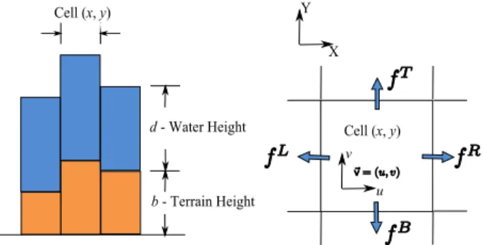
The proposed hydraulic erosion model is decomposed into five steps. Before going into the model, we first describe the necessary quantities and notations for the simulation process (cf. Figure 2):
- terrain height b - water height d
- suspended sediment amount s
- the outflow flux f = (fL, fR, fT, fB)
- velocity vector ~v= (u, v)
These values are stored for each cell of the 2D grid and kept up-to-date during the simulation. Therefore we need several layers of 2D arrays for data storage. This layered data structure has been extensively used in previous methods [2, 21].
Figure 2. Our data structure and the neigh-boring information
1Recently, we found an anterior paper by Maes et al [18] that has im-plemented an improved pipe model on GPU in a similar way. They focus on fluid simulation and incorporate a particle system (CPU-GPU mixed implementation) to handle breaking waves. We focus on extending this model to simulate the erosion process. We also present more details about the GPU implementation of the pipe model, especially about the scaling process and the limitations, which are not covered in their paper.
The five steps of our simulation are:
1. Water increases due to rainfall or river sources. 2. Flow is simulated with the shallow-water model. Then
the velocity field and the water surface are updated. 3. Erosion-deposition process is computed with the
ve-locity field.
4. Suspended sediment is transported by the velocity field.
5. Water decreases due to evaporation.
The simulation process iterates over the five steps to get gradually changing results. Each step of the simulation takes in data from previous steps and updates these values using their governing equations. Let bt, dt, st, ftand ~vtbe
the data at given time t, ∆t be the iteration time step, we
describe how to update these grid values for the time t+ ∆t
within the five steps. Since some of the data are updated in two or three steps, we use subscripts1, 2, 3... to distinguish
the intermediate updated value from the final data used for next iteration, such as dt (water height at time t), d1, d2
(intermediate water height) and dt+∆t(final water height at t+ ∆t).
3.1. Water Increment
New water appears on the terrain due to two major ef-fects: rainfall and river sources. For both types, we need to specify the location, the radius and the water intensity (the amount of water arriving during∆t). For river sources, the
location of the sources is fixed. For rainfall, each raindrop falls down on the terrain with a random distribution. Let
rt(x, y) be the water arriving at cell (x, y) per time unit,
water height is updated by a simple addition:
d1(x, y) = dt(x, y) + ∆t · rt(x, y) (1) Note that d1is an intermediate water height, which will be
changed in the following steps.
3.2. Flow Simulation
We first describe how to compute the outflow flux f based on the pipe model, and then update the water surface
d and the velocity field ~v with f .
3.2.1 Outflow Flux Computation
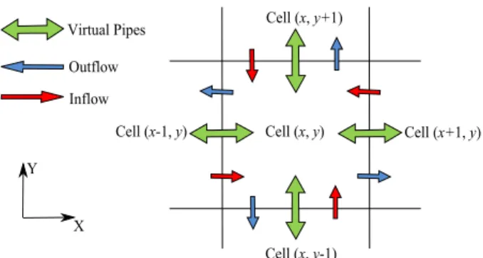
As stated in the related work, we adapt the pipe model from [22] to simulate the water movement. In the pipe model, cell
(x, y) exchanges water with its neighboring cells through
Figure 3. Pipe model notations. Each cell is connected to its four neighbors through vir-tual pipes.
pipe. To avoid confusion with the velocity field ~v, we use
the term ”flux” instead of flow velocity. At each step, the flux is accelerated by the hydrostatic pressure difference be-tween the two cells connected by the pipe. Then the wa-ter height in cell(x, y) is updated by accumulating all the
flux values from all the virtual pipes. If the updated water height is negative, all pipes that are removing fluid from the cell collect some water back from neighbors. However, this scaling back process can not be easily mapped to GPU be-cause dependent data processing on the 2D grid is involved in the process, which is not affordable on GPU.
We solve this issue by limiting the outflow flux from one cell with its water amount. We store for each cell only the outflow flux value f = (fL, fR, fT, fB), as shown in
Fig-ure 3. fLis the outflow flux from cell(x, y) to its left
neigh-bor(x − 1, y), and fR, fT, fBare defined similarly. If the
sum of the outflow flux exceeds the water amount of the cell, f will be scaled down by a factor K to avoid negative updated water height.
We calculate fLfor cell(x, y) as follows: ft+∆t(x, y) = max(0, fL tL(x, y) + ∆t · A ·
g· ∆hL(x, y)
l )
(2) where A is the cross-sectional area of the pipe, g is the ac-celeration due to gravity, l is the length of the virtual pipe, and∆hL(x, y) is the height difference between cell (x, y)
and its left neighbor(x − 1, y): ∆hL
t(x, y) = bt(x, y)+d1(x, y)−bt(x−1, y)−d1(x−1, y)
(3) For detail derivation of eqn. (2), we refer the reader to O’Brien’s original paper [22]. fR, fT, fB are computed
in a similar way. The scaling factor K for the outflow flux is then given as:
K= min(1, d1· lXlY
(fL+ fR+ fT + fB) · ∆t) (4)
where lXand lY is the distance between grid points in the X
and Y directions. So the outflow flux f = (fL, fR, fT, fB)
is scaled by K:
ft+∆ti (x, y) = K · f i
t+∆t(x, y), i = L, R, T, B (5)
3.2.2 Water Surface and Velocity Field Update
The water height is updated with the new outflow flux field by collecting the inflow flux finfrom neighbor cells, and
sending the outflow flux fout away from the current cell.
For cell(x, y), the net volume change for the water is: ∆V (x, y) = ∆t · (Xfin−Xfout) = ∆t · (fR t+∆t(x − 1, y) + f T t+∆t(x, y − 1)+ ft+∆t(x + 1, y) + fL t+∆t(x, y + 1)B − X i=L,R,T ,B ft+∆t(x, y))i (6) The water height in each cell is then updated as:
d2(x, y) = d1(x, y) +∆V (x, y)
lXlY (7)
Next, the velocity field ~v is necessary for the
erosion-deposition model (Section 3.3) and the sediment transporta-tion (Sectransporta-tion 3.4). Only the horizontal velocity is consid-ered in our study. ~v can be easily calculated from the
out-flow flux. The average amount of water that passes through cell(x, y) per unit time in the X direction can be expressed
with eqn. (8):
∆WX= f
R(x − 1, y) − fL(x, y) + fR(x, y) − fL(x + 1, y) 2
(8) And∆WX can also be computed by the velocity compo-nent u in the X direction:
lY · ¯d· u = ∆WX (9) where ¯d= d1+d2
2 is the average water height in cell(x, y)
during the first two steps. Then ut+∆tis computed using
eqn. (8) and (9). In a similar way we get the v component of ~v in the Y direction.
For any fluid simulation method, boundary conditions should be taken into consideration. Since the flow is sim-ulated on a 2D grid, we assume no water can flow out of the grid (”no slip” boundary condition). In the pipe model, we specify the outflow flux on boundary cells to satisfy the conditions. For cells (x, 0) on the left boundary, the
out-flow flux to the left neighbor fL(x, 0) should be set to zero.
Similar rules apply for the other boundaries.
The pipe model can be seen as as an explicit method for shallow-water equations. The numerical stability of the
solution is determined by the time step ∆t. The
maxi-mum time step is restricted by various factors, such as the Reynolds number, the cell size, the boundary conditions. And the scaling step might also introduce instability to the system: if the outflow flux of one cell is scaled by the factor K, the outflow flux of its neighbors should be ad-justed correspondingly to avoid a numerical error in flow rate, which is not considered in the method. For our model, the new value of one cell is calculated from its four neigh-bors. Therefore this limitation can be approximately ex-pressed with the CFL condition:∆t · u ≤ lX,∆t · v ≤ lY. When the size of the grid increases (lX, lY decrease), we
should decrease the time step proportionally to get stable simulation results.
Although all the equations introduced in the pipe model can be easily extended to handle all the eight neighbors of the current cell, we find in practice that the four von Neu-mann neighbors can produce satisfactory results.
With the updated velocity field, we proceed in the fol-lowing steps.
3.3. Erosion and Deposition
When water flows over the terrain, some soil will be eroded and transported by the water, and some suspended sediment will be deposited on the ground. This erosion-deposition process is mostly determined by the sediment transport capacity of the flow [9]. This quantity is restricted by many factors, and many prediction models have been proposed in soil science. We employ a simplified empirical equation from [12] to simulate the process. The sediment transport capacity C for the water flow in the cell(x, y) is
calculated as:
C(x, y) = Kc· sin(α(x, y)) · |~v(x, y)| (10) where Kcis a sediment capacity constant, α(x, y) is the
lo-cal tilt angle and ~v is the velocity value. From eqn. (10),
we can see that C is related to the terrain geometry and the flow velocity. Note that there is one limitation about the computation of C: for very flat terrains where the α value approaches zero, C will be very small, which means the wa-ter flow will pick up very little soil from the ground and the erosion effect is indistinctive. This problem can be allevi-ated by limiting the α value with a user-specified minimum threshold. Then we compare C with the suspended sedi-ment amount s to decide the erosion-deposition process. If
C > st, some soil is dissolved into the water and added to the suspended sediment:
bt+∆t= bt− Ks(C − st) (11a)
s1= st+ Ks(C − st) (11b)
where Ksis a dissolving constant. If C ≤ st, some
sus-pended sediment is deposited:
bt+∆t= bt+ Kd(st− C) (12a)
s1= st− Kd(st− C) (12b) where Kdis a deposition constant. The amount of the
sus-pended sediment s1will be updated again in the
transporta-tion step.
3.4. Sediment Transportation
After the erosion-deposition step, the updated suspended sediment is transported with the flow velocity field ~v. This
process can be described with the advection equation:
∂s
∂t + (~v · ∇s) = 0 (13)
We use the semi-Lagrangian advection method introduced to graphics by Stam [26] to solve the advection equation. We determine the new value for the current cell(x, y) with
the velocity field by taking an Euler step backward in time:
st+∆t(x, y) = s1(x − u · ∆t, y − v · ∆t) (14) If the position(x − u · ∆t, y − v · ∆t) is not on the grid,
we get the s value by using interpolation of the four nearest neighbors. Since the semi-Lagrangian approach is uncon-ditionally stable, there will be no stability problem for this step.
3.5. Evaporation
Finally, some water are evaporated into the air due to the environmental temperature. We assume the temperature to be constant during the simulation. And the evaporation model can be represented as:
dt+∆t(x, y) = d2(x, y) · (1 − Ke· ∆t) (15) where Keis an evaporation constant.
After the evaporation step, we get all the data at time
t+ ∆t, which is used for the next iteration. We present a
compact summary of all the steps as follows: 1. d1← W aterIncrement(dt);
2. (d2, ft+∆t, ~vt+∆t) ← F lowSimulation(d1, bt, ft);
3. (bt+∆t, s1) ← ErosionDeposition(~vt+∆t, bt, st);
4. st+∆t← SedimentT ransport(s1, ~vt+∆t);
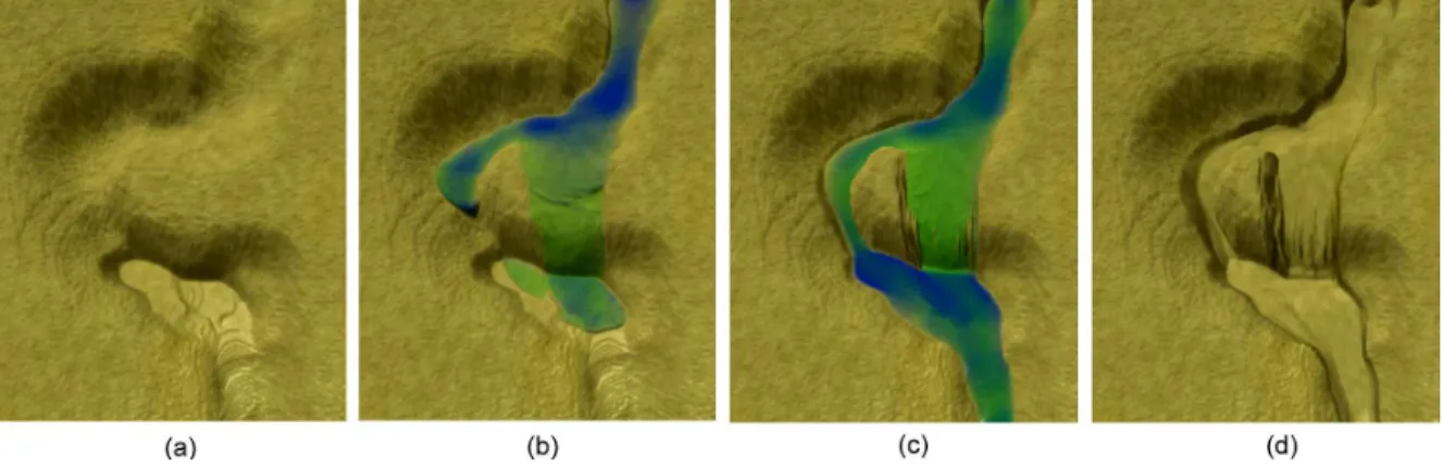
Figure 4. Water flow erodes the riverbed (b) and creates a new path (c, d).
Figure 5. Erosion and deposition in a basin (b). Center of the basin is flattened by the cumulated sediment (red) after the evaporation (c).
4. Simulation and Visualization on GPU
Harris [11] provided a basic framework for GPGPU pro-grams. The input arrays are packed into 2D textures and sent to the GPU memory. Then a quad is drawn oriented parallel to the image plane. For each pixel in the quad, a fragment is generated by the hardware rasterizer and pro-cessed by a customized fragment shader. The fragment shader takes care of the computation for each pixel, which is the kernel of the process. Finally, the output values are written into a texture or a render target, which can be used for the computation in the next pass. Complex GPGPU programs may need many passes through the pipeline to get the final results. Since fragment processors are highly paralleled and optimized, the computation is usually much faster than an equivalent CPU implementation, and scales well with the grid resolution. Furthermore, there is no need to transfer data between the host memory and the graphics memory, which is especially suitable for our simulation and visualization work.We first pack all the basic quantities into three 2D tex-tures: b, d, and s are stored in different channels of one
texture T1, f has four components, therefore stored in one
independent texture T2, and the velocity field ~v in texture T3. Following the steps described in Section 3, we imple-ment the model as a multi-pass process on GPU: For step
1, 3, 4 and 5, only one pass is needed respectively. For step 2, we should first update the outflow flux in T2, then update the water height in T1and the velocity field in T3, so three
passes are necessary. In total seven passes are needed for the simulation.
As described in the pipe model, the boundary cells re-quire separate treatment from the interior cells of the grid. Harris [10] suggested using a boundary fragment program and rendering line primitives over the edges of the viewport. We avoid this extra draw call by judging in the fragment shader whether the cell being processed is on the boundary or not. Since the flow control statements have lower penal-ties on the latest GPUs and only short branches are needed for the judgement, the unnecessary fragment operations on interior cells do not exhibit obvious performance loss in our experiments.
After the data is updated by the simulation process, the data texture T1(containing terrain and water height) can be
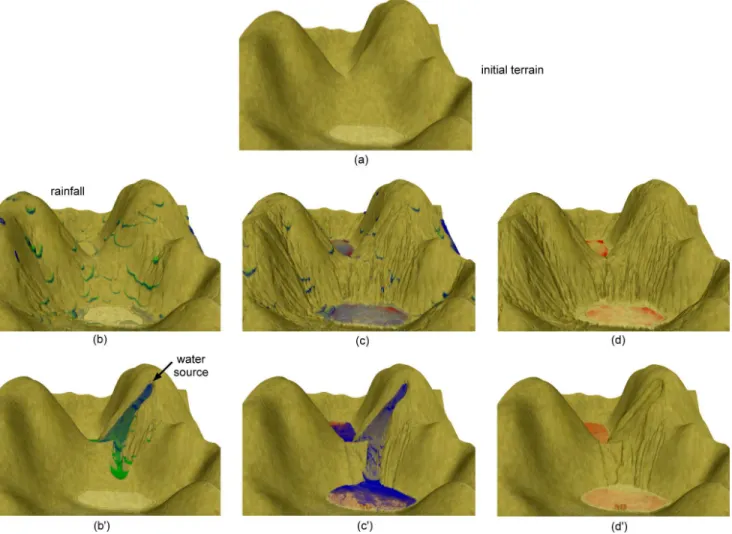
Figure 6. Mountain eroded by rainfall (b, c, d) and water source (b’, c’, d’) respectively.
used directly for the visualization. T1is sent to the vertex
shader as a vertex texture to displace the height of a prede-fined grid mesh. For efficiency reasons we draw only one height field for the whole scene, which combines the terrain and the water surfaces. The height displacement h for grid cell(x, y) is given as h(x, y) = b(x, y) + d(x, y), which is
easily obtained with one texture fetch from T1. Then a
frag-ment shader computes the final color for the cell. To get the diffuse color, the water color is blended with the terrain color; its transparency varies with the water height d. Phong lighting model is employed for per pixel lighting. Different specular coefficients are used for terrain and water surfaces respectively.
5. Experimental Results
We present the experimental results and the perfor-mances. The test platform is a Pentium IV 2.40GHz PC equipped with a nVIDIA GeForce 8800 GTX
graph-ics card. Although the experiments were run on a Di-rectX10 class graphics card, our algorithm can be imple-mented on any Shader Model 3.0 GPUs, since no Di-rectX10 features were used in the implementation. For all the examples, we use the color green to indicate the amount of the suspended sediment in the water flow, and color red for the amount of the deposited sediment on the ground, which helps us to get a better view of the im-portant features in the simulation process, such as ero-sion, deposition and sediment transportation. See video at http://evasion.imag.fr/Publications/2007/MDH07.
The first test scene is a dry river channel on a slope. A water source is put into the channel at an upriver position. A detailed view of the channel during the simulation is pre-sented in Figure 4 and the accompanying video shows the running simulation (sequence 2). Some water follows the channel, eroding the original riverbed. Some water flows out of the channel and erodes part of the river bank, cre-ating a new path for the subsequent downward flow. The eroded soil enters the suspended sediment layer, and gets
Figure 7. An erosion process that combines the rainfall and a river source.
transported by the water flow. This phenomenon is widely observed in nature.
Erosion effect by rainfall on an artificial height field has been illustrated in Figure 1. We provide another example in Figure 5 to show the effect of the deposition process. The test scene is an artificial basin. Four slopes intersect at the bottom of the basin. Rainfall brings soil down from all four slopes and deposits it at the bottom. After plenty of rainfall and the evaporation process, the slopes are highly eroded and the bottom is flattened by the cumulated sediment (de-noted in red, cf Figure 5 (c)).
Next we show in Figure 6 a mountain scene which is eroded by rainfall and a fixed river source respectively. The initial terrain is smooth. Rainfall creates interesting gullies on the hillsides, while the fixed source creates a stream bed
along the flow directions. In both cases, water and the de-posited sediment are accumulated at the bottom, forming two lakes.
A final example which combines the rainfall and a river source in one simulation process is given in Figure 7. Dif-ferent patterns created by rainfall and the river source, and all the important features for the erosion process can be ob-served in this example. The accompanying video records the dynamic simulation processes for all the examples pre-sented in this section.
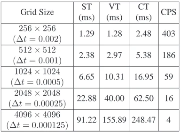
The performances of our algorithm are presented in Ta-ble 1. We define one cycle to be one simulation process plus one visualization process. For each cycle, we record the Simulation Time (ST for short, measured in millisec-onds), Visualization Time (VT, in millisecmillisec-onds), and Cycle
Grid Size ST (ms) VT (ms) CT (ms) CPS 256 × 256 (∆t = 0.002) 1.29 1.28 2.48 403 512 × 512 (∆t = 0.001) 2.38 2.97 5.38 186 1024 × 1024 (∆t = 0.0005) 6.65 10.31 16.95 59 2048 × 2048 (∆t = 0.00025) 22.88 40.00 62.50 16 4096 × 4096 (∆t = 0.000125) 91.22 155.89 248.47 4
Table 1. Performance results for different grid sizes. ST: average simulation time, VT: avg. visualization time, CT: avg. cycle time (1 cy-cle = 1 simulation + 1 visualization), CPS: avg. number of cycles per second.
Time (CT, in milliseconds). CT is also used to provide the CPS (cycles per second). As the computation cost is mostly determined by the grid size, all the examples produce sim-ilar performance results. So we only provide the results for the final mountain example in Figure 7. The grid size varies from256 × 256 to 4096 × 4096. From Table 1, we
can see that our algorithm runs interactively even on a large
2048 × 2048 size mountain. Both the simulation process
and the visualization process scale well with the changing grid size. The time cost varies linearly with the number of the cells (plus some slight overhead at the low end), which is coherent with the algorithmic complexity of the method. For grid size larger than512×512, the visualization process
occupies most of the execution time. This is due to the large number of texture fetches in vertex shader (one fetch for each cell). There is still room for further improvement: the simulation stage and the visualization stage are independent of each other, and the grid size for each stage can be differ-ent, especially for large size terrains up to4096 × 4096. We
can iterate over the simulation process for more than once before each visualization. The grid size for the visualization step can be smaller than the simulation size and the details of the terrain appearance are to be enhanced with normal maps.
6. Conclusions and Future Work
We have presented an efficient method for fast hydraulic erosion simulation and visualization. Relying on a well adapted shallow water model, our method produces real-istic eroded terrains in a physically based way. The pro-posed method also has the good property of independent
data processing, which allows its efficient implementation as a multi-pass process on GPU. We can handle large size terrains and view the erosion process at interactive rates, which are usually difficult for previous techniques. How-ever there are still sHow-everal problems to be further studied about our method: as mentioned in Section 3, the erosion model we employed has some difficulties in simulating the erosion process on very flat terrains or terrains with caves. The stability of the systems is restricted by the time step and the scaling process of the fluid solver.
As a future work, based on this method, we would like to develop an interactive system which allows terrain de-signers to edit the terrain surface, the water sources and the physical parameters interactively and see the feedback in real time. We would also like to include other erosive processes in our algorithm, such as thermal weathering and wind erosion. Simulating the erosion effects on non-height-field objects is also an interesting topic we would like to explore in the future.
Acknowledgements
The authors would like to thank Jamie Wither for proof-reading. We would also like to thank the anonymous re-viewers for their valuable comments. Xing Mei is supported by LIAMA NSFC 60073007 and by a grant from the Euro-pean Community under the Marie-Curie project VISITOR MEST-CT-2004-8270. Philippe Decaudin is supported by a grant from the European Community under the Marie-Curie project REVPE MOIF-CT-2006-22230.
References
[1] B. Bene˘s. Real-time erosion using shallow water simulation. In VRIPHYS’07: 4th Workshop in Virtual Reality Interac-tions and Physical Simulation, 2007.
[2] B. Bene˘s and R. Forsbach. Visual simulation of hydraulic erosion. Journal of WSCG, 10:79–86, 2002.
[3] B. Bene˘s, V. T˘e˘s´ınsk´y, J. Horny˘s, and S. K. Bhatia. Hy-draulic erosion. Computer Animation and Virtual Worlds, 17(2):99–108, 2006.
[4] N. Chiba, K. Muraoka, and K. Fujita. An erosion model based on velocity fields for the visual simulation of moun-tain scenery. Journal of Visualization and Computer Anima-tion, 9(4):185–194, 1998.
[5] O. Deussen and B. Lintermann. Digital Design of Nature. Springer, Berlin, Germany, 2005.
[6] J. Dorsey, A. Edelman, H. W. Jensen, J. Legakis, and H. K. Pedersen. Modeling and rendering of weathered stone. In SIGGRAPH ’99: Proceedings of the 26th annual conference on Computer graphics and interactive techniques, pages 225–234, 1999.
[7] J. Dorsey, H. K. Pedersen, and P. Hanrahan. Flow and changes in appearance. In SIGGRAPH’96: Proceedings of
the 23th annual conference on computer graphics and inter-active techniques, pages 411–420, 1996.
[8] D. Ebert, K. Musgrave, P. Peachey, K. Perlin, and S. Worley. Texturing and Modeling: A Procedural Approach. Morgan Kaufmann Publishers, San Francisco, USA, 2003.
[9] R. S. Harmon and W. W. Doe III. Landscape Erosion and Evolution Modeling. Kluwer Academic/Plenum Publishers, New York, USA, 2001.
[10] M. Harris. Fast fluid dynamics simulation on the gpu. In GPU Gems, chapter 38, pages 637–666. Addison-Wesley Professional, 2004.
[11] M. Harris. Mapping computational concepts to gpus. In GPU Gems 2, chapter 31, pages 493–508. Addison-Wesley Professional, 2005.
[12] P. Y. Julien and D. B. Simons. Sediment transport capacity of overland flow. Transactions of the ASAE, 28(3):755–762, 1985.
[13] M. Kass and G. Miller. Rapid, stable fluid dynamics for computer graphics. In SIGGRAPH ’90: Proceedings of the 17th annual conference on Computer graphics and interac-tive techniques, pages 49–57, 1990.
[14] A. D. Kelly, M. C. Malin, and G. M. Nielson. Terrain sim-ulation using a model of stream erosion. In SIGGRAPH’88: Proceedings of the 15th annual conference on computer graphics and interactive techniques, pages 263–268, 1988. [15] W. Li, X. Wei, and A. Kaufman. Implementing lattice
boltz-mann computation on graphics hardware. The Visual Com-puter, 19(7-8):444–456, 2003.
[16] Y. Liu, X. Liu, and E. Wu. Real-time 3d fluid simulation on gpu with complex obstacles. In Proceedings of Pacific Graphics’04, pages 247–256, 2004.
[17] Y. Liu, H. Zhu, X. Liu, and E. Wu. Real-time simulation of physically based on-surface flow. The Visual Computer, 21(8-10):727–734, 2005.
[18] M. M. Maes, T. Fujimoto, and N. Chiba. Efficient anima-tion of water flow on irregular terrains. In GRAPHITE ’06: Proceedings of the 4th international conference on Com-puter graphics and interactive techniques in Australasia and Southeast Asia, pages 107–115, 2006.
[19] F. K. Musgrave, C. E. Klob, and R. S. Mace. The synthesis and rendering of eroded fractal terrains. In SIGGRAPH’89: Proceedings of the 16th annual conference on computer graphics and interactive techniques, pages 41–50, 1989. [20] K. Nagashima. Computer generation of eroded valley and
mountain terrains. The Visual Computer, 13(9-10):456–464, 1998.
[21] B. Neidhold, M. Wacker, and O. Deussen. Interative phys-ically based fluid and erosion simulation. In Eurographics Workshop on Natural Phenomena’05, pages 25–32, 2005. [22] J. O’Brien and J. K. Hodgins. Dynamic simulation of
splash-ing fluids. In Proceedsplash-ings of Computer Animation’95, pages 198–205, 1995.
[23] J. D. Owens, D. Luebke, N. Govindaraju, M. Harris, J. Kruger, A. E. Lefohn, and T. J. Purcell. A survey of general-purpose computation on graphics hardware. Com-puter Graphics Forum, 26(1):80–113, 2007.
[24] P. Prusinkiewicz and M. Hammel. A fractal model of moun-tains with rivers. In Proceedings of Graphics Interface’93, pages 128–137, 1993.
[25] P. Roudier, B. Peroche, and M. Perrin. Landscapes synthesis achieved through erosion and deposition process simulation. Computer Graphics Forum, 12(3):375–383, 1993.
[26] J. Stam. Stable fluids. In SIGGRAPH ’99: Proceedings of the 26th annual conference on Computer graphics and interactive techniques, pages 121–128, 1999.
[27] B. Sutherland and J. Keyser. Particle-based enhancement of terrain data. In Siggraph’06 Research Poster, page 96, 2006. [28] G. Valette, S. Pr´evost, L. Lucas, and J. L´eonard. Soda project: A simulation of soil surface degradation by rainfall. Computer&Graphics, 30(4):494–506, 2006.
[29] E. Wu, Y. Liu, and X. Liu. An improved study of real-time fluid simulation on gpu. Journal of Computer Animation and Virtual World, 15(3-4):139–146, 2004.