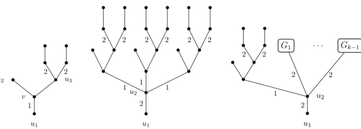
Neighbour-Sum-2-Distinguishing Edge-Weightings: Doubling the 1-2-3 Conjecture
Texte intégral
Figure
Documents relatifs
[r]
a) Déterminer par maximisation de l’hamiltonien, l’expression de la commande optimale u pour β=1. b) Montrer que seule la solution positive de l’équation de Riccati
In this paper, we consider the total graphs of the complete bipartite graphs and provide exact value for their λ-numbers.. AMS 2000 Subject Classification:
Pour rappel : Voici le tableau donnant les tables d’addition utiles pour poser une addition. (qui sont donc à
Complète les carrés magiques pour que toutes les lignes, toutes les colonnes et toutes les diagonales obtiennent la
Si c’est correct, le joueur peut avancer du nombre de cases indiqué sur le dé de la carte. Sinon, il reste à
Les élèves disposent d’un paquet de cartes et d’un plateau de jeu A3.. Le jeu nécessite aussi un dé et
Par comparaison entre ce qui est pareil et ce qui est différent, le binôme trouve ce qu’il faut donner à Minibille pour qu’elle ait autant que Maxibille.. Le
