HAL Id: hal-02466815
https://hal.inria.fr/hal-02466815
Submitted on 4 Feb 2020HAL is a multi-disciplinary open access
archive for the deposit and dissemination of sci-entific research documents, whether they are pub-lished or not. The documents may come from teaching and research institutions in France or abroad, or from public or private research centers.
L’archive ouverte pluridisciplinaire HAL, est destinée au dépôt et à la diffusion de documents scientifiques de niveau recherche, publiés ou non, émanant des établissements d’enseignement et de recherche français ou étrangers, des laboratoires publics ou privés.
On Vision-based Kinematic Calibration of a
Stewart-Gough Platform
Pierre Renaud, Nicolas Andreff, Grigoré Gogu, Philippe Martinet
To cite this version:
Pierre Renaud, Nicolas Andreff, Grigoré Gogu, Philippe Martinet. On Vision-based Kinematic Cali-bration of a Stewart-Gough Platform. IFTOMM World Congress in Mechanism and Machine Science, IFTOMM’03, pp. 1906-1911, Chine, delayed in April 2004, Apr 2004, Tianjin, China. �hal-02466815�
On Vision-based Kinematic Calibration of a Stewart-Gough Platform
Pierre Renaud, Nicolas Andreff, Grigore GoguLaboratoire de Recherche et Applications en Mécanique Avancée, IFMA – Univ. B. Pascal, 63175 Aubière, France e-mail: renaud@ifma.fr
Philippe Martinet
LAboratoire des Sciences et Matériaux pour l’Electronique et d’Automatique, Univ. B. Pascal – CNRS, 63175 Aubière, France
Abstract: In this article, we propose a vision-based kinematic calibration algorithm for Stewart-Gough parallel structures. Information on the position and orientation of the mechanism legs is extracted from the observation of these kinematic elements with a standard camera. No workspace limitation, nor installation of additional proprioceptive sensors are required. The algorithm is composed of two steps: the first one enables us to calibrate the position of the joint centers linked to the base and possibly evaluate the presence of joint clearances. The kinematic parameters associated to the moving elements of the platform are calibrated in a second step. The algorithm is first detailed, then an experimental evaluation of the measurement noise is performed, before giving simulation results. The algorithm performance is then discussed.
Keywords: Robot calibration, Parallel mechanism, Computer Vision, Lines, Plücker coordinates
1 Introduction
Compared to serial mechanisms, parallel structures exhibit a much better repeatability [1], but not better accuracy [2]. A kinematic calibration is thus also needed. The algorithms proposed to conduct calibration for these structures can be classified in three categories: methods based on the direct use of a kinematic model, on the use of kinematic constraints on mechanism parts, and methods relying on the use of redundant proprioceptive sensors.
The direct kinematic model can rarely be expressed analytically [1]. The use of numerical models to achieve kinematic calibration may consequently lead to numerical difficulties [3]. On the other hand, the inverse kinematic model can usually easily be derived analytically. Calibration can then be performed by comparing the measured joint variables and their corresponding values estimated from an end-effector pose measurement and the inverse kinematic model. The main limitation is the necessary full-pose measurement. Among the proposed measuring devices [7-10], only a few have been used to conduct parallel structure calibration [11-14]. The systems are either very expensive, tedious to use or have a low working volume. The use of an exteroceptive sensor may also lead to identifiability problems during the calibration process [15].
Methods based on kinematic constraints of the end-effector [3] or legs of the mechanism [3-6] are interesting because no additional measurement device is needed. However, the methods based on kinematic constraints of the end-effector are not numerically efficient [3], because
of the workspace restriction, and kinematic constraints of the legs of the mechanism in position or orientation seem difficult to achieve experimentally on large structures. The use of additional proprioceptive sensors on the passive joints of the mechanism enables one to have a unique solution to the direct kinematic model [16], and then use a criterion based on this model. An alternate way is to use the additional sensors on some legs to express a direct or inverse kinematic model as a function of the parameters of these legs and the redundant information. Calibration can then be achieved in a single process [17-18] or in two steps [3]. The main advantages of these methods are the absence of workspace limitation and the analytical expression of the identification criterion. However, practically speaking, the design of the mechanism has to take into account the use of these sensors. Furthermore, for some mechanisms, the passive joints can not be equipped with additional sensors, for instance spherical joints. Consequently, we propose a method that combines the advantage of information redundancy on the legs with non-contact measurements to perform the kinematic calibration.
The parallel mechanisms are designed with slim, often cylindrical, legs that link the end-effector and the base. The kinematic behavior of the mechanism is closely bound to the movement of these legs. Hence the study of their geometry has already led to singularity analysis based on line geometry [19]. For such geometrical entities, the image obtained with a camera can be bound to their position and orientation. By observing simultaneously several legs, it is then possible to get information on the relative position of the legs. Calibration can then be achieved by deriving an identification algorithm adapted to this information. No workspace limitation is introduced, nor modification of the mechanism.
In this article, we introduce an algorithm for vision-based kinematic calibration of parallel mechanisms that uses observation of the mechanism legs. The method is developed in the context of the Sewart-Gough platform [20] calibration. The method is composed of two steps: the first one consists of determining the location of the joints between the base and the legs, with the ability to analyze presence of joint clearances. The second step enables one to perform the identification of the actuator offsets and the location of the joints between the legs and the end-effector.
The first section presents the mechanism modelling. The identification algorithm is then detailed, recalling first
the relation between position and orientation of a cylindrical axis and its image projection. The two steps of the identification are then detailed. In the third section, an evaluation of the proposed method is achieved by an experimental estimation of the measurement accuracy and a simulation of the identification of a Deltalab Stewart-Gough platform. In order to discuss the calibration method, the results are analysed in terms of kinematic parameter knowledge improvement and accuracy improvement. Conclusions are then finally given on the performance and further developments of this method.
2 Kinematic Modelling
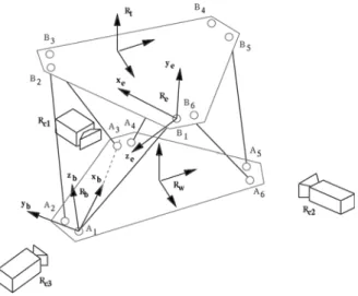
The Stewart-Gough platform is a six degree of freedom fully parallel mechanism, with six actuated legs positioning the end-effector (Fig. 1). The analysis influence of the manufacturing tolerances on the accuracy of such mechanisms has shown [2] that the most influential kinematic parameters are the position of each leg on the base and on the end-effector as well as the joint encoder offsets. Therefore 42 parameters define the kinematic model.
For manipulators, the controlled pose is the transformation between the world frame Rw and the tool
frame Rt (Fig. 1). Noting Rb the frame defined by the
joints between the legs and the base and Re the frame
defined by the joints between effector and legs, twelve parameters define the transformations wT
b between world
and base frames, and eT
t between end-effector and tool
frames. However these transformations are dependent on the application and must be identified for each tool and relocation of the mechanism. Therefore we only consider the thirty kinematic parameters that define relatively the joint locations on the base Aj and the end-effector Bj, and
the joint offsets. The transformations wT
b and eTt can be
identified by other techniques [21-22].
Figure 1 Stewart-Gough platform and the camera, represented in three successive locations 3 Algorithm
3.1 Vision-based information extraction
3.1.1 Projection of a cylinder
We consider the relationship that can be expressed between the position and orientation of the legs of the mechanism, supposed to be cylindrical of known radius R, and their image. The image formation is represented by the pinhole model [23] and we assume that the camera is calibrated.
In such a context, a cylinder image is composed of two lines (Fig. 2), generally intersecting except if the cylinder axis is going through the center of projection. Each corresponding generating line Di, i∈[1,2] can be defined
in the camera frame Rc (C, xc, yc, zc) by its Plücker
coordinates [24] (ui,hi) with ui the unit axis direction vector and hidefined by:
CP u
hi= i× (1)
where P is an arbitrary point of Di , and × represents the
vector cross product.
Figure 2 Perspective projection of a cylinder and its outline in the sensor frame
Each generating line image can be defined by a triplet (ai,bi,ci) such that this line is defined in the sensor frame
Rs (O, xs, ys) by the relation:
(
) (
)
⎪⎩ ⎪ ⎨ ⎧ = + + = 1 0 1 2 2 2 i i i T i i i c b a y x c b a (2)Due to perspective geometry, (ai,bi,ci) and hi are
colinear, thus, provided that lines are oriented, one has: i i i T i i i b c a h h h = = ) , , ( (3)
3.1.2 Determining the cylinder axis direction from the image
Since we now consider that the projection (h1,h2)of the cylinder is known, the cylinder axis direction u can be computed by: 2 1 2 1 h h h h u × × = (4)
3.1.3 Determining the cylinder axis position from the image
Furthermore the distances between the cylinder axis and the generating lines are equal to the cylinder radius. Let
M(xM,yM,zM) be a point of the cylinder axis. As hiis computed as a unit vector, we can express the belonging of M to the axis by the two equations:
R
i T i M=ε
h ,i∈[1,2] (5) with ε1=±1, ε2=-ε1. The determination of ε1 is performed in the grayscale image by analyzing the position of the cylinder with respect to the generating line d1. As the lines
are chosen with the same orientation, ε1 and ε2 are of opposite sign. C O D1 D2 d1 d2 yC xC zC xs ys
It can be easily proved that the kernel dimension of
T 2
1 h
h ]
[ is equal to one, by decomposing M on the orthogonal basis (u,h1,u×h1) . The system (5) is therefore under-determined. The position of M can be computed in two ways:
- Since the matrix T 2
1 h
h ]
[ is singular, a singular value decomposition (SVD) can be achieved, which allows the computation of the closest point to the camera frame center MSVD (xMSVD,yMSVD,zMSVD)
- A particular point, for instance MLS(xMLS,0,zMLS) can be computed, under condition of its existence, by solving the linear system (5). A comparison of these two methods is given with the experimental results.
From the observation of one leg with a camera, it is thus possible to determine the position and orientation of its axis in the camera frame.
3.2 Static part calibration
In the following we use the information on the legs to achieve the kinematic calibration of the mechanism. The identification process is performed in two steps: in the first part, we calibrate the parameters related to the static part of the mechanism and in the second part to the moving part.
3.2.1 Joint center estimation in the camera frame
For each spherical joint j, T images of the corresponding leg are stored for different end-effector poses. The position of the joint center Aj in Rc can be computed by
expressing its belonging to the axis for the T poses:
] , 1 [ , ,k k T j k jM ×u =0 ∈ A (6)
with Mk the axis point computed from the leg image in
section 3.1 and uj,k the axis orientation.
The coordinates (xAj, yAj, zAj) are therefore estimated
from the over-determined system obtained by concatenation of the 3T equations expressed in (6). As the three equations provided by the cross product for each pose are not independent, the solution is obtained by a singular value decomposition, which enables us to compute the least-squares estimate.
Notice that, with the estimated position of the joint centers Aj, the generating line images can be computed for
each pose, and compared to the lines obtained by image detection. It is then possible to evaluate the presence of joint clearances, which is not possible with proprioceptive sensors, like rotary joint sensors.
3.2.2 Joint center estimation in the base frame
The base frame is defined by using three joint centers. The joint positions in the base frame are then given by twelve parameters.
For a given camera position defined by the camera frame Rcα , mα legs can be observed for any end-effector
pose. Let Qα be this leg set. Their corresponding position
and orientation can therefore be computed in Rcα using (6).
Using the distance invariance with frame transformation, we can compute mα(mα-1)/2 equations between joint
positions in the camera frame and the base frame:
j g Q g j b R c j g R g j− = − ,( , )∈ α, > α A A A A (7)
To perform the joint position determination in the base frame, two conditions have to be fulfilled: The number of equations has first to be greater or equal to the number of parameters to identify: 12 2 ) 1 ( 1 ≥ −
∑
= L m m α α α (8)with L the number of camera positions.
Secondly, all the legs which joint position location has to be determined have to be observed at least once.
The joint center positions in the base frame Aj are
computed by non-linear minimization of the criterion C1:
∑
∑
= ∈ > ⎥⎦ ⎤ ⎢⎣ ⎡ − − − = L j g Q g j j g Rc j g Rb C 1 2 , ) , ( 1 α α α A A A A (9)At the end of this first step, the relative positions of the joint centers between base and legs are determined, without any other assumption on the kinematics than the absence of joint clearance. This latter hypothesis can be checked during the computation of the joint centers.
If the previously outlined identifiability conditions can not be fulfilled, the use of an additive calibration board linked to the base enables one to compute for each leg its position and orientation w.r.t the camera frame and also the pose of the camera w.r.t the calibration board [25]. The gathering of the data for the different camera positions is then possible.
3.3 Moving part identification
In this second step, the joint encoder offsets are identified, and consequently the relative positions of the joints between the legs and the end-effector.
For each successive camera frame Rcα , the joint center
positions on the base and the axis orientations are now known. The position of the leg end Bj can therefore be
computed for the T poses as a function of only the offset
q0j in the camera frame:
] , 1 [ , ) ( , 0 , , q q k T c c c jR jk j jkR R k j = + + ∈ α α α A u B (10)
By expressing the conservation of the distances
j g Q g j g j−B ,( , )∈ α, > B , mα(mα-1)/2 equations can be
written. Comparing the value of these distances between two consecutive positions, an error function C2 can then
be expressed as a function of the six joint offsets ] 6 , 1 [ , 0 j∈ q j :
∑ ∑ ∑
= − = > ∈ + + ⎥⎦⎤ ⎢⎣ ⎡ − − − = L T k j gjg Q Rc k g k j R k g k j c C 1 1 1( , ) 2 , , 1 , 1 , 2 α α α α B B B B (11) with Bj,k the position of Bj for the k-th end-effector pose.The determination of the six joint offsets enables us to compute the average value of Bj−Bg and therefore the relative position of the joints on the end-effector in the end-effector frame. The computation is similar to the one
achieved to compute the joint positions on the base using (6)-(9).
Notice that an alternate way to determine the location of the joints between the end-effector and the legs could be to mount the camera on the end-effector and then follow the procedure used to calibrate the base. However, we could then not identify the joint offsets.
4 Method Evaluation
The proposed method is here validated for the Deltalab Stewart-Gough platform (Fig. 3). First the calibration conditions are detailed. Then the measurement accuracy is experimentally evaluated. The simulation of the identification process with the formerly evaluated measurement noise is then achieved. To estimate the calibration method performance, analysis of the identified parameters and accuracy improvement is eventually conducted.
Figure 3 The Stewart-Gough platform 4.1 Calibration conditions
Because of the symmetry of the mechanism (Fig. 3), three different camera positions are considered (i.e. L=3). The simultaneous observation of four legs is then sufficient:
mα=4.
4.2 Measurement accuracy
As the camera is an exteroceptive sensor, two consecutive measurements can be considered as independent. The measurement accuracy can therefore be evaluated from a set of consecutive measurements, for a constant leg position.
A 1024×768 camera with a 6mm lens is used to
acquire the images, connected to a PC via an IEEE1394 bus. Ten images are stored and averaged for each pose, in order to suppress high-frequency noise. Cylinder outline detection is achieved by means of a Canny filter [26] (Fig. 4). Lines are then computed by a least-squares method.
Six equally-spaced leg orientations are considered within the extremal values. In Table 1, the upper-bound of the estimated standard deviations of the cylinder position and orientation are listed. The orientation is described with the Euler angles (ψ,θ). The position is obtained with the two methods presented in 3.1.3.
Table 1 Upper-bound of the standard deviations
Parameter ψ θ xMLS zMLS
Est. st. dev. 0.05rad 0.06rad 0.05mm 0.1mm
Parameter xMSVD yMSVD zMSVD
Est. st. dev 0.05mm 0.70mm. 0.26mm
In this application, the position is apparently more accurately computed with the second method than with the SVD. It must be also stated that the image processing could be improved by the use of a subpixel detection filter
[23-27] and now available higher CCD resolution sensor, since the accuracy is intrinsically bound to this resolution.
Figure 4 Stewart-Gough platform image after edge detection
4.3 Simulation
4.3.1 Performance evaluation
Simulation allows one to evaluate directly the knowledge improvement of the kinematic parameter values. Let ξgti be the ground-truth value of the i-th kinematic parameter (i∈[1,30]), ξini its a priori value, based on the CAD model of the mechanism, and ξidi its identified value. We can then quantify the calibration gain by the ratio proposed in [3] between the error committed before and after calibration on each kinematic parameter:
i gt i in i gt i id i CG ξ ξ ξ ξ − − − = 1 i∈[1,30] (12) A calibration gain equal to one should be obtained.
In order to evaluate the influence of a parameter estimation error, we also compute for ten randomly chosen poses the displacement error ∆X:
id gt
X = A1B1ξ −A1B1ξ
∆ (13)
and the orientation error ∆E: ϕ θ ψ ∆ ∆ ∆ = ∆E (14)
where (∆ψ, ∆θ, ∆φ) are the Euler angles defining the difference between the end-effector orientation computed with the kinematic parameter sets ξgt and the one computed with ξid.
4.3.2 Simulation process
Fifteen end-effector poses are generated by randomly selecting configurations with extreme leg lengths. These leg lengths are corrupted with noise to simulate proprioceptive sensor measurements (uniformly distrib-uted noise, variance equal to 3µm). The leg orientation and axis points Mi are modified by addition of white noise
with standard deviation equal to those previously estimated in Table 1. For each end-effector pose, three images are acquired with the camera to reduce the measurement noise. Initial kinematic parameter values are obtained by addition to the model values of a uniform noise with variance equal to 2mm. The base and end-effector frames are defined using joint centers 1, 3 and 5.
4.3.3 Results
The average calibration gains, computed by 100 simulations of the calibration, are indicated in Table 2.
The figure 5 represents the ground-truth parameter values and the mean estimation errors ξidi−ξgti .
Table 2 Simulation results
Kinematic parameters Mean(CGi) (%)
xA2 ; xA3 ; xA4 ; xA5 ; xA6 88.8 ; 88.9 ; 92.2 ; 92.7 ; 93.9 yA2 ; yA4 ; yA5 ; yA6 95.2 ; 91.7 ; 93.6 ; 83.8 zA2 ; zA4 ; zA6 41.9 ; 65.2 ; 33.9 xB2 ; xB3 ; xB4 ; xB5 ; xB6 89.7 ; 93.5 ; 93.5 ; 95.0 ; 93.2 yB2 ; yB4 ; yB5 ; yB6 89.4 ; 91.4 ; 93.9 ; 94.4 zB2 ; zB4 ; zB6 63.2 ; 63.8 ; -300 i q0 i∈[1,6] 91.0 ; 97.1 ; 93.3 ; 56.3 ; 95.2 ; 83.6 0 0.2 0.4 0.6 0.8 1 1.2 -100 0 100 200 300 400 500
Figure 5 Mean estimations errors (bars) and ground-truth values (line) of the thirty parameters
A sharp improvement of the knowledge of the kinematic parameters is observed, except for the z component of the joint locations. The negative calibration gain indicates that a priori parameter value is closer to the reference value than the identified one. The parameter estimation errors are however low with an average error between 0.04mm and 1mm.
It must also be underlined that the accuracy improvement is significant with an average displacement error reduced from 1mm for the initial kinematic parameters to 0.08mm, and an orientation error reduced from 0.12rad to 0.018rad.
5 Conclusions
In this article, a vision-based calibration method for Stewart-Gough parallel structures has been proposed. Using an exteroceptive sensor, the thirty kinematic parameters of the structure are identified. No mechanical constraint nor additional proprioceptive sensor are required. The method is low-cost as standard off-the-shelf cameras are used. The experimental evaluation of measurement accuracy and the simulation results show a significant accuracy improvement. The algorithm performance can be improved by using more accurate detection algorithms, and a better selection of the end-effector poses for calibration, which will soon be implemented.
Acknowledgements
This study was jointly funded by CPER Auvergne 2001-2003 and by the CNRS-ROBEA program through the MAX project.
References
1. Merlet, J.P., Les Robots Parallèles, Hermès, 1997
2. Wang, J., Masory, O., On the accuracy of a stewart
platform – part I: the effect of manufacturing tolerances, In: Proc. of ICRA, 114-120, 1993
3. Daney, D., Etalonnage géométrique des robots parallèles. PhD Dissertation, Université de Nice – Sophia-Antipolis, 2000
4. Geng, Z., Haynes, L.S., An effective kinematics calibration method for stewart platform, In: ISRAM, 87-92, 1994 5. Zhuang, H., Roth, Z.S., Method for kinematic calibration of
stewart platforms, J. of Rob. Syst., 10(3): 391-405, 1993 6. Khalil, W., Besnard, S., Self calibration of Stewart-Gough
parallel robots without extra sensors, IEEE Trans. On Rob. And Automation, 15(16): 1116-1121, 1999
7. Curtino, J.F., Schinstock, D.E. and Prather, M.J., Three-dimensional metrology frame for precision applications, Precision Engineering, 23: 103-112
8. Vincze, M., Prenninger, J.P. and Gander, H., A laser tracking system to measure position and orientation of robot end effectors under motion, The Int. J. of Robotics Research, 13(4): 305-314, 1994
9. Masory, O., Jiahua, Y., Measurement of pose repeatability of Stewart platform, J. of Rob. Syst., 12(12): 821-832, 1995 10. Schmitz, T., Zlegert, J., A new sensor for the
micrometre-level measurement of three-dimensional dynamic contours, Meas. Science Technology, 10: 51-62, 1999
11. Zhuang, H., Masory, O., Kinematic calibration of a Stewart platform using measurements obtained by a single theodolite, In: Proc. of IEEE Conf. On Intelligent Robots and Systems, 329-334, 1995
12. Geng, Z.J., Haynes, L.S., A “3-2-1” kinematic configuration of a Stewart platform and its application to six degrees of freedom pose measurements, J. of Robotics and Computer Integrated Manufacturing, 11(1): 23-34, 1994
13. Fried, G., Djouani, K., Amirat, Y., François, C., A 3-D sensor for parallel robot calibration, A parameter Perturbation Analysis, Recent Advances in Robot Kinematics, 451-460, 1996
14. Vischer, P., Clavel, R., Kinematic calibration of the parallel delta robot, Robotica, 16:207-218, 1998
15. Renaud, P., Andreff, N., Marquet, F., Dhome, M., Vision-based kinematic calibration of a H4 parallel mechanism, ICRA 2003, to appear
16. Tancredi, L., De la simplification et la résolution du modèle géométrique direct des robots parallèles, PhD Dissertation, Ecoles des Mines de Paris, 1995
17. Wampler, C., Arai, T., Calibration of robots having kinematic closed loops using non-linear least-squares estimation, In: Proc. IFToMM-jc Int. Symp. On Theory of Machine and Mechanisms, 153-158, 1992
18. Zhuang, H., Self calibration of parallel mechanisms with a case study on Stewart platforms, IEEE Trans. On Robotics and Automation, 13(3): 387-397, 1997
19. Merlet, J.P., Parallel manipulators, Part 2, Singular Configurations and Grassmann geometry, Res. Report RR-0791T, INRIA, 1988
20. Stewart, D., A platform with six degrees of freedom, In: Proc. Instr. Mech. Engr., 180: 371-386, 1965
21. Tsai, R.Y., Lenz, R.K., A new technique for fully autonomous and efficient 3D robotics hand/eye calibration, IEEE Trans. On Rob. and Automation, 5(3): 345-358, 1989 22. Andreff, N., Horaud, R., Espiau, B., Robot hand-eye
calibration using structure-from-motion, Int. J. Robotics Research, 20(3): 228:248, 2001
23. Faugeras, O., Three-dimensional Computer Vision: A Geometric Viewpoint, The MIT Press, 1993
24. Pottmann, H., Peternell, M., Ravani,B., Approximation in line space – applications in robot kinematics and surface reconstruction, Advances in Robot Kinematics: Analysis and Control, 403-412, 1998
25. Dhome, M., Richetin, M., Lapreste, J.T., Rives, G., Determination of the attitude of 3-D objects from a single perspective view, IEEE Trans on Pattern Analysis and Machine Intelligence, 11(12): 1265-1278, 1989
Mean estimation errors (mm)
Ground-truth values (mm)
26. Canny, J.F., A computational approach to edge detection, IEEE Trans. Pattern Analysis and Machine Intelligence, 8(6): 679-698, 1986
27. Steger C., Removing the Bias from Line Detection, In CVPR97, 1997