Formally-Proven Kosaraju's algorithm

HAL Id: hal-01095533

https://hal.archives-ouvertes.fr/hal-01095533v2

HAL is a multi-disciplinary open access archive for the deposit and dissemination of sci-entific research documents, whether they are pub-lished or not. The documents may come from

L’archive ouverte pluridisciplinaire HAL, est destinée au dépôt et à la diffusion de documents scientifiques de niveau recherche, publiés ou non, émanant des établissements d’enseignement et de

Formally-Proven Kosaraju’s algorithm

Laurent Théry

To cite this version:

Formally-Proven Kosaraju’s algorithm

Laurent Th´

ery

[email protected]

Abstract

This notes explains how the Kosaraju’s algorithm that computes the strong-connected components of a directed graph has been for-malised in the Coq prover using the SSReflect extension.

1

Introduction

Our interest in this algorithm comes from an initial quest for formalising the classic 2-Sat problem : given a set S of binary clauses, checking if S is satisfiable can be done in linear time. The standard justification is to rewrite the satisfiability problem into a graph problem. The transformation is straightforward. The vertices of the graph are the variables occurring in the clauses and their negations. Two edges are created for each clause l1∨ l2:

one from ¬l1 to l2 and the other from ¬l2 to l1. These two edges correspond

to logical implications and read as “if l1 is false then l2 is true” and “if l2 is

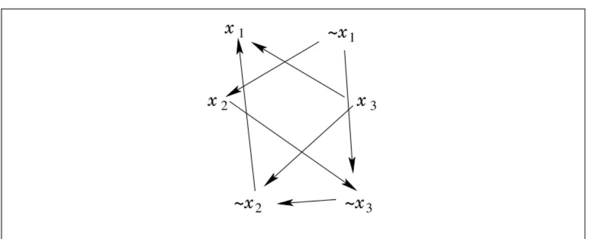
false then l1 is true” respectively. Figure1shows the graph that corresponds

to the set S = {x1∨ x2, x1∨ ¬x3, ¬x2 ∨ x3}.

Now, the claim is that the initial formula is satisfiable if and only no variable xi and its negation ¬xi both belong to the same strongly-connected

com-ponent of the resulting graph. Let us try to explain this claim informally. First, recall what a strongly-connected component is. Two vertices a and b are strongly connected if a is connected to b and b connected to a. Now, remembering the interpretation of edges as logical implications, two vertices a and b are then in the same component if the constraints given by the set of clauses force their respective truth value to be the same. In other words, if a is true, then its implication b must also be true and if b is true, then its implication a must be true. Obviously, if xi and ¬xi are in the same

~x x 3 2 ~x 1 1 x_{2 3} x _~x

Figure 1: Implication graph for the set S = {x1∨ x2, x1∨ ¬x3, ¬x2∨ x3}.

component, they cannot have both the same truth value, so the formula is unsatisfiable. A slightly more subtle argument needs to be used to show the converse. We will not explain it here.

Remember that our initial interest was in showing that 2-Sat can be solved in linear time. We are almost there. First, it is clear that the graph can be built in linear time. If there exists a linear algorithm that computes the strongly-connected components of a directed graph, then a single traver-sal of the components of the graph is sufficient to check the satisfiability of the initial set of clauses. In the literature, the algorithm for computing the strong-component of a graph is usually the one by Tarjan [4]. When trying to figure out if there were some alternatives that may lead to somewhat simpler correctness proofs, we discover the less known but beautiful Kosaraju’s algo-rithm [3]. Its formalisation is what this note is about. We will first explain the algorithm and how it can be programmed inside the Coq system. Then, we will show how a correctness proof can be derived.

2

Kosaraju’s algorithm

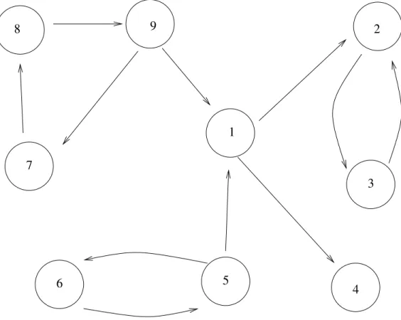
Figure 2 presents the graph we are going to use throughout this section. It is composed of 9 vertices and 11 edges. An arbitrary finite type T is used in SSReflect to represent the vertices

8 2 1 3 4 5 7 6 9

Variable T : finType.

This means that informally we have T = {1, 2, 3, 4, 5, 6, 7, 8, 9} for our exam-ple. The adjacency relation is then represented by a relation on T

Variable r : rel T .

where r x y is true if there is an edge from x to y. This means that we have r 1 2 but not r 1 5 for our example.

Now, given the relation r, in order to manipulate algorithmically the graph, we are going to use the function rgraph that computes the neighbor-hood of a vertex: rgraph r x returns the sequences of vertices that are directly connected to x. We define gr as a shortcut for our neighborhood function.

Definition gr := rgraph r.

We have for our graph gr 1 = [:: 2; 4] gr 2 = [:: 3] gr 3 = [:: 2] gr 4 = [::] gr 5 = [:: 1; 6] gr 6 = [:: 5] gr 7 = [:: 8] gr 8 = [:: 9] gr 9 = [:: 1; 7]

Kosaraju’s algorithm has two distinct phases. The first phase sorts topo-logical the vertices. This is done with a variant of the depth-first search algorithm that is already defined in the library1_.

1

We took some liberty with the actual SSReflect code. We have omitted system-atically arguments that Coq sometimes requires in order to ensure termination. There are not essential for the correctness. Also, we have used subscript to expose explicitly the parametricity of our definition over r. The last step of the algorithm requires to take a specific r

Function dfsr l x := if x ∈ l then l else foldl dfsr (x :: l) (gr x).

This definition uses the function foldl that iterates a function on elements of a list, i.e. f oldl f v [:: x1; x2; . . . xn] = f (f ( . . . f (f x1 v) x2) . . . ) xn.

The call dfsr l x starts the search at x avoiding the vertices in l and returns l

plus the vertices that have been encountered. For example, df s [::] 1 returns [:: 4; 3; 2; 1], i.e. the vertices that are connected to 1.

Unfortunately, this function does not compose very well. If we call again dfs on an unreached vertex, let’s say 5, avoiding the elements connected to 1 we get [:: 6; 5; 4; 3; 2; 1]. 5 ends up in the sequence between 1 and 6 which is problematic if we are interested by sorting topologically the graph. Of course, the problem comes from the way the vertices are collected, some kind of postfix ordering should be used. Replacing the single list l by a pair of lists fixes the problem. The first list is used to collect the vertices that need to be avoided while the other imposes a postfix order.

Function pdfsr p x :=

if x ∈ p.1 then p else

let p0 := foldl pdfsr (x :: p.1, p.2) (gr x) in (p0.1, x :: p0.2).

x is added to the first list beforehand to avoid cycling while it is added afterward for the second element to get the postfix order. Calling pdfsr ([::

], [::]) 1 returns ([:: 4; 3; 2; 1], [:: 1; 4; 2; 3]), the two list represent two different ordering of the vertices connected to 1, the second one being the one we are interested in. Now, calling pdfsr ([:: 4; 3; 2; 1], [:: 1; 4; 2; 3])

5 returns ([:: 6; 5; 4; 3; 2; 1], [:: 5; 6; 1; 4; 2; 3]). In the second list, 5 is before 1 and 6.

We actually use a slightly modified version of pdfs. As we are interested in the second sequence of the pair p only, we turn the first sequence into a set. Doing this, we just erase the irrelevant information of the ordering in which the elements of the first sequence are collected and just keep the relevant information that avoids cycling.

Function pdfsr p x :=

if x ∈ p.1 then p else

let p0 := foldl pdfsr ({x} ∪ p.1, p.2) (gr x) in (p0.1, x :: p0.2).

Getting the ordered sequence of all vertices is then done applying a foldl on the sequence of all the vertices given by the function enum

Definition stackr := (foldl pdfsr (∅, [::]) (enum T )).2.

If we suppose that enum T returns the sequence [:: 1; 2; 3; 4; 5; 6; 7; 8; 9] for our example, the value for stack is then [:: 9; 8; 7; 5; 6; 1; 4; 2; 3]. This ends the first phase of the algorithm.

The second phase is even simpler and takes advantage of the following two simple observations. First, the depth-first search function has been called on each element on the stack either at top level if the vertex was not reached yet, or by a recursive call. Second, if x connects to y but y occurs before x in sequence, we can conclude that y connects to x. This is because of the topological ordering. Suppose the call of the search at x was done at top-level with an avoiding sequences l1 generating all the connected elements

l2. The sub-sequence starting at x would be the exact concatenation of l1

and l2. This is impossible, y should occur either in l1 or in l2, so also in

the sub-sequence starting at x. This means that the call was not made at top-level and it is the depth-first search starting at y that has triggered the one at x. x is then connected to y.

Now if we take x the top of the stack, (in our example x = 9), and collect the vertices that connect to x (in our example 7, 8 and 9). What we have said before proves that this is a strongly-connected component. Two observations end the implementation of the second phase. First, computing the vertices that connect to x can be done using the same depth-first algorithm but this time applied on the graph where the edges are flipped. Second, removing the strongly-connected component of x from the stack leads to a new stack where the same process can be iterated. This iteration is implemented once again with a foldl.

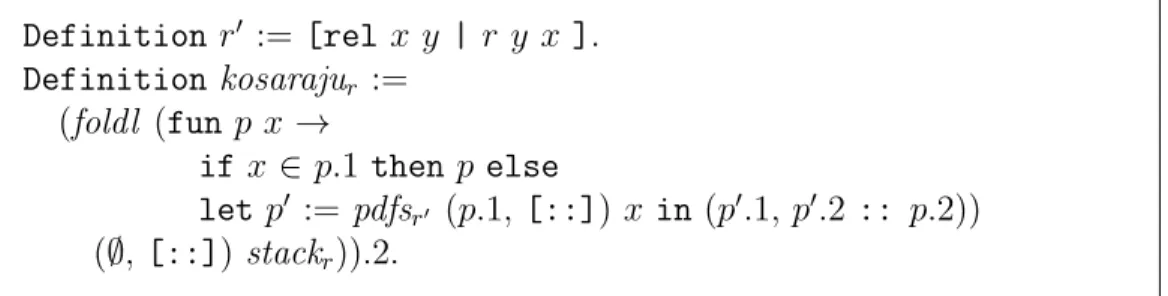
Definition r0 := [rel x y | r y x ]. Definition kosarajur := (foldl (fun p x → if x ∈ p.1 then p else let p0 := pdfsr0 (p.1, [::]) x in (p0.1, p0.2 :: p.2)) (∅, [::]) stackr)).2.

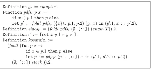
Figure 3 at page 12 collects the 11 lines of code that were necessary to implement Kosaraju’s algorithm in our functional setting. Applying it on our example gives [:: [:: 2; 3]; [:: 4]; [:: 1]; [:: 5; 6]; [:: 9; 8; 7]].

3

Correctness proof

Finding the right definitions and the intermediate results is the main diffi-culty of this proof. This is what we are going to explain in this section. We refer to the Coq source available at

http://www.sop-inria.fr/team/marelle/Laurent.Thery/Kosaraju/Kosaraju.html

for the actual proofs.

As the proof relies heavily on sequences, we first give a quick summary of the functions and predicates from the standard library we have been using in our proof.

- uniq l is true if the sequence l does not have duplicate;

- {subset l1 ≤ l2} is true if all the elements of l1 are in l2;

- l1 =i l2 is true if l1 and l2 have the same elements;

- [disjoint l1 & l2] is true if there is no common element between l1

and l2.

- nth x l n returns the nth element of the sequence. It returns x if the sequence contains less than n elements;

- [seq i ← l | P i ] returns sub-sequence of l composed of the elements of l that verify the property P ;

- flatten l returns the concatenation of all the sequences in l (l is a sequence of sequences);

- find P l returns the index of the first element of the sequence l that verifies the predicate P . It returns the size of the sequence if there is no element of l that verifies P ;

- index x l returns the index of the first occurrence of x in l. It returns the size of the sequence if x does not occur in l;

In the standard library of SSReflect, there is already the notion of being connected.

Definition x −→∗_r y := y ∈ dfsr [::] x.

A variant of it has been defined, It is the notion of being connected but with some forbidden intermediate vertices.

Definition x −→∗_r,s y :=

let r0 := [rel x y | r x y && y /∈ s ] in x −→∗ r0 y.

It is then possible to give a definition of what it is to be strongly connected

Definition x ←→∗_r,s y := x −→∗_r,s y && y −→∗_r,s y.

This is all we need for the graph path. The next step is to capture the post-fix order of our sequence. We first define the order in a sequence that is taken with respect to first occurrence

Definition x ≤r,l y := index x l ≤ index y l.

Then, we define a function that computes the canonical vertex associated to a vertex x for a pair p composed of a set and a sequence (s, l). This canonical vertex is defined as the first vertex in l that is strongly connected with x avoiding s.

Definition [x]r,p := nth x p.2 (find (fun y → x ←→∗r,p.1 y) p.2).

The central property in our proof is the notion for a pair to be well-formed. A pair (s, l) is well-formed, if s and l are disjoint and every time one takes a vertex x in l and a vertex y that is connected to x avoiding s then y is also in l and the canonical vertex of x in l avoiding s is before y in l.

Definition Wfr p :=

[disjoint p.1 & p.2] ∧

∀x y, (x ∈ p.2 ∧ x −→∗

r,p.1 y) ⇒ (y ∈ p.2 ∧ [x]r,p ≤r,p.2 y).

The disjoint part insures that the set and the sequence keep separated, the “y ∈ p.2 ” part that that the list is closed under connection and the “[x]r,p

≤r,p.2 y” part that it is in post-fix order. Intuitively, it says that canonical

elements are always on the left of the elements it connects to.

The first key property that we derive from this definition is some kind of compositionality. It indicates how well-formed pairs can be concatenated.

Lemma wf cat :

∀s1 l1 l2, Wfr (s1, l1) ⇒ Wfr (s1 ∪ {set x ∈ l1}, l2) ⇒ Wfr (s1, l2 ++ l1).

It is used to justify the computation of foldl inside the definition of the depth-first search where we accumulate the various sub-searches.

The second key property is related with the body of the pdfs and how the search starting at x can be reduced to searching at the vertices immediately connected to x. Lemma wf cons : ∀x s l, (∀y, y ∈ l ⇒ x −→∗_r,s y) ⇒ (∀y, r x y ⇒ y /∈ {x} ∪ s ⇒ y ∈ l) ⇒ x /∈ s ⇒ Wfr ({x} ∪ s, l) ⇒ Wfr (s, x :: l).

This property reads like this. Let us suppose that the pair ({x} ∪ s, l) is well-formed. In order to derive that (s, x :: l) is well-formed it is sufficient that l is composed of vertices connected to x avoiding s. Among these vertices, there must be the ones directly connected to x.

It is relatively straightforward to get the correctness of the pdfs function from the two previous properties. The statement is somewhat more intricate than expected since we also want to get the extra property that the result we get is without duplicate. Also, we need to clearly state that what is added to the second sequence is well-formed and contains only vertices connected with the initial vertex we start the search with.

Lemma pdfs correct : ∀s l x, (uniq l ∧ {subset l ≤ s}) ⇒ let (s1, l1) := pdfsr (s, l) x in if x ∈ s then (s1, l1) = (s, l) else uniq l1 ∧ ∃l2, (x ∈ l ∧ s1 = s ∪ {set x ∈ l2} ∧ l1 = l2 ++ l) ∧ (Wfr (s, l2) ∧ ∀y, y ∈ l2 ⇒ x −→∗r,s y).

Once pdfs correct is proved, the correctness of the stack can be easily derived with a simple application of wf cat. The statement of the theorem just states that the stack is well-formed and contains all the vertices.

Lemma stack correct : Wfr (∅, stackr) ∧ ∀x, x ∈ stackr.

In order to get the final correctness statement of the Kosaraju’s algorithm we just need two extra properties about well-formedness. The first one states that removing the strongly-connected component of the top element of the sequence preserves well-formedness.

Lemma wf inv :

The second one states that this strongly-connected component can be com-puted by finding the elements that connects to the top element.

Lemma wf equiv : ∀x y s l,

Wfr (s, x :: l) ⇒ (x ←→∗r,s y) = ((y ∈ x :: l) && y −→ ∗ r,s x).

With these two properties, it is almost direct to prove the correctness of Kosaraju’s algorithm. We only use notions that are present in the standard library for its statement. The result of the algorithm is a sequence of sequence l. When l is flattened, it contains every vertex once and only once and a sequence in l represents a strongly-connected component.

Lemma kosaraju correct :

(let l := flatten kosarajur in uniq l ∧ ∀x, x ∈ l) ∧

∀c, c ∈ kosarajur ⇒ ∃x, ∀y, (y ∈ c) = (x −→∗r y && y −→ ∗ r x)

Note that components are never empty since we have x −→∗_r x for all x.

4

Conclusion

Formalising Kosaraju’s algorithm has been an interesting exercise. We have chosen a direct formalisation with almost no abstraction. The key part of the formalisation has been to define the notion of well-formed pairs. It gives us a direct way to derive the correctness of the algorithm. Other formalisations of algorithms that compute strong components already exist [1, 2], we believe ours is one of the more concise.

References

[1] Peter Lammich. Verified efficient implementation of Gabow’s strongly connected component algorithm. In ITP’14, volume 8558 of LNCS, pages 325–340, 2014.

[2] Fran¸cois Pottier. Depth-first search and strong connectivity in Coq. In JFLA’15. available athttps://hal.archives-ouvertes.fr/JFLA2015.

Definition gr := rgraph r.

Function pdfsr p x :=

if x ∈ p.1 then p else

let p0 := foldl pdfsr ({x} ∪ p.1, p.2) (gr x) in (p0.1, x :: p0.2).

Definition stackr := (foldl pdfsr (∅, [::]) (enum T )).2.

Definition r0 := [rel x y | r y x ]. Definition kosarajur := (foldl (fun p x → if x ∈ p.1 then p else let p0 := pdfsr0 (p.1, [::]) x in (p0.1, p0.2 :: p.2)) (∅, [::]) stackr)).2.

Figure 3: Kosaraju’s algorithm in SSReflect

[3] Micha Sharir. A strong-connectivity algorithm and its applications in data flow analysis. Computers and Mathematics with Applications, 7:67– 72, 1981.

[4] Robert Tarjan. Depth first search and linear graph algorithms. SIAM Journal on Computing, 1972.