HAL Id: hal-00316907
https://hal.archives-ouvertes.fr/hal-00316907
Submitted on 1 Jan 2001
HAL is a multi-disciplinary open access
archive for the deposit and dissemination of
sci-entific research documents, whether they are
pub-lished or not. The documents may come from
teaching and research institutions in France or
abroad, or from public or private research centers.
L’archive ouverte pluridisciplinaire HAL, est
destinée au dépôt et à la diffusion de documents
scientifiques de niveau recherche, publiés ou non,
émanant des établissements d’enseignement et de
recherche français ou étrangers, des laboratoires
publics ou privés.
Arctic winter: 3-D simulations on the potential role of
different PSC types
J. Hendricks, F. Baier, G. Günther, B. C. Krüger, A. Ebel
To cite this version:
J. Hendricks, F. Baier, G. Günther, B. C. Krüger, A. Ebel. Stratospheric ozone depletion during
the 1995?1996 Arctic winter: 3-D simulations on the potential role of different PSC types. Annales
Geophysicae, European Geosciences Union, 2001, 19 (9), pp.1163-1181. �hal-00316907�
Geophysicae
Stratospheric ozone depletion during the 1995–1996 Arctic winter:
3-D simulations on the potential role of different PSC types
J. Hendricks1,*, F. Baier1,†, G. G ¨unther2, B. C. Kr ¨uger3, and A. Ebel1
1Institut f¨ur Geophysik und Meteorologie, Universit¨at zu K¨oln, EURAD, Aachener Str. 201-209, D-50931 K¨oln, Germany *now at: DLR, Institut f¨ur Physik der Atmosph¨are, Oberpfaffenhofen, D-82234 Weßling, Germany
†now at: DLR, Deutsches Fernerkundungsdatenzentrum, Oberpfaffenhofen, D-82234 Weßling, Germany
2Institut f¨ur Stratosph¨arische Chemie, Forschungszentrum J¨ulich, D-52425 J¨ulich, Germany
3Institut f¨ur Meteorologie und Physik, Universit¨at f¨ur Bodenkultur Wien, T¨urkenschanzstr. 18, A-1180 Wien, Austria
Received: 16 November 2000 – Revised: 13 June 2001 – Accepted: 20 June 2001
Abstract. The sensitivity of modelled ozone depletion in the
winter Arctic stratosphere to different assumptions of preva-lent PSC types and PSC formation mechanisms is investi-gated. Three-dimensional simulations of the winter 1995/96 are performed with the COlogne Model of the Middle Atmo-sphere (COMMA) by applying different PSC microphysical schemes. Model runs are carried out considering either liquid or solid PSC particles or a combined microphysical scheme. These simulations are then compared to a model run which only takes into account binary sulfate aerosols. The results obtained with the three-dimensional model agree with tra-jectory-box simulations performed in previous studies. The simulations suggest that conditions appropriate for type Ia PSC existence (T < TNAT) occur over longer periods and
cover larger areas when compared to conditions of poten-tial type Ib PSC existence. Significant differences in chlo-rine activation and ozone depletion occur between the sim-ulations including only either liquid or solid PSC particles. The largest differences, occurring over large spatial scales and during prolonged time periods, are modelled first, when the stratospheric temperatures stay below TNAT, but above
the threshold of effective liquid particle growth and second, in the case of the stratospheric temperatures remaining be-low this threshold, but not falling bebe-low the ice frost point. It can be generally concluded from the present study that dif-ferences in PSC microphysical schemes can cause significant fluctuations in ozone depletion modelled for the winter Arc-tic stratosphere.
Key words. Atmospheric composition and structure
(aerosols and particles; cloud physics and chemistry; middle atmosphere composition and chemistry)
Correspondence to: J. Hendricks
(Johannes.Hendricks@dlr.de)
1 Introduction
It is now well established that the occurrence of polar strato-spheric clouds (PSCs) in the winter polar stratosphere and the related heterogeneous chemistry can induce strong chlorine activation and subsequent ozone depletion (e.g. WMO, 1995, 1999). PSC particles can be composed of crystalline nitric acid trihydrate (NAT, Type Ia PSCs) (Hanson and Mauers-berger, 1988) or supercooled ternary H2SO4/HNO3/H2O
so-lutions (STS, Type Ib PSCs) (e.g. Carslaw et al., 1994; Tabazadeh et al., 1994). Type I PSCs can occur even above the ice frost point (Tice). At temperatures below Tice, PSC
particles consisting of water-ice (Type II PSCs) can be ob-served (e.g. Poole and McCormick, 1988). Since tempera-tures in the Arctic stratosphere fall infrequently below Tice
over prolonged time periods and large spatial scales, type I PSCs are observed much more frequently than type II PSCs during Arctic winters (e.g. Browell et al., 1990; Dye et al., 1992; Biele et al., 1998).
The rates of heterogeneous reactions on type I PSC par-ticles significantly depend on the parpar-ticles phase (Ravis-hankara and Hanson, 1996). Hence, the microphysical state of type I PSCs may influence ozone depletion rates. This further implies that stratospheric ozone loss simulated by at-mospheric chemistry models may be affected by the respec-tive concepts of PSC schemes applied. Several recent model studies were focussed on quantifying this effect. Sessler et al. (1996) performed simulations of ozone depletion in the Arctic winter stratosphere considering various PSC schemes. A chemistry-box-model was applied in that study assuming typical conditions encountered in the Arctic winter strato-sphere at 50 hPa. Additionally, a two-dimensional (2-D) chemistry-transport-model (CTM) was employed to simu-late ozone depletion on the 465 K isentropic surface dur-ing the winter 1994/95. Upper and lower limits for ozone loss were modeled when type I PSCs are considered to be composed of NAT or STS, respectively. Assuming NAT
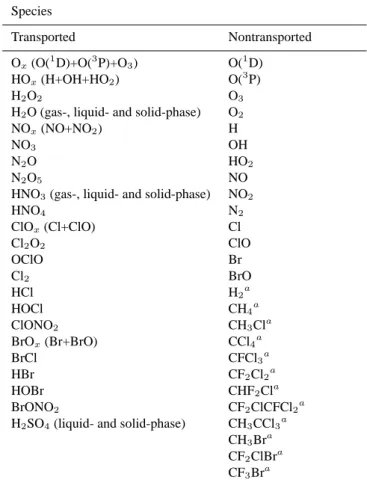
par-Table 1. Chemical constituents and families included in the model
Species
Transported Nontransported
Ox(O(1D)+O(3P)+O3) O(1D)
HOx(H+OH+HO2) O(3P)
H2O2 O3
H2O (gas-, liquid- and solid-phase) O2
NOx(NO+NO2) H
NO3 OH
N2O HO2
N2O5 NO
HNO3(gas-, liquid- and solid-phase) NO2
HNO4 N2 ClOx(Cl+ClO) Cl Cl2O2 ClO OClO Br Cl2 BrO HCl H2a HOCl CH4a ClONO2 CH3Cla BrOx(Br+BrO) CCl4a BrCl CFCl3a HBr CF2Cl2a HOBr CHF2Cla BrONO2 CF2ClCFCl2a
H2SO4(liquid- and solid-phase) CH3CCl3a
CH3Bra
CF2ClBra
CF3Bra
aConstant 2-D distribution assumed
ticles, a larger ozone decline is simulated than in the case of STS. Differences in ozone mixing ratio modelled for the late winter range between 0.1 and 0.5 ppmv in the performed simulations. Br¨uhl et al. (1997) used a trajectory-box-model to simulate stratospheric ozone loss over the Arctic during the four winters from 1992/93 to 1995/96. Similar to the work of Sessler et al. (1996), respective simulations consid-ering type I PSCs to be solid or liquid were compared in that study. Differences in the modelled late winter ozone mixing ratio of 0.1-0.2 ppmv on the 425 to 465 K isentropic levels were simulated. In contrast to the results of Sessler et al. (1996), during the winter 1994/95 simulation, liquid PSC particles induced the largest ozone loss. The results of Br¨uhl et al. (1997) agree well with trajectory calculations by Carslaw et al. (1997). Potential reasons for the discrepan-cies in the sign of the PSC scheme effect occurring between the work of Sessler et al. (1996) and the two other studies are differences in uptake coefficients of heterogeneous reac-tions on NAT and deviareac-tions in NAT formation thresholds which may significantly impact modelled ozone depletion (Carslaw et al., 1997). Massie et al. (2000) performed 3-D simulations on the chemistry of the Arctic stratosphere dur-ing the winter 1995/96. They focussed on chlorine activa-tion in December 1995 and early January 1996. Employing different microphysical schemes, they modelled significant
differences in active chlorine concentrations within the polar vortex. The study suggests that chlorine activation simulated for early winter 1995/96 is larger when NAT particle for-mation is taken into account compared to simulations where only liquid particles are considered.
The findings of the previous studies indicate that differ-ences in the PSC schemes applied in stratospheric chem-istry models can cause significant variations in the ozone concentration simulated for the Arctic winter lower strato-sphere. For late winter/early spring, when ozone depletion is the strongest, maximum differences in ozone concentra-tion of around 20% are simulated. However, since exchange with ambient air masses is not represented in the trajectory and box calculations and vertical diabatic mass exchange is neglected in the 2-D CTM simulations, it remains unclear whether these results are transferable to 3-D model calcu-lations. (In the work of Massie et al. (2000), ozone deple-tion is not considered). Hence the objective of the present study is to reinvestigate the effect of different concepts of PSC schemes on modelled ozone depletion by means of 3-D calculations. Simulations were performed with the COlogne Model of the Middle Atmosphere (COMMA) employing a NAT, an STS and a more comprehensive PSC scheme which allows the freezing of STS particles. The model calculations were carried out for the Arctic winter 1995/96 which was characterized by very low stratospheric temperatures and a strong ozone decline over the polar region and northern Eu-rope.
The next section provides a model description and an il-lustration of the different PSC schemes employed. In Sect. 3, the methodology of this study is explained. Furthermore, the results are presented and discussed. The main conclusions are drawn in Sect. 4.
2 Model description
2.1 The dynamical module
The COMMA dynamical module was developed from the global mechanistic model of the middle atmosphere formu-lated by Rose (1983). An early version of the module in-cluding the lower thermosphere was described by Jakobs et al. (1986). The module solves the primitive dynamical equations on a Eulerian grid for the altitude range from the surface up to a 150 km altitude. The model atmosphere is driven by explicitly calculated heating and cooling rates due to solar and terrestrial radiation, as described by Dameris et al. (1991) and Berger and Dameris (1993). Time ten-dencies of horizontal momentum and temperature fields are integrated using a diffusive leap-frog scheme (Haltiner and Williams, 1980). In order to guarantee Courant stability, a zonal Fourier filter is applied to the prognostic variables at high latitudes (Holloway et al., 1973). Model physics in-cludes a first order approximation of gravity wave drag us-ing generalized Rayleigh friction in the functional form de-scribed by Schoeberl and Strobel (1978). For a detailed
description of the COMMA dynamical module, its vali-dation and application, see Dameris et al. (1991), Berger and Dameris (1993), Berger and Ebel (1995), G¨unther and Dameris (1995) and Berger and von Zahn (1999).
In order to simulate the chemistry and transport of at-mospheric constituents in the lower stratosphere and tro-posphere during real winter episodes, the model-prognostic fields were replaced by interpolated 6 hourly European Cen-tre for Medium Range Weather Forecasts (ECMWF) analy-ses at all grid levels below 10 hPa. This hybrid setup corre-sponds to an off-line chemistry-transport-model representing the altitude range below 10 hPa coupled with a mechanis-tic model operating above that pressure level using ECMWF analyses as a lower boundary condition. The advantages of such a hybrid model over a simple CTM with an up-per boundary at 10 hPa were shown by Baier (2000). Com-paring model ozone to ozone observations provided by the Microwave Limb Sounder (MLS) on board the Upper At-mospheric Research Satellite (UARS) (Froidevaux et al., 1996), Baier (2000) demonstrated that the hybrid model re-sults show a better resemblance with the MLS data com-pared to the CTM output. This is primarily due to the hybrid model providing a more realistic representation of strato-spheric circulation since significant vertical mass fluxes can occur at 10 hPa. In the model setup used in this study, the transport of atmospheric constituents is simulated using the flux-corrected advection algorithm described by Bott (1992). The adaption of the algorithm for application in COMMA was described by G¨unther (1995) and G¨unther and Dameris (1995) considering fourth-order polynomial interpolation.
For the simulation of the winter 1995/96, a model ver-sion was employed which operates on a spherical grid with zonal and meridional resolutions of 5.6◦ and 5.0◦ degrees, respectively. A vertical logarithmic pressure coordinate z =
H ln(p0/p) with a constant scale height of H = 7 km and a
surface pressure of p0= 1013 hPa was chosen. With respect
to numerical efficiency, the vertical resolution was limited to increments of ∆z = 5.7 km. Regarding the large vertical extent of the regions showing temperatures below the PSC formation threshold during the winter 1995/96 and the re-sulting large vertical extent of effective chlorine activation (Santee et al., 1996), the use of a comparatively low vertical grid resolution is justified in this special case.
2.2 The chemical module
The chemistry module was developed on the basis of the gas phase photochemical model described by Kr¨uger and Fabian (1986). The module treats chemical transforma-tions of 56 atmospheric constituents (Table 1). Chemi-cal processing is performed for the altitude range from the surface up to 80 km. For the “transported” species (Ta-ble 1), the full continuity equation including advection and chemical changes is solved. The “nontransported” species include fast-reactive constituents with chemical life times much smaller than transport timescales. The “nontrans-ported” species also include several long-lived source gases
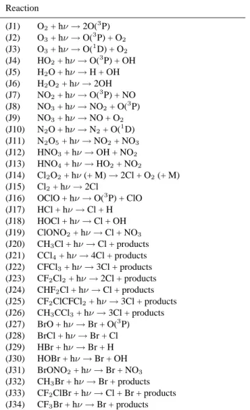
Table 2. Photolysis reactions included in the model
Reaction (J1) O2+ hν → 2O(3P) (J2) O3+ hν → O(3P) + O2 (J3) O3+ hν → O(1D) + O2 (J4) HO2+ hν → O(3P) + OH (J5) H2O + hν → H + OH (J6) H2O2+ hν → 2OH (J7) NO2+ hν → O(3P) + NO (J8) NO3+ hν → NO2+ O(3P) (J9) NO3+ hν → NO + O2 (J10) N2O + hν → N2+ O(1D) (J11) N2O5+ hν → NO2+ NO3 (J12) HNO3+ hν → OH + NO2 (J13) HNO4+ hν → HO2+ NO2 (J14) Cl2O2+ hν (+ M) → 2Cl + O2(+ M) (J15) Cl2+ hν → 2Cl (J16) OClO + hν → O(3P) + ClO (J17) HCl + hν → Cl + H (J18) HOCl + hν → Cl + OH (J19) ClONO2+ hν → Cl + NO3 (J20) CH3Cl + hν → Cl + products (J21) CCl4+ hν → 4Cl + products (J22) CFCl3+ hν → 3Cl + products (J23) CF2Cl2+ hν → 2Cl + products (J24) CHF2Cl + hν → Cl + products (J25) CF2ClCFCl2+ hν → 3Cl + products (J26) CH3CCl3+ hν → 3Cl + products (J27) BrO + hν → Br + O(3P) (J28) BrCl + hν → Br + Cl (J29) HBr + hν → Br + H (J30) HOBr + hν → Br + OH (J31) BrONO2+ hν → Br + NO3 (J32) CH3Br + hν → Br + products (J33) CF2ClBr + hν → Cl + Br + products (J34) CF3Br + hν → Br + products
The term “products” represents constituents which are not consid-ered in the present study.
of hydrogen, chlorine and bromine radicals. These source gases (marked by superscript a in Table 1) are assumed to be unaffected by transport and chemistry. Constant latitude-height distributions are taken into account for these com-pounds (see below). In order to minimize the numerical stiffness of the differential equations describing the chemical system, several highly reactive species, with chemical life times much smaller than transport timescales, are grouped into the families Ox:=O(1D)+O(3P)+O3, NOx:=NO+NO2,
HOx:=H+OH +HO2, ClOx:=Cl+ClO and BrOx:=Br+BrO.
The continuity equations for the transported species are solved using the operator splitting technique. A semi-implicit method is employed to calculate the chemical con-tributions to concentration changes:
ni(t + ∆t) = (ni(t) + Pi∆t)/(1 + [Li/ni(t)]∆t), (1)
where ni is the concentration of species i, Pi and Li are
respec-T -2KNAT TIce T TSAT T -3KIce STS / NAT - scheme H2SO4 / H2O NAT + SAT
Ice + NAT + SAT
H2SO4 / HNO3 / H2O SAT
H2SO4 / H2O
Figure 1
Fig. 1. Schematic overview of the particle types and the phase
tran-sition pathways considered in the standard version of the model (STS/NAT-scheme, see Sect. 2.3.1 for details).
tively, and ∆t is the chemical time step which is chosen as
∆t = 225 s in the current model version. Since Eq. (1)
is not necessarily mass conserving, a scaling procedure is applied which adjusts the total mass of nitrogen, chlorine and bromine atoms contained in a respective grid box to the values encountered before chemical integration. Assuming steady-state, the concentrations of the short-lived nontrans-ported constituents at time t + ∆t are determined from the concentrations evaluated by Eq. (1).
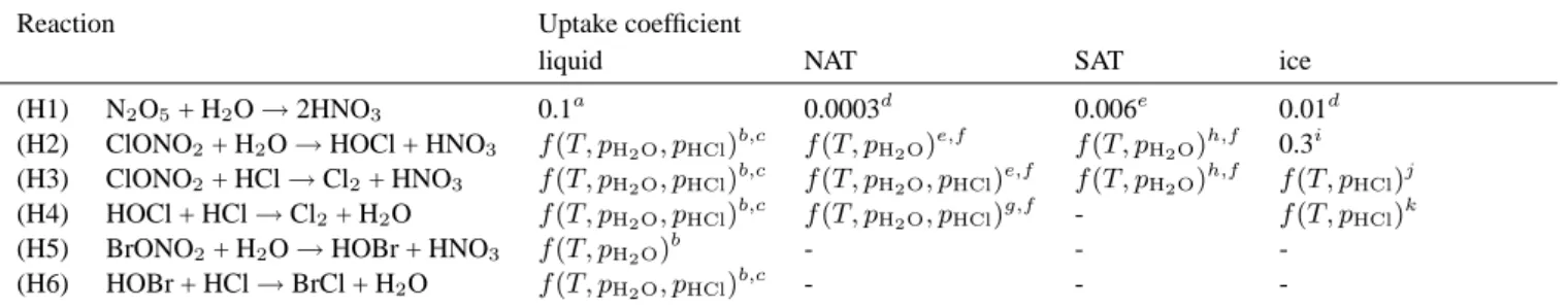
The chemical mechanism includes 34 photolytic reac-tions, 114 gas-phase collision reactions and 6 heteroge-neous reactions on liquid binary H2SO4/H2O and ternary
H2SO4/HNO3/H2O solution aerosols, as well as NAT,
sul-furic acid tetrahydrate (SAT) and ice particles. The set of reactions and the rate coefficients considered are listed in Ta-bles 2, 3 and 4.
The rate coefficients of the photodissociation reactions are evaluated from a precalculated look-up table (G. Brasseur, personal communication, 1993) which includes the needed photolysis rates dependent on solar zenith angle, altitude, ozone column above the considered location and surface albedo. The methodology for derivation of the photoly-sis constants was described, for instance, by Brasseur et al. (1990) or Granier and Brasseur (1992). Several updates have been made to the absorption cross sections of the con-sidered species, including the temperature dependence of the HNO3(Rattigan et al., 1992) and the ClONO2(Burkholder et
al., 1994) cross sections. The photodissociation of bromine compounds was added to the model considering absorption cross sections, as recommended by DeMore et al. (1997). The adsorption cross sections of HOBr and HBr were cho-sen according to Orlando and Burkholder (1995) and Good-eve and Taylor (1935), respectively. The rate coefficients of the gas phase collision reactions are chosen according to
De-More et al. (1997) with the exceptions of reactions (R48), (R54), (R56) and (R72) which are treated following the rec-ommendations of Baulch et al. (1981). The rates of the het-erogeneous reactions are determined in analogy to the work of Hendricks et al. (1999) taking into account possible dif-fusion limitation of gas-to-particle mass fluxes. The uptake coefficients are evaluated as described in Table 4. The cal-culation of the surface area concentrations and characteristic sizes of the respective aerosol and PSC particles is described in Sect. 2.3.
The initial concentrations of the non-bromine containing chemical trace constituents were chosen according to the re-sults of 2-D simulations performed by Brasseur et al. (1990). The concentrations of bromine compounds were initialized using the vertical profiles of bromine constituent concentra-tions calculated with a 1-D model by Kr¨uger and Fabian (1986). The total abundances of inorganic chlorine and bromine compounds were adjusted to “present-day” con-ditions as simulated with the global AER 2-D model (D. K. Weisenstein, personal communication, 1997), resulting in total upper stratospheric concentrations of 3.2 ppbv and 19.0 pptv, respectively. For a description of the AER model see, for instance, Weisenstein et al. (1996). In order to sim-ulate stratospheric ozone distributions encountered during real episodes, model ozone was initialized using UARS-MLS data (see above).
2.3 The microphysical module
The COMMA microphysical module enables the evaluation of microphysical parameters relevant for the simulation of reactive and nonreactive uptake of trace constituents on and in stratospheric aerosol and PSC particles. Volume concen-trations, surface area concentrations and characteristic sizes of liquid binary H2SO4/H2O and ternary H2SO4/HNO3/H2O
solution aerosols as well as NAT, SAT and ice particles are evaluated. A schematic overview of the particle types and phase transition pathways considered in the standard version of the module (STS/NAT-scheme, Sect. 2.3.1) is displayed in Fig. 1. In addition to the standard microphysical scheme, two alternative PSC formation schemes are employed for the present study (Sect. 2.3.2).
2.3.1 The STS/NAT-scheme
The composition and volume concentration of liquid parti-cles are calculated from modelled H2SO4, HNO3, H2O and
temperature employing the method developed by Carslaw et al. (1995). The liquid aerosol surface area concentration as well as the liquid particle sizes which are key parame-ters controlling the rates of heterogeneous processes are in-ferred from the volume concentration assuming a unimodal lognormal size distribution. A total particle number concen-tration of N = 10 cm−3 and a geometric standard devia-tion of σ = 2 are considered as size distribudevia-tion parameters typical for the lower stratospheric background aerosol (Hof-mann, 1990; Deshler et al., 1993). The initial spatial
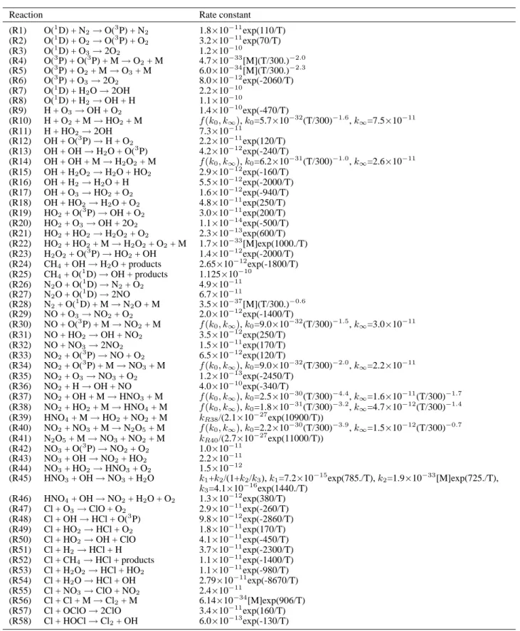
distri-Table 3. Gas phase reactions included in the model. Rate constants for first- and second-order reactions are given in units of s−1 and molecules−1cm3s−1, respectively. Rate constants for third-order reactions are given as effective second-order rate constants in units of molecules−1cm3s−1
Reaction Rate constant
(R1) O(1D) + N2→ O(3P) + N2 1.8×10⁻¹¹exp(110/T) (R2) O(1D) + O2→ O(3P) + O2 3.2×10⁻¹¹exp(70/T) (R3) O(1D) + O3→ 2O2 1.2×10⁻¹⁰ (R4) O(3P) + O(3P) + M → O 2+ M 4.7×10⁻³³[M](T/300.)−2.0 (R5) O(3P) + O 2+ M → O3+ M 6.0×10⁻³⁴[M](T/300.)−2.3 (R6) O(3P) + O3→ 2O2 8.0×10⁻¹²exp(-2060/T) (R7) O(1D) + H2O → 2OH 2.2×10⁻¹⁰ (R8) O(1D) + H2→ OH + H 1.1×10⁻¹⁰ (R9) H + O3→ OH + O2 1.4×10⁻¹⁰exp(-470/T) (R10) H + O2+ M → HO2+ M f (k0, k∞), k0=5.7×10⁻³²(T/300)−1.6, k∞=7.5×10⁻¹¹ (R11) H + HO2→ 2OH 7.3×10⁻¹¹ (R12) OH + O(3P) → H + O2 2.2×10⁻¹¹exp(120/T) (R13) OH + OH → H2O + O(3P) 4.2×10⁻¹²exp(-240/T) (R14) OH + OH + M → H2O2+ M f (k0, k∞), k0=6.2×10⁻³¹(T/300)−1.0, k∞=2.6×10⁻¹¹ (R15) OH + H2O2→ H2O + HO2 2.9×10⁻¹²exp(-160/T) (R16) OH + H2→ H2O + H 5.5×10⁻¹²exp(-2000/T) (R17) OH + O3→ HO2+ O2 1.6×10⁻¹²exp(-940/T) (R18) OH + HO2→ H2O + O2 4.8×10⁻¹¹exp(250/T) (R19) HO2+ O(3P) → OH + O2 3.0×10⁻¹¹exp(200/T) (R20) HO2+ O3→ OH + 2O2 1.1×10⁻¹⁴exp(-500/T) (R21) HO2+ HO2→ H2O2+ O2 2.3×10⁻¹³exp(600/T) (R22) HO2+ HO2+ M → H2O2+ O2+ M 1.7×10⁻³³[M]exp(1000./T) (R23) H2O2+ O(3P) → HO2+ OH 1.4×10⁻¹²exp(-2000/T) (R24) CH4+ OH → H2O + products 2.65×10⁻¹²exp(-1800/T) (R25) CH4+ O(1D) → OH + products 1.125×10⁻¹⁰ (R26) N2O + O(1D) → N2+ O2 4.9×10⁻¹¹ (R27) N2O + O(1D) → 2NO 6.7×10⁻¹¹ (R28) N2+ O(1D) + M → N2O + M 3.5×10−37[M](T/300.)−0.6 (R29) NO + O3→ NO2+ O2 2.0×10⁻¹²exp(-1400/T) (R30) NO + O(3P) + M → NO2+ M f (k0, k∞), k0=9.0×10⁻³²(T/300)−1.5, k∞=3.0×10⁻¹¹ (R31) NO + HO2→ OH + NO2 3.5×10⁻¹²exp(250/T) (R32) NO + NO3→ 2NO2 1.5×10⁻¹¹exp(170/T) (R33) NO2+ O(3P) → NO + O2 6.5×10⁻¹²exp(120/T) (R34) NO2+ O(3P) + M → NO3+ M f (k0, k∞), k0=9.0×10⁻³²(T/300)−2.0, k∞=2.2×10⁻¹¹ (R35) NO2+ O3→ NO3+ O2 1.2×10⁻¹³exp(-2450/T) (R36) NO2+ H → OH + NO 4.0×10⁻¹⁰exp(-340/T) (R37) NO2+ OH + M → HNO3+ M f (k0, k∞), k0=2.5×10⁻³⁰(T/300)−4.4, k∞=1.6×10⁻¹¹(T/300)−1.7 (R38) NO2+ HO2+ M → HNO4+ M f (k0, k∞), k0=1.8×10⁻³¹(T/300)−3.2, k∞=4.7×10⁻¹²(T/300)−1.4 (R39) HNO4+ M → HO2+ NO2+ M kR38/(2.1×10−27exp(10900/T)) (R40) NO2+ NO3+ M → N2O5+ M f (k0, k∞), k0=2.2×10⁻³⁰(T/300)−3.9, k∞=1.5×10⁻¹²(T/300)−0.7 (R41) N2O5+ M → NO3+ NO2+ M kR40/(2.7×10−27exp(11000/T)) (R42) NO3+ O(3P) → NO2+ O2 1.0×10⁻¹¹ (R43) NO3+ OH → NO2+ HO2 2.2×10⁻¹¹ (R44) NO3+ HO2→ HNO3+ O2 1.5×10⁻¹²
(R45) HNO3+ OH → NO3+ H2O k1+k2/(1+k2/k3), k1=7.2×10⁻¹⁵exp(785./T), k2=1.9×10⁻³³[M]exp(725./T),
k3=4.1×10⁻¹⁶exp(1440./T) (R46) HNO4+ OH → NO2+ H2O + O2 1.3×10⁻¹²exp(380/T) (R47) Cl + O3→ ClO + O2 2.9×10⁻¹¹exp(-260/T) (R48) Cl + OH → HCl + O(3P) 9.8×10⁻¹²exp(-2860/T) (R49) Cl + HO2→ HCl + O2 1.8×10⁻¹¹exp(170/T) (R50) Cl + HO2→ OH + ClO 4.1×10⁻¹¹exp(-450/T) (R51) Cl + H2→ HCl + H 3.7×10⁻¹¹exp(-2300/T) (R52) Cl + CH4→ HCl + products 1.1×10⁻¹¹exp(-1400/T) (R53) Cl + H2O2→ HCl + HO2 1.1×10⁻¹¹exp(-980/T) (R54) Cl + H2O → HCl + OH 2.79×10⁻¹¹exp(-8670/T) (R55) Cl + NO3→ ClO + NO2 2.4×10⁻¹¹ (R56) Cl + Cl + M → Cl2+ M 6.14×10⁻³⁴[M]exp(906/T)
(R57) Cl + OClO → 2ClO 3.4×10⁻¹¹exp(160/T)
Table 3. (continued)
Reaction Rate constant
(R59) Cl + Cl2O2→ Cl + Cl2+ O2 1.0×10⁻¹⁰
(R60) Cl + ClONO2→ Cl2+ NO3 6.5×10⁻¹²exp(135/T)
(R61) ClO + O(3P) → Cl + O2 3.0×10⁻¹¹exp(70/T)
(R62) ClO + OH → Cl + HO2 1.1×10⁻¹¹exp(120/T)
(R63) ClO + HO2→ HOCl + O2 4.8×10⁻¹³exp(700/T)
(R64) ClO + NO → Cl + NO2 6.4×10⁻¹²exp(290/T)
(R65) ClO + NO2+ M → ClONO2+ M f (k0, k∞), k0=1.8×10⁻³¹(T/300)−3.4, k∞=1.5×10⁻¹¹(T/300)−1.9
(R66) ClO + NO3→ Cl + NO2+ O2 4.7×10⁻¹³
(R67) ClO + ClO + M → Cl2O2+ M f (k0, k∞), k0=2.2×10⁻³²(T/300)−3.1, k∞=3.5×10⁻¹²(T/300)−1.0
(R68) Cl2O2+ M → 2ClO + M kR67/(1.3×10−27exp(8744/T))
(R69) OClO + O(3P) → ClO + O2 2.4×10⁻¹²exp(-960/T)
(R70) OClO + OH → HOCl + O2 4.5×10⁻¹³exp(800/T)
(R71) OClO + NO → ClO + NO2 2.5×10⁻¹²exp(-600/T)
(R72) Cl2+ M → 2Cl + M exp(ln(3.85×10⁻¹¹[M]) - 23630/T) (R73) Cl2+ O(1D) → ClO + Cl 2.8×10⁻¹⁰(25% quenching) (R74) Cl2+ OH → HOCl + Cl 1.4×10⁻¹²exp(-900/T) (R75) HCl + O(1D) → OH + Cl 1.0×10⁻¹⁰ (R76) HCl + O(1D) → H + ClO 3.6×10⁻¹¹ (R77) HCl + O(3P) → Cl + OH 1.0×10⁻¹¹exp(-3300/T) (R78) HCl + OH → Cl + H2O 2.6×10⁻¹²exp(-350/T)
(R79) HOCl + O(3P) → ClO + OH 1.0×10⁻¹¹exp(-1300/T)
(R80) HOCl + OH → ClO + H2O 3.0×10⁻¹²exp(-500/T)
(R81) ClONO2+ O(3P) → ClO + NO3 2.9×10⁻¹²exp(-800/T)
(R82) ClONO2+ OH → HOCl + NO3 1.2×10⁻¹²exp(-330/T)
(R83) CH3Cl + O(1D) → ClO + products 4.0×10⁻¹⁰
(R84) CH3Cl + OH → H2O + products 4.0×10⁻¹²exp(-1400/T)
(R85) CCl4+ O(1D) → ClO + products 3.3×10⁻¹⁰(14% quenching)
(R86) CFCl3+ O(1D) → ClO + products 2.3×10⁻¹⁰(40% quenching)
(R87) CF2Cl2+ O(1D) → ClO + products 1.4×10⁻¹⁰(14% quenching)
(R88) CHF2Cl + O(1D) → ClO + products 1.0×10⁻¹⁰(28% quenching)
(R89) CHF2Cl + OH → H2O + products 1.0×10⁻¹²exp(-1600/T) (R90) CF2ClCFCl2+ O(1D) → ClO + products 2.0×10⁻¹⁰ (R91) CH3CCl3+ O(1D) → ClO + products 4.0×10⁻¹⁰ (R92) CH3CCl3+ OH → H2O + products 1.8×10⁻¹²exp(-1550/T) (R93) Br + O3→ BrO + O2 1.7×10⁻¹¹exp(-800/T) (R94) Br + HO2→ HBr + O2 1.5×10⁻¹¹exp(-600/T)
(R95) Br + OClO → BrO + ClO 2.6×10⁻¹¹exp(-1300/T)
(R96) BrO + O(3P) → Br + O
2 1.9×10⁻¹¹exp(230/T)
(R97) BrO + OH → Br + HO2 7.5×10⁻¹¹
(R98) BrO + HO2→ HOBr + O2 3.4×10⁻¹²exp(540/T)
(R99) BrO + NO → Br + NO2 8.8×10⁻¹²exp(260/T)
(R100) BrO + NO2+ M → BrONO2+ M f (k0, k∞), k0=5.2×10⁻³¹(T/300)−3.2, k∞=6.9×10⁻¹²(T/300)−2.9
(R101) BrO + ClO → Br + OClO 1.6×10⁻¹²exp(430/T)
(R102) BrO + ClO (+ M) → Br + Cl + O2(+ M) 2.9×10⁻¹²exp(220/T)
(R103) BrO + ClO → BrCl + O2 5.8×10⁻¹³exp(170/T)
(R104) BrO + BrO → 2Br + O2 1.5×10⁻¹²exp(230/T)
(R105) HBr + O(1D) → OH + Br 1.5×10⁻¹⁰(20% quenching)
(R106) HBr + O(3P) → Br + OH 5.8×10⁻¹²exp(-1500/T)
(R107) HBr + OH → Br + H2O 1.1×10⁻¹¹
(R108) HOBr + O(3P) → OH + BrO 1.2×10⁻¹⁰exp(-430/T)
(R109) HOBr + OH → H2O + BrO 1.1×10⁻¹²
(R110) HOBr + Cl → HCl + BrO 1.1×10⁻¹⁰
(R111) CH3Br + O(1D) → BrO + products 1.8×10⁻¹⁰
(R112) CH3Br + OH → H2O + products 4.0×10⁻¹²exp(-1470/T)
(R113) CF2ClBr + O(1D) → BrO + products 1.5×10⁻¹⁰(36% quenching)
(R114) CF3Br + O(1D) → BrO + products 1.0×10⁻¹⁰(59% quenching)
M ∈ {N2, O2}. For third-order reactions, f (k0, k∞) has to be evaluated according to DeMore et al. (1997): f (k0, k∞) = (k0[M]/(1 + k0[M]/k∞)) × 0.6(1+(log10(k0[M]/k∞))
2)−1
. The term “products” represents constituents which are not considered in the present study.
Table 4. Heterogeneous reactions included in the model
Reaction Uptake coefficient
liquid NAT SAT ice
(H1) N2O5+ H2O → 2HNO3 0.1a 0.0003d 0.006e 0.01d
(H2) ClONO2+ H2O → HOCl + HNO3 f (T, pH2O, pHCl)
b,c f (T, pH2O) e,f f (T, pH2O) h,f 0.3i (H3) ClONO2+ HCl → Cl2+ HNO3 f (T, pH2O, pHCl) b,c f (T, p H2O, pHCl) e,f f (T, p H2O) h,f f (T, p HCl)j (H4) HOCl + HCl → Cl2+ H2O f (T, pH2O, pHCl) b,c f (T, p H2O, pHCl) g,f - f (T, pHCl)k
(H5) BrONO2+ H2O → HOBr + HNO3 f (T, pH2O)
b - -
-(H6) HOBr + HCl → BrCl + H2O f (T, pH2O, pHCl)b,c - -
-a
DeMore et al. (1997);bas described by Hendricks et al. (1999);cHHClfor ternary solutions from Luo et al. (1995);dHanson and
Ravis-hankara (1993a);eHanson and Ravishankara (1993b);fCarslaw et al. (1997) (“scheme 1”);gAbbatt and Molina (1992);hZhang et al. (1994);
i
Hanson and Ravishankara (1991); jas described by Drdla et al. (1993), data from Leu (1988) and Hanson and Mauersberger (1990);
kγ = 0.3 × γ(H3)/γ
max(H3) (γ as recommended by De More et al. (1997), but with (T , pHCl)-dependence as γ(H3))
bution of sulfate mass is derived applying the inverse of the procedure described above to aerosol surface area concentra-tions as recommended by the WMO (1992) for stratospheric background aerosol conditions which can be assumed for the considered winter (Thomason et al., 1997).
It is assumed that formation of solid particles is initiated by the freezing of supercooled ternary solution particles at temperatures of 3 K below the ice frost point Tice (Koop
et al., 1995) in order to form ice crystals. The ice volume concentration is calculated assuming thermodynamic equi-librium. Taking into account an ice particle number concen-tration of 0.01 cm−3(e.g. Dye et al., 1992), the ice particle surface area concentration is evaluated with the simplifying assumption of ice particles showing spherical geometry and a monodisperse size distribution. Since NAT can nucleate heterogeneously on ice surfaces (Koop et al., 1997a, 1997b), it is assumed that NAT is incorporated into the ice particles during the freezing process. The NAT volume concentration is inferred from thermodynamic equilibrium constraints us-ing the vapor pressure data provided by Hanson and Mauers-berger (1988).
Mechanisms of SAT formation in the stratosphere are presently not fully understood. It is suggested that SAT forms by the heterogeneous freezing of sulfuric acid on ice particles rather than by homogeneous freezing processes (Koop et al., 1997a, 1997b). However, there is presently little evidence for SAT in the stratosphere (Carslaw et al., 1999). Hence, we assume that only a portion of the liquid particles are in-volved in the freezing processes. In the model simulations, 1 liquid particle per cubic centimeter is consumed by the freez-ing process described above and is incorporated as SAT into ice crystals. The coexistence of the remaining liquid sulfate aerosols and the solid particles fulfills thermodynamic sta-bility requirements (Koop et al., 1997a). The number con-centration of liquid particles involved in the freezing pro-cesses was chosen in correspondence to the respective SAT or NAT particle number concentration: a value of 1 cm−3 is generally considered as the particle number concentration of stratospheric crystalline hydrates (NAT or SAT). This is primarily motivated by the in situ measurements by Dye et
al. (1992) performed in the Arctic lower stratosphere. Dye et al. (1992) found NAT particle number concentrations of 2–16 cm−3. They further discussed that these number con-centrations are a factor of 2–3 higher than the condensation nuclei concentrations detected outside the PSCs. Since they could not explain this discrepancy, we decided to use the NAT and for consistency sake also the SAT number concen-tration of 1 cm−3 which shows a better correspondence to the condensation nuclei concentrations observed.
Ice particles are assumed to evaporate above Tice
leav-ing NAT. The NAT surface area concentration is evaluated in analogy to that of ice particles, taking into account spher-ical geometry and a monodisperse size distribution. NAT is thermodynamically stable as long as the temperatures stay below the NAT equilibrium temperature TNAT (Hanson and
Mauersberger, 1988). If the temperature again falls below
Tice, we assume that ice nucleates heterogeneously on the
NAT surfaces (Koop et al., 1997a). If the temperature ex-ceeds TNAT, NAT is assumed to evaporate and leave behind
SAT. After preactivation of the SAT surface by an initial de-position of NAT, heterogeneous nucleation of NAT on SAT can occur at supersaturations SNATaround 10
(correspond-ing to temperatures of 2–3 K below TNAT) (Zhang et al.,
1996). In our simulations, SAT can act as an agent for NAT formation in the case of SNAT ≥ 10. We further assume
that SAT particles are transformed to liquid sulfate aerosols at temperatures above the SAT melting point TSAT(Zhang et
al., 1993).
2.3.2 Alternative PSC schemes
Two alternative PSC schemes can optionally be applied. First, a PSC scheme promoting solid particle formation is available. We will refer to this approach as the “NAT-scheme”, where it is assumed that NAT can form whenever NAT equilibrium can be established (T < TNAT). Hence,
NAT can form at any NAT supersaturation, regardless of whether SAT is present. Thus, the NAT-scheme represents an upper limit for NAT particle occurrence. Similar to the STS/NAT-scheme, it is assumed in the NAT-scheme that a number of sulfate aerosols of 1 cm−3 is consumed by solid
Figure 2
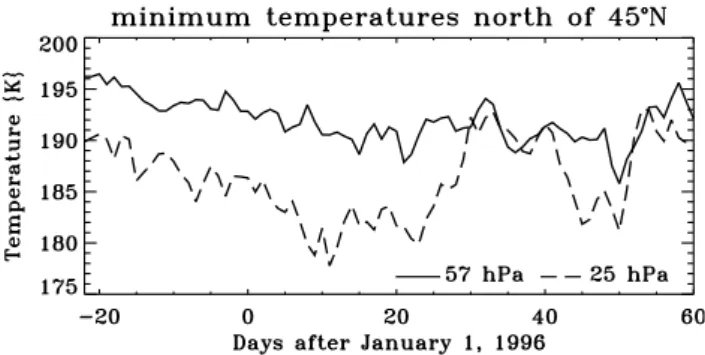
Fig. 2. Temporal change of model minimum temperatures within
the area north of 45◦N. Data is presented for the time period be-tween 10 December 1995, and 29 February 1996, and the model levels 57 and 25 hPa.
particle formation and that the rest of the sulfate aerosols re-main liquid. As in the STS/NAT-scheme, ice nucleates on NAT particles if the temperature falls below Tice and NAT
particles leave behind SAT after evaporation. Particle num-ber concentrations of 10 cm−3, 1 cm−3 and 0.01 cm−3 are assumed for liquid sulfate aerosols, NAT (or SAT) and ice particles, respectively. Second, a PSC scheme which we will refer to as the “STS-scheme” can be employed, where freez-ing processes are not considered. Hence, particles are gen-erally in the liquid phase. PSC particles are formed by the uptake of HNO3and water into liquid sulfuric acid aerosols.
A number concentration of 10 cm−3is assumed. The micro-physical parameters relevant for chemical processing used when the NAT- or the STS-scheme is in consideration are evaluated in analogy to the STS/NAT-scheme (Sect. 2.3.1). For a summary of the PSC-schemes applied, see Table 5.
3 Simulations
As in a previous study by G¨unther and Baier (1998), the COMMA model was employed to simulate stratospheric dy-namics and chemistry of the Arctic polar vortex during the winter 1995/96, which was characterized by comparatively low temperatures and an effective ozone loss (Manney et al., 1996a). In the present study, we focus in particular on the coldest period of that winter, which extended from mid-December 1995 to the end of February 1996. During this time, most of the PSC activity occurred. The model exper-iments were performed for the period between 10 Decem-ber 1995, and 29 February 1996. The simulations were ini-tialized using MLS ozone data as well as the results of a spin-up simulation covering the period between 25 Novem-ber 1995, and 9 DecemNovem-ber 1995. The model spin-up pro-vides chemical consistency and adjusts the chemical con-stituent spatial distributions to the dynamical conditions en-countered at the start date of the main simulations. The ini-tial trace gas concentrations in the spin-up model run were chosen as described in Sect. 2.2. In order to investigate the potential of different PSC types for chlorine activation and the corresponding ozone depletion, different model runs
Figure 3
Fig. 3. Temporal change of particle surface area concentrations
(µm2 cm−3) averaged over the area north of 45◦N on the model
levels (bottom frame) 57 hPa and (top frame) 25 hPa. Data is presented for the time period between 10 December 1995, and 29 February 1996, simulated in the model experiments performed with the NAT- and the STS-scheme, respectively.
were performed. First, the standard microphysical scheme (Sect. 2.3.1) called the STS/NAT-scheme was applied. Sec-ond, sensitivity studies were performed considering the STS-scheme and the NAT-STS-scheme described in Sect. 2.3.2. An additional model experiment where PSC formation is ne-glected and consequently, where heterogeneous chemistry is restricted to reactions on liquid binary sulfate aerosols is used as a reference simulation for evaluating the PSC impact on atmospheric chemistry. The corresponding microphysical scheme is referred to as the “BIN-scheme” (Table 5).
The temporal development of the model minimum tem-peratures occurring north of 45◦N on the two coldest model levels, 57 hPa (approximately 19 km altitude) and 25 hPa (approximately 25 km altitude), is shown in Fig. 2. Since the model is driven by ECMWF analysis below 10 hPa (Sect. 2.1), the data represents ECMWF temperatures inter-polated on the model grid. The minimum temperature stays below 195 K during almost the entire simulated period at both model levels. Since 195 K approximately corresponds to the NAT formation threshold temperature, NAT particles potentially could occur during prolonged time periods. Ice particle formation was promoted on the 25 hPa level due to very low temperatures, especially during January and
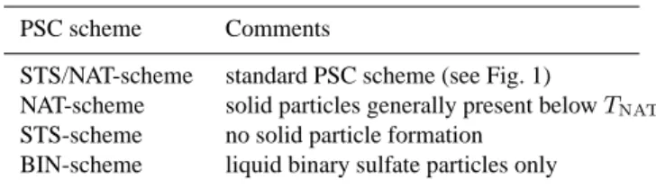
mid-Table 5. PSC schemes applied (see text for details)
PSC scheme Comments
STS/NAT-scheme standard PSC scheme (see Fig. 1)
NAT-scheme solid particles generally present below TNAT
STS-scheme no solid particle formation
BIN-scheme liquid binary sulfate particles only
February 1996.
The temporal development of surface area concentrations of different particle types modelled employing the NAT- and the STS-scheme is presented in Fig. 3 for the 57 hPa and the 25 hPa level. The data was averaged over the domain north of 45◦N. A circumpolar averaging domain was chosen, rather than only the vortex area, in order to avoid a depen-dence of the results on the vortex area definition and to ad-equately include PSCs located at the vortex edge (occurring especially during the late winter). The threshold of 45◦N was chosen since PSC activity as well as the related chlorine activation (see below) were almost totally restricted to ar-eas north of that latitude. The simulation performed with the NAT-scheme demonstrates that the potential for NAT particle existence (NAT equilibrium conditions) was present at both pressure levels, especially during January and mid-February when the lowest temperatures occurred. Ice particles are formed in the NAT-scheme case preferently at 25 hPa during January. The relatively large mean surface area concentra-tion of liquid particles in the NAT-scheme simulaconcentra-tion results from sulfate aerosols being omnipresent with significant con-centrations throughout the area considered. The simulation with the STS-scheme which includes only liquid particles is represented by the dotted line. Large deviations from the modelled liquid aerosol surface area concentration obtained with NAT-scheme occur during mid-February at 57 hPa, and during January and mid-February at 25 hPa. This is a conse-quence of the effective uptake of HNO3and water into
liq-uid particles simulated in the STS-scheme model run for the coldest periods of the winter. The results presented in Fig. 3 reveal that occurrences of large liquid surface areas in the STS-case mostly are of a shorter duration when compared to the PSC events simulated in the NAT-case. Horizontal distri-butions of PSC surface area concentrations at 57 and 25 hPa, as simulated considering the NAT- and the STS-scheme are shown in Fig. 4. The results are presented for days of com-paratively large surface area concentrations in both simula-tions. Since chlorine activation was most effective in Jan-uary (see below), we focus in particular on that month. The characteristic difference between the two PSC types is that large surface area concentrations of liquid PSC particles in the simulation with the STS-scheme are restricted to smaller spatial areas compared to the areas covered by PSCs formed by solid particles in the NAT-scheme simulation. Similar to the work of Carslaw et al. (1997), it can be concluded that areas where NAT particles can potentially exist in equilib-rium (T < TNAT) appear to be significantly larger and occur
over longer time periods compared to the areas showing con-ditions appropriate for large liquid particle formation.
In the simulations performed with the STS/NAT-scheme (not figured), solid particle occurrences are primarily re-stricted to the January 25 hPa level, where model temper-atures occasionally fall below the threshold of Tice− 3 K.
This induces freezing of ternary solution droplets resulting in effective solid particle formation. As a consequence, PSCs encountered during January at 25 hPa in the STS/NAT simulation are primarily composed of NAT or ice particles. The strong temperature increase occurring in late January at 25 hPa leads to evaporation of these PSCs and subsequently to melting of SAT. Since model stratospheric temperatures stay primarily above Tice− 3 K during February, solid PSC
particle formation occurs only very sparsely during February in the STS/NAT case.
As a consequence of the PSC activity discussed above, an effective production of active chlorine is simulated. Chlorine activation was also observed during the winter 1995/96 by means of ClO measurements taken with the UARS-MLS in-strument (Santee et al., 1996; Waters et al., 1996). In order to validate the model ClO, a comparison with the MLS data was performed. Due to the large noise inherent in the MLS ClO, a comparison of local ClO concentrations is difficult. Hence, similar to the work of Massie et al. (2000), we eval-uated the temporal evolution of spatially averaged ClO data. Figure 5 shows the temporal development of MLS (version 4) and the model ClO averaged over the model levels located at 57 and 25 hPa. MLS ClO is plotted for the time peri-ods available in the MLS data set (see below). Model re-sults are presented for the simulations including PSC effects (the NAT-, the STS, and the STS/NAT-scheme simulation). For the same reasons as in the case of the particle surface area concentrations (Fig. 3), averages were calculated over the area northward of 45◦N. Data northward of 80◦N was not included since this area was not covered by the MLS ob-servations. In order to exclude inconsistencies caused by the diurnal variation of the ClO concentration, we only take into account daytime ClO which has the additional advantage that it can be taken as an approximation to the full extent of active chlorine. The MLS ClO data points considered were selected as recommended by Waters et al. (1996). Only those days of sufficient availability of daytime data points were taken into account. The error bars were calculated on the basis of the accuracies and the single profile precisions recommended by L. Froidevaux et al. (http://mls.jpl.nasa.gov; see also Massie et al., 2000).
The comparison reveals that the model results resemble the MLS data most of the time within the measurement er-ror range. Strong deviations between the model and the observations occur especially during the end of January at 25 hPa when averaged model ClO exceeds the upper limit of the MLS tolerance. Significant deviations also occur during February when the model tends to show larger ClO amounts at 25 hPa and lower values at 57 hPa. However, these discrep-ancies primarily stay within the MLS error. Generally, the large noise of MLS ClO hampers a more quantitative
evalu-NAT-scheme
STS-scheme
solid particles
liquid particles
25 hPa, 12 January 1996
57 hPa, 22 January 1996
surface area concentration [
µ
m cm ]
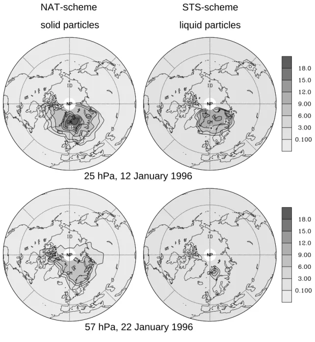
2 −3Fig. 4. Surface area concentration (µm2 cm−3) of different particle types modelled for (top frames) the 25 hPa and (bottom frames) the 57 hPa levels. Results are shown for two selected days of January 1996 showing comparatively large PSC activity (57 hPa level on 22 January 1996, and 25 hPa level on 12 January 1996). The left frames show the total solid particle surface area concentration (NAT, SAT and ice particles) modelled applying the NAT-scheme. The right frames present the surface area concentration of liquid particles simulated using the STS-scheme.
ation of the model quality. The comparison also suffers from large measurement gaps in the MLS data during the time pe-riod considered. The variation of model ClO caused by the assumption of different PSC microphysical schemes is small compared to the MLS error. Hence, the comparison of model ClO to MLS data can only be helpful in terms of a rough model validation, rather than in identifying the most realistic PSC microphysical code. It can be concluded that the model
is able to reproduce observed chlorine activation in a qualita-tively reasonable manner. Most of the time during MLS data availability, deviations between modelled and observed ClO stay within the MLS error range.
Compared to the model study by Massie et al. (2000) which focusses on chlorine activation during December 1995 and early January 1996, the COMMA simulations appear to show a less effective mid-December chlorine activation at
0 0.1 0.2 0.3 0.4 -20 -10 0 10 20 30 40 50 60 0 0.1 0.2 0.3 0.4 -20 -10 0 10 20 30 40 50 60
Days after January 1, 1996 mean ClO north of 45°N
Mean ClO {ppbv} 25 hPa 57 hPa 0.40 0.30 0.20 0.10 0.00 NAT-scheme STS/NAT-scheme STS-scheme MLS Mean ClO {ppbv} 0.40 0.30 0.20 0.10 0.00 -20 0 20 40 60 -20 0 20 40 60 Figure 5
Fig. 5. Temporal change of the ClO mixing ratio (ppbv) averaged
over the area between 45◦N and 80◦N. Model results are shown as obtained with the COMMA model applying the NAT-, the STS- and the STS/NAT-scheme, respectively. For comparison, correspond-ing average ClO concentrations derived from UARS-MLS observa-tional data as well as the potential MLS ClO errors are presented. Data is shown for the model levels (bottom frame) 57 hPa and (top frame) 25 hPa and the time period between 10 December 1995, and 29 February 1996. Only daytime ClO data is taken into account. See text for details.
lower stratospheric pressure levels. Compared to the MLS data, chlorine activation during mid-December is less effec-tive at 57 hPa in the COMMA simulations. In the results of Massie et al. obtained for 46 and 100 hPa, mean daytime ClO concentrations during mid-December are larger than corre-sponding MLS values. Since temperatures were very close to the type 1 PSC formation thresholds during this time pe-riod, the discrepancies between the two models may result from differences in the PSC microphysical representation and also from temperature differences between the U.K. Me-teorological Office (UKMO) data used in the work of Massie et al. (2000) and the ECMWF data set employed here. Knud-sen et al. (1996) compared ECMWF analysis data to balloon bourne measurements taken during the winter 1994/95 in the arctic vortex at pressure levels around 50 hPa. They found that ECMWF temperatures were on average 2.4 K higher compared to the in situ measurements. In a similar study by Manney et al. (1996b), average warm biases of UKMO-analyses of 0.5–1.9 K were calculated for different periods of the same winter. Hence, ECMWF temperatures appear to show a larger average warm bias compared to UKMO
analy-Figure 6
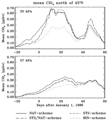
Fig. 6. Temporal change of the ClOx(:=Cl + ClO +
2 Cl2O2+2 Cl2+HOCl+OClO) mixing ratio (ppbv) averaged over
the area north of 45◦N on the model levels (bottom frame) 57 hPa
and (top frame) 25 hPa. Results are presented for the time pe-riod between 10 December 1995, and 29 February 1996, simulated in the model experiments performed with the NAT-, the STS-, the STS/NAT- and the BIN-scheme, respectively.
ses. Assuming that this is also the case for the winter 1995/96 data (Knudsen et al., further reported on an ECMWF warm bias of 1.8 K for January 1996), it would be consistent with the discrepancy in chlorine activation simulated by the dif-ferent models.
The temporal change of ClOx:=Cl+ClO+2 Cl2O2+
2 Cl2+HOCl+OClO simulated for the model levels 57 hPa
and 25 hPa is shown in Fig. 6 (note that the definition of ClOx used here differs from that used in Sect. 2.2).
Com-pared to daytime ClO (Fig. 5), ClOx has the advantage of
consistently representing the full extent of chlorine activation at any time of the day. The use of daytime ClO was forced by the restriction of the MLS data set providing ClO as the only representative of active chlorine compounds. Figure 6 shows the results obtained with the NAT-, the STS-, the STS/NAT-and the BIN-scheme, respectively. Mixing ratios averaged over the region north of 45◦N are presented. As discussed above, this averaging domain was chosen rather than only the vortex area, in order to also include PSC-induced per-turbations located outside the vortex. The strong chlorine activation simulated for January and mid-February appears as the response to the PSC activity described above. Spa-tial distributions of ClOx at 57 and 25 hPa modelled with
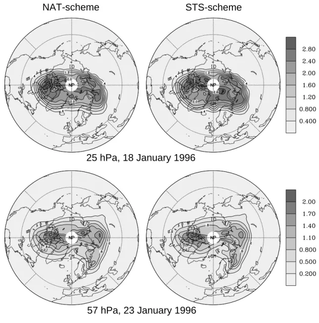
mid-NAT-scheme
STS-scheme
25 hPa, 18 January 1996
57 hPa, 23 January 1996
ClO [ ppbv ]
x
Fig. 7. ClOx(:=Cl+ClO+2 Cl2O2+2 Cl2+HOCl+OClO) mixing ratio (ppbv) modelled for (top frames) the 25 hPa and (bottom frames) the
57 hPa levels. Results are shown for two selected days of January 1996 showing comparatively large chlorine activation (57 hPa level on 23 January 1996, and 25 hPa level on 18 January 1996). The left frames and right frames show data modelled applying the NAT- and the STS-scheme, respectively.
January period of maximum chlorine activation are displayed in Fig. 7. Both Figs. 6 and 7 reveal that the ClOx
concen-trations obtained using the different PSC schemes can dif-fer significantly. Maximum deviations in spatial mean ClOx
(Fig. 6) amount to 0.1 ppbv. Local differences (Fig. 7) up to 0.3 ppbv (57 hPa) and 0.4 ppbv (25 hPa) occur during the January period of maximum activation. Similar to the simu-lations of Massie et al. (2000), the most effective early winter chlorine activation is modelled with the NAT-scheme. This partly changes during January and late February, especially during the periods of very low temperatures at 25 hPa when
very high liquid particle surface area concentrations occurred in the STS-scheme experiment (see also discussion on ozone changes). It should be noted that, apart from these differ-ences, the similarity between the different simulations is re-markable regarding the large contrasts in surface area con-centrations modelled with the NAT- and the STS-scheme. An important reason for this is the compensation between two important effects which were already discussed by Carslaw et al. (1997): On the one hand, the most relevant heteroge-neous reactions, especially ClONO2+HCl, are faster on
On the other hand, large surface area concentrations of liq-uid particles in the STS simulation are less frequent and are restricted to smaller areas when compared to the NAT sur-face area concentrations in the NAT-scheme case. It should be further noted that, in addition to PSC particles, binary sul-fate aerosols also have the potential to induce strong chlorine activation. This is indicated by the BIN-scheme simulation and agrees with the work of Massie et al. (2000). Consistent with the above discussion on the modelled PSC surface area concentrations, the chlorine activation simulated for Decem-ber and February using the STS/NAT-scheme is very similar to that modelled in the STS case. Due to the formation of solid particles in the STS/NAT simulation, the two scenarios diverge during January.
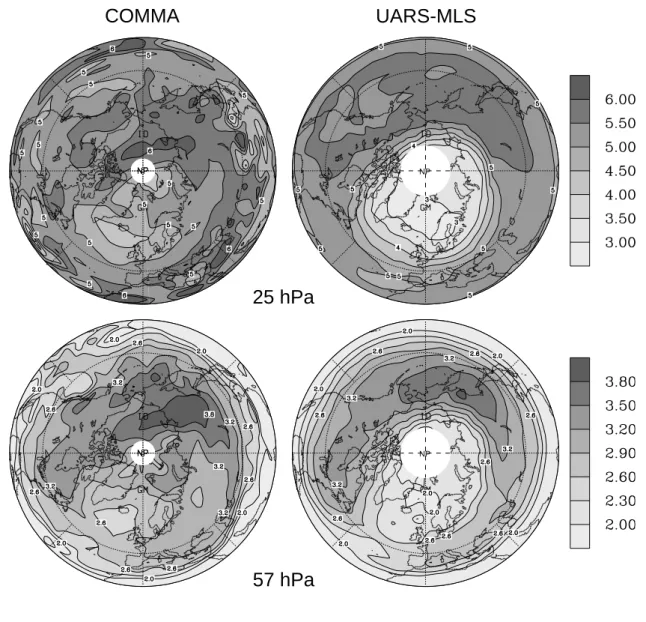
In order to assess the model quality with respect to the representation of stratospheric ozone distributions, we also compared the modelled ozone concentrations with UARS-MLS data. Due to the comparatively long lifetime of ozone, the spatial structure of the model ozone fields is likely to be sensitive to model deficiencies, such as potential short-comings in the representation of longer term trace gas trans-port. Hence, we compared modelled horizontal ozone distri-butions to corresponding MLS ozone fields. Since cumula-tive ozone loss is of particular relevance to polar stratospheric ozone depletion, special focus was given to the February ozone minimum which followed the strong January chlorine activation (Figs. 6 and 9). In order to evaluate the model quality for more than individual days, horizontal ozone dis-tributions were averaged over a time period starting on 13 February, which is the first day with data available after the MLS turn-off from 2 to 12 February. Since the comparison is primarily addressing the assessment of minimum ozone con-centrations, the averaging period ends on 20 February, which is the last day which is not impacted by model ozone recov-ery (see Fig. 9). Figure 8 shows the temporally averaged spatial distributions of ozone at 57 hPa and 25 hPa calcu-lated from the model output (STS/NAT case) and the MLS data, respectively. The comparison reveals that model ozone deviates from the observations especially in the polar vor-tex area. While the ozone maximum covering the North Pa-cific and Northeast Asia is well represented in the simulation with only slightly larger concentrations and a slight north-ward shift compared to the MLS data, the model overpre-dicts the ozone abundance within the polar vortex. The devi-ation of the modelled polar vortex ozone concentrdevi-ations from the corresponding MLS values typically ranges between 30% and 80% at 25 hPa, and between 20% and 50% at 57 hPa. These discrepancies exceed the MLS error which amounts to 10–20% within the lower stratosphere. The overprediction of polar vortex ozone appears to be a common problem of stratospheric 3-D models and was discussed in many previ-ous studies on ozone depletion in the Arctic winter strato-sphere (e.g. Steil et al., 1998; Hansen and Chipperfield, 1999; Ruhnke et al., 1999). Potential reasons for this effect are possible underrepresentations of PSC processes in strato-spheric models (e.g. the neglect of lee wave PSC (Hansen and Chipperfield, 1999) or the underestimation of
denitri-fication (Sinnhuber et al., 2000)) as well as deficiencies of current global stratospheric 3-D models concerning the rep-resentation of vertical transport, especially inside the vortex (Steil et al., 1998). As introduced above, the present study is intended to provide a sensitivity analysis of the impact of the differences in PSC schemes on model stratospheric chem-istry. Since the effect of ozone concentration on PSC mi-crophysics and on the efficiency of the related heterogeneous reactions is small, the impact of overestimations in model ozone should not affect the general conclusions on the sensi-tivities considered.
The temporal development of the PSC-induced ozone change at 57 and 25 hPa, averaged over the model domain north of 45◦N is highlighted in Fig. 9. In order to cap-ture only the PSC effects, the ozone change was calculated from the differences between the NAT-, the STS-, and the STS/NAT-scheme simulations, respectively, and the model experiment only considering liquid binary sulfate aerosols (BIN-scheme). Ozone changes in the range of −0.02 to
−0.04 ppmv calculated for the end of the simulated period
appear to be small, due to the fact that the values are aver-aged over a domain which is only partially affected by ozone loss (local PSC-induced ozone deficits of up to 0.2 ppmv are simulated). Another important reason is that ozone loss also occurs in the reference simulation including only binary sul-fate aerosols (BIN-scheme).
A significant scattering in the spatial mean ozone change resulting from the differences in the PSC-schemes is mod-elled. Maximum deviations of around 10 ppbv are simulated for mid-February. Apart from the conditions in late February at 25 hPa, the strongest ozone depletion is simulated in the case of the NAT-scheme experiment. This is due to the com-paratively high December temperatures and the correspond-ing lack of large liquid particle surface area concentrations occuring in the STS- and the STS/NAT-scheme experiments when effective NAT particle formation already takes place in the NAT-scheme simulation. The consequence is a de-lay in chlorine activation and the resulting ozone loss in the liquid particle cases, which can also be found in the results of Br¨uhl et al. (1997) obtained for the winter 1995/96. Due to similar conditions, ozone depletion rates modelled in the NAT-scheme experiment again exceed those of the STS- and the STS/NAT-scheme simulations in the beginning of Febru-ary. As discussed above (see discussion on Fig. 3), signif-icant solid particle occurrences in the STS/NAT case can be found only during January at 25 hPa. Hence, chlorine activation and the related ozone loss rates in the STS- and the STS/NAT-scheme experiments are nearly identical during December and February. Due to the January solid particle oc-currence, the STS/NAT-scheme simulation shows a smaller ozone depletion rate compared to the STS case, especially during the second half of January. Hence, the STS/NAT sim-ulation generally shows the smallest ozone depletion rather than representing an intermediate state between the STS- and the NAT-scheme model runs.
In mid-February, very low temperatures occurring at 25 hPa promote an increase in the liquid particle surface
COMMA
UARS-MLS
25 hPa
57 hPa
O [ ppmv ], 13 - 20 February 1996
3
NP NPFig. 8. Temporal mean ozone mixing ratio (ppmv) of the period between 13 and 20 February 1996, (left) calculated from the simulation using
the STS/NAT-scheme and (right) derived from UARS-MLS data. Horizontal distributions are shown for (top frames) 25 hPa and (bottom frames) 57 hPa.
area concentration and the related chlorine activation in the STS experiment (Figs. 3 and 6, top panels). This tempera-ture decrease was not strong enough to cause effective ice formation in the NAT-scheme experiment, as was the case during the January periods of large liquid surface area occur-rences. This results in a chlorine activation modelled with the STS-scheme largely exceeding that obtained using the NAT-scheme. As a consequence, late February ozone depletion at 25 hPa modelled in the STS-scheme simulation increases to be slightly larger when compared to the NAT-scheme experi-ment. As already mentioned, February ozone depletion rates behave similarly in the STS/NAT case and the STS simula-tion. However, for the reasons discussed above, the resulting PSC-induced ozone deficit in the STS/NAT case does not ex-ceed that modelled in the NAT-scheme simulation.
It should be noted that the assumptions on freezing con-ditions strongly impact the STS/NAT-scheme experiment. A threshold temperature of 3 K below the ice frost point is assumed for initial solid particle formation via freezing of liquid ternary solution droplets (Sect. 2.3). A higher freezing temperature may shift the results obtained with the STS/NAT-scheme towards those of the NAT-scheme simu-lation, as was the case in the Sessler et al. (1996) study. It should also be noted that the rate coefficients for het-erogeneous reactions on NAT are calculated here following “scheme 1” suggested by Carslaw et al. (1997). The cor-responding uptake coefficients can be taken as upper limits. Carslaw et al. also proposed a set of minimum likely up-take coefficients (“scheme 2”) which was not up-taken into ac-count here because, as pointed out in the Carslaw et al., study,
Figure 9
Fig. 9. Temporal change of the PSC-induced depletion of the ozone
mixing ratio (ppmv) averaged over the area north of 45◦N on the
model levels (bottom frame) 57 hPa and (top frame) 25 hPa. Re-sults are presented for the time period between 10 December 1995, and 29 February 1996, calculated from the differences between the model experiments performed with the NAT-, the STS- and the STS/NAT-scheme, respectively, and the simulation where only liq-uid binary sulfate aerosols are considered (BIN-scheme).
ozone depletion in the winter 1994/95 predicted on the basis of these coefficients, is less than that estimated from obser-vations. An application of “scheme 2” in the present simu-lations may shift the results of the NAT-scheme simulation obtained for the December to mid-February period towards those of the STS-scheme experiment.
Horizontal distributions of ozone differences between the NAT-scheme model run and the STS-scheme simulation, as calculated for the 57 hPa and the 25 hPa pressure levels, are presented in Fig. 10. The results are shown for 13 February, when the effective ozone depletion induced by the large Jan-uary chlorine activation has fully developed (Figs. 6 and 9), and for 25 February, when the spatial mean ozone deficit in the STS simulation exceeds that of the NAT-scheme exper-iment at 25 hPa (Fig. 9). Regarding 13 February, applica-tion of the NAT-scheme results in up to 20 ppbv lower ozone concentrations at both pressure levels when compared to the STS-scheme experiment. The maximum difference at 57 hPa decreases to values around 15 ppbv on 25 February. Never-theless, for the reasons discussed above, the difference be-tween the two experiments is of opposite sign on 25 Febru-ary at 25 hPa. Ozone depletion modelled in the STS-scheme simulation exceeds that calculated in the NAT experiment by typically around 15 ppbv and locally up to 40 ppbv. This in-crease in ozone depletion in the STS case is the response to
more than 1 ppbv larger mid-February ClOxconcentrations
(not displayed) in the STS-scheme simulation when com-pared to the NAT-scheme experiment. Also the trajectory cal-culations of Br¨uhl et al. (1997) suggest such an overturning in ozone depletion occurring in February 1996 in the Arctic stratosphere. Br¨uhl et al. (1997) modelled strong similarities in ozone loss in the liquid and the solid particle scenarios occurring until mid-February. In late February, ozone deple-tion in the liquid particle case exceeds that modelled when PSC particles are assumed to be solid. The ozone difference between these two model runs amounts to about 100 ppbv at the end of February. Thus a larger difference is modelled when compared to the present study. However, it should be mentioned that the trajectory assumed by Br¨uhl et al. (1997) is located somewhere in between the 25 hPa and the 57 hPa pressure levels considered in this study. Hence, the results of the trajectory calculations cannot directly be compared to the 3-D simulations performed here. Br¨uhl et al. (1997) also emphasized that the results obtained with the assumption of idealized trajectories have to be taken as qualitative. Further-more, discrepancies between trajectory calculations and 3-D model results can also be a consequence of the 3-D model deficiencies in vertical transport representation which were discussed above.
4 Conclusions
Simulations with a 3-D model were performed in order to investigate the impact of differences in PSC-microphysical schemes on the model chemistry of the winter Arctic strato-sphere. The model calculations were carried out for the win-ter 1995/96. Results obtained for the model levels located at 57 and 25 hPa were analysed. A comparison of simu-lations with a “NAT-scheme” and an “STS-scheme”, where PSC particles are considered to be solid or liquid, respec-tively, suggests that, in the considered winter, areas where NAT and other solid particles could potentially exist in equi-librium (T < TNAT) were significantly larger and occurred
over longer time periods compared to the areas showing con-ditions appropriate for large liquid particle formation. These differences induce significant deviations in chlorine activa-tion and the resulting ozone depleactiva-tion modelled assuming the different PSC microphysical schemes. At maximum chlorine activation, which is modelled for January 1996, local devia-tions in ClOx range up to 0.4 ppbv. At 57 hPa, the
NAT-scheme simulation shows larger maximum ClOx
concentra-tions compared to the STS-scheme case, and maximum chlo-rine activation levels in the STS-scheme experiment are pri-marily larger at 25 hPa. However, the PSC-induced mid-February ozone depletion resulting from the PSC activity during the mid-December to early February cold period is the largest in the solid particle case at both pressure levels. Even the corresponding ozone differences between the liquid and the solid particle experiments, which approach 20 ppbv, are quite similar at 25 and 57 hPa. These deviations in the mid-February ozone deficit are induced primarily by a temporal
57 hPa
25 hPa
13 February 1996
25 February 1996
∆
O [ ppbv ] (Difference: NAT-scheme
3
−
STS-scheme)
Fig. 10. Difference in the ozone mixing ratio (ppbv) occurring between the simulations performed with the NAT- and the STS-scheme on
(left) the 57 hPa and (right) the 25 hPa level. Results are presented obtained for (top panels) 13 February 1996, and (bottom panels) 25 February 1996.
delay in early winter chlorine activation in the STS case, caused by a lack of large liquid particle surface area concen-trations in December 1995. When NAT particles are already present in the NAT-scheme case, temperatures are still too high to allow for the effective growth of liquid particles in the STS-scheme simulation. The largest differences in chlo-rine activation occurring between the two model experiments develop in mid-February at pressure levels around 25 hPa. Over large areas, temperatures decrease below the threshold of effective liquid particle HNO3and water uptake. Due to
the resulting large liquid particle surface area concentrations and the very efficient heterogeneous chemistry on liquid par-ticles, effective chlorine activation occurs in the STS-scheme
simulation. Since temperatures fall infrequently below Tice
during mid-February and large NAT surface area concentra-tions are already present in the NAT-scheme experiment, a comparable increase in chlorine activation is not simulated in that case. Hence chlorine activation in the STS simulation strongly exceeds that modelled with the NAT-scheme. Max-imum local deviations in ClOxof up to 1.5 ppbv are
simu-lated. Consequently, ozone depletion is stronger in the STS model run under these conditions. For the end of February, maximum differences in the ozone mixing ratio of around 40 ppbv are modelled.
It should be noted that these differences in ozone concen-tration are significant but small relative to the large deviations
in PSC surface area concentrations modelled in the two ex-periments. This is primarily due to the larger efficiency of the most relevant heterogeneous reactions on liquids when compared to NAT. This compensates for the smaller mean surface area concentrations of liquid PSCs. It should be fur-ther noted that the STS/NAT simulation, where solid as well as liquid PSCs can occur, does not generally represent an in-termediate state between the STS- and the NAT-scheme ex-periments. The deviations of the STS/NAT simulation from the two other model runs are primarily controlled by the as-sumptions on freezing conditions. Thus, the freezing thresh-old temperature appears to be an important parameter which influences modelled stratospheric ozone depletion.
The results described above corroborate the findings of Br¨uhl et al. (1997), who investigated stratospheric ozone de-pletion in the winter 1995/96 by means of trajectory-box-model calculations. Our general conclusions are also con-sistent with the trajectory-box simulations of other winters performed by Br¨uhl et al. (1997) and Carslaw et al. (1997). However, maximum differences in ozone depletion caused by the assumptions about PSC particles being either liquid or solid are smaller in the 3-D simulations compared to the other studies.
In summary, differences in PSC-schemes can result in significant deviations in PSC-induced ozone depletion in the winter Arctic stratosphere simulated with stratospheric chemistry models. The largest differences between ozone depletion modelled assuming liquid or solid PSCs, respec-tively, can be expected when the following conditions can be encountered on large spatial scales and for prolonged time periods in the winter Arctic stratosphere. First, stratospheric temperatures stay below TNATbut above the threshold of
ef-fective liquid particle growth. Second, temperatures stay sig-nificantly below this threshold but do not fall below the ice frost point.
Acknowledgement. We want to express our thanks to G. Brasseur
(NCAR, now at MPI-M) for supplying the programs for precal-culating the look-up table of photolysis rates. We are grateful to
D. K. Weisenstein (AER Inc.) for providing AER 2-D data of Bry
and Clyconcentrations. The UARS-MLS data was supplied by the
British Atmospheric Data Centre (BADC) and the Jet Propulsion Laboratory (JPL). European Centre for Medium Range Weather Forecasts (ECMWF) global analysis data were used with permis-sion of the German Weather Service (DWD). The present study was financially supported by the German Federal Ministry for Educa-tion, Science, Research and Technology (BMBF) under grant 01 LO9516/3. Computational support was provided by the Regional Computing Centre (RRZK) of the University of Cologne.
Topical Editor D. Murtagh thanks M. Santee and another referee for their help in evaluating this paper.
References
Abbatt, J. P. D. and Molina, M. J., The heterogeneous reaction of
HOCl + HCl → Cl2 + H2O on ice and nitric acid trihydrate:
reaction probabilities and stratospheric implications, Geophys. Res. Lett., 19, 461–464, 1992.
Baier, F., Entwicklung und Anwendung eines adjungierten Modells zur Simulation des Ozonhaushaltes der Stratosph¨are w¨ahrend realer Episoden, in Mitteilungen aus dem Institut f¨ur Geophysik und Meteorologie der Universit¨at zu K¨oln, (Eds) Kerschgens, M., Neubauer, F. M., P¨atzold, M., Speth, P., and Tezkan, B., ISSN 0069–5882, 141, 154, K¨oln, Germany, 2000.
Baulch, D. L., Duxbury, J., Grant, S. J., and Montague, D. C., Eval-uated kinetic Data for high temperature reactions, Vol. 4, Homo-geneous Gas Phase Reactions of Halogen and Cyanide Contain-ing Species, J. Phys. Chem. Ref. Data, 10, Suppl. 1, 721, 1981. Berger, U. and Dameris, M., Cooling of the upper atmosphere due
to CO2increase: a model study, Ann. Geophysicae, 11, 809–819,
1993.
Berger, U. and Ebel, A., Dependence of the energy budget at mesopause heights on variable circulation patterns, Adv. Space. Res., 17, 111–116, 1995.
Berger, U. and von Zahn, U., The two-level structure of the mesopause: A model study, J. Geophys. Res., 104, 22 083– 22 093, 1999.
Biele, J., Neuber, R., Warming, J., Beninga, I., von der Gathen, P., Stebel, K., Schrems, O., and Rosen, J., The evolution of polar stratospheric clouds above Spitzbergen in winter 1996/97, in Po-lar Stratospheric Ozone 1997, Proceedings of the 4th European Symposium, 22 to 26 September 1997, Schliersee, Bavaria, Ger-many, (Eds) Harris, N. R. P., Kilbane-Dawe, I., and Amanatidis, G. T., European Communities, Luxembourg, 99–102, 1998. Bott, A., Monotone flux limitation in the area-preserving flux-form
advection algorithm, Mon. Wea. Rev., 120, 2592–2602, 1992. Brasseur, G., Hitchman, M. H., Walters, S., Dymek, M., Falise, E.,
and Pirre, M., An interactive chemical dynamical radiative two-dimensional model of the middle atmosphere, J. Geophys. Res., 95, 5639–5655, 1990.
Browell, E. V., Buttler, C. F., Ismail, S., Robinette, P. A., Carter, A. F., Higdon, N. S., Toon, O. B., Schoeberl, M. R., and Tuck, A. F., Airborne lidar observations in the wintertime Arctic strato-sphere: polar stratospheric clouds, Geophys. Res. Lett., 17, 385– 388, 1990.
Br¨uhl, C., Carslaw, K., Peter, T., Grooß, J.-U., Russel III, J. M., and M¨uller, R., Chlorine activation and ozone depletion in the Arctic vortex of the four recent winters using a trajectory box model and HALOE satellite observations, in Proc. XVIII Quadrennial Ozona Symp., L’Aquila, 12–21 September 1996, 675–678, 1997. Burkholder, J. B., Talukdar, R. K., and Ravishankara, A. R.,
Tem-perature dependence of the ClONO2 UV absorption spectrum.
Geophys. Res. Lett., 21, 585–588, 1994.
Carslaw, K. S., Luo, B. P., Clegg, S. L., Peter, T., Brimblecombe, P.,
and Crutzen, P. J., Stratospheric aerosol growth and HNO3gas
phase depletion from coupled HNO3and water uptake by liquid
particles, Geophys. Res. Lett., 21, 2479–2482, 1994.
Carslaw, K. S., Luo, L., and Peter, T., An analytic expression for the composition of aqueous HNO3-H2SO4stratospheric aerosols
including gas phase removal of HNO3, Geophys. Res. Lett., 22,
1877–1880, 1995.
Carslaw, K. S., Peter, T., and M¨uller, R., Uncertainties in reactive uptake coefficients for solid stratospheric particles–2. Effect on ozone depletion, Geophys. Res. Lett., 24, 1747–1750, 1997. Carslaw, K. S., Peter, T., Bacmeister, J. T., and Eckermann, S. D.,
Widespread solid particle formation by mountain waves in the Arctic stratosphere, J. Geophys. Res., 104, 1827–1836, 1999. Dameris, M., Berger, U., G¨unther, G., and Ebel, A., The ozone hole:
dynamical consequences as simulated with a three-dimensional model of the middle atmosphere, Ann. Geophysicae, 9, 661–668,