HAL Id: insu-01696520
https://hal-insu.archives-ouvertes.fr/insu-01696520
Submitted on 26 Apr 2019
HAL is a multi-disciplinary open access
archive for the deposit and dissemination of
sci-entific research documents, whether they are
pub-lished or not. The documents may come from
teaching and research institutions in France or
abroad, or from public or private research centers.
L’archive ouverte pluridisciplinaire HAL, est
destinée au dépôt et à la diffusion de documents
scientifiques de niveau recherche, publiés ou non,
émanant des établissements d’enseignement et de
recherche français ou étrangers, des laboratoires
publics ou privés.
Top-down CO emissions based on IASI observations and
hemispheric constraints on OH levels
Jean-François Müller, Trissevgeni Stavrakou, Maite Bauwens, Maya George,
Daniel Hurtmans, Pierre-François Coheur, Cathy Clerbaux, Colm Sweeney
To cite this version:
Jean-François Müller, Trissevgeni Stavrakou, Maite Bauwens, Maya George, Daniel Hurtmans, et
al..
Top-down CO emissions based on IASI observations and hemispheric constraints on OH
levels.
Geophysical Research Letters, American Geophysical Union, 2018, 45 (3), pp.1621-1629.
Geophysical Research Letters
Top-Down CO Emissions Based On IASI Observations
and Hemispheric Constraints on OH Levels
J.-F. Müller1 , T. Stavrakou1, M. Bauwens1, M. George2, D. Hurtmans3, P.-F. Coheur3 , C. Clerbaux2,3 , and C. Sweeney4
1Royal Belgian Institute for Space Aeronomy, Brussels, Belgium,2LATMOS/IPSL, UPMC University Paris 06 Sorbonne
Universités, UVSQ, CNRS, Paris, France,3Atmospheric Spectroscopy, Service de Chimie Quantique et Photophysique,
Université Libre de Bruxelles (ULB), Brussels, Belgium,4NOAA Earth System Research Laboratory, Boulder, Colorado, USA
Abstract
Assessments of carbon monoxide emissions through inverse modeling are dependent on the modeled abundance of the hydroxyl radical (OH) which controls both the primary sink of CO and its photochemical source through hydrocarbon oxidation. However, most chemistry transport models (CTMs) fall short of reproducing constraints on hemispherically averaged OH levels derived from methylchloroform (MCF) observations. Here we construct five different OH fields compatible with MCF-based analyses, and we prescribe those fields in a global CTM to infer CO fluxes based on Infrared Atmospheric Sounding Interferometer (IASI) CO columns. Each OH field leads to a different set of optimized emissions. Comparisons with independent data (surface, ground-based remotely sensed, aircraft) indicate that the inversion adopting the lowest average OH level in the Northern Hemisphere (7.8 × 10⁵molec cm−3, ∼18% lowerthan the best estimate based on MCF measurements) provides the best overall agreement with all tested observation data sets.
Plain Language Summary
Satellite measurements of a pollutant can be used to deduce the emissions of this pollutant to the atmosphere. But often, such estimates have errors due to our uncertain knowledge of the chemical lifetime of pollutants. Here we assess the importance of specifying the correct lifetime for deducing the sources of carbon monoxide. We also show that the measurements can provide new constraints on the lifetime of pollutants. More precisely, we provide constraints on the abundance of OH radicals, often considered to be the main detergent of the atmosphere. Indeed, OH radical is the main oxidant of carbon monoxide, but also methane, which is a potent greenhouse gas.1. Introduction
The sources of CO include direct emissions and photochemical production due to the oxidation of hydrocar-bons. The dominant CO sink being its reaction with the hydroxyl radical (OH), CO has a strong influence on the oxidative capacity of the atmosphere and on the removal of air pollutants. Previous modeling studies used CO measurements in combination with chemistry-transport models (CTMs) to provide top-down constraints on the surface emissions and (in some cases) also the photochemical production of CO (Fortems-Cheiney et al., 2009, 2011; Jiang et al., 2015, 2017; Kopacz et al., 2010; Stavrakou & Müller, 2006). The resulting updated emis-sions are sensitive not only to the choice of atmospheric data set and inversion setup but also to the modeled OH abundance, primarily because reaction with OH is by far the largest CO sink (also because methane oxida-tion by OH is among the largest CO sources) (Kopacz et al., 2010; Stavrakou & Müller, 2006). Model-calculated OH fields show large differences among models; for example, the global tropospheric chemical lifetime of methane ranges between 7.1 and 13.9 years (Voulgarakis et al., 2013), whereas the best estimate based on methylchloroform (MCF) is 11.2 years with an uncertainty range of 9.8–12.5 years (Prather et al., 2012). Fur-thermore, while models predict higher OH in the Northern than in the Southern Hemisphere, a recent MCF analysis (Patra et al., 2014) indicate an interhemispheric N/S ratio (RNS) very close to 1 (0.97±0.12), much lower
than the Atmospheric Chemistry and Climate Model Intercomparison Project (ACCMIP) multimodel mean ratio of 1.28 ± 0.10 (Naik et al., 2013). The OH levels being overestimated by most models in the Northern Hemisphere, the total hemispheric top-down CO emissions are likely too high. Here we conduct an inverse modeling assessment of the global CO budget based on Infrared Atmospheric Sounding Interferometer (IASI) retrievals (George et al., 2015) for 2013, taking into account the MCF-derived constraints on global and
RESEARCH LETTER
10.1002/2017GL076697 Key Points:
• The global CO sources were inferred based on IASI CO columns, using a global CTM and prescribed OH fields • Varying hemispheric mean OH levels within their uncertainties estimated from methylchloroform analyses has a strong impact on derived fluxes • The inversion adopting the lowest OH
in NH provides the best match with satellite, in situ, and FTIR data
Supporting Information: • Supporting Information S1 Correspondence to: J.-F. Müller, [email protected] Citation:
Müller, J.-F., Stavrakou, T., Bauwens, M., George, M., Hurtmans, D., Coheur, P.-F., Clerbaux, C., & Sweeney, C. (2018). Top-down CO emissions based on IASI observations and hemispheric constraints on OH levels. Geophysical Research Letters, 45, 1621–1629. https://doi.org/10.1002/2017GL076697
Received 8 DEC 2017 Accepted 21 JAN 2018
Accepted article online 29 JAN 2018 Published online 2 FEB 2018
©2018. The Authors.
This is an open access article under the terms of the Creative Commons Attribution-NonCommercial-NoDerivs License, which permits use and distribution in any medium, provided the original work is properly cited, the use is non-commercial and no modifications or adaptations are made.
Geophysical Research Letters
10.1002/2017GL076697
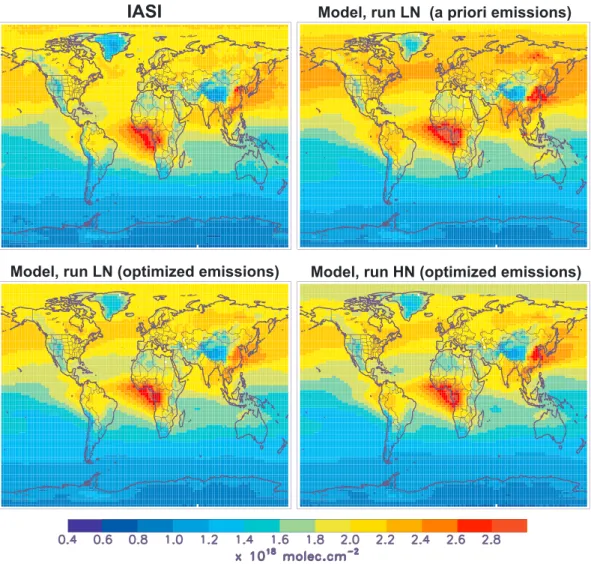
Figure 1. Annually averaged CO columns observed by (top left) Infrared Atmospheric Sounding Interferometer (IASI) in
2013, and modeled with IMAGES using (top right) a priori or (bottom panels) optimized emissions. The LN (low OH in Northern Hemisphere) and HN (high OH in NH) runs refer to the OH fields used in the model (Table 1).
hemispheric mean OH levels. Sensitivity inversions are performed to estimate the impact of OH level uncer-tainties, and comparisons with in situ, ground-based, remote-sensed, and aircraft data are conducted to evaluate the results.
2. Methods
2.1. IMAGES
The IMAGES model (Bauwens et al., 2016; Stavrakou et al., 2016) calculates the distribution of 170 chem-ical compounds at 2∘ × 2.5∘ resolution between the surface and the lower stratosphere (44 hPa) using ERA-Interim ECMWF meteorology (Dee et al., 2011). The model uses anthropogenic emissions from HTAPv2 (Janssens-Maenhout et al., 2015), with the nonmethane volatile organic compounds (NMVOC) speciation provided by ACCMIP (Lamarque et al., 2010), fire emissions from GFED4s (van der Werf et al., 2017), and bio-genic VOC emissions calculated using MEGAN-MOHYCAN (Guenther et al., 2006; Müller et al., 2008; Stavrakou et al., 2011). Biogenic CO emissions and CO deposition are also taken into account (Müller & Stavrakou, 2005). The chemical degradation mechanism is described in Bauwens et al. (2016) and includes recent isoprene mechanism updates as well as an explicit treatment for 16 other NMVOCs. To minimize the impact of model errors associated with stratospheric chemistry and the boundary condition at the model top, the CO mixing ratios in the seven uppermost layers (44, 55, 67, 80, 96, 113, and 133 hPa) are fixed and set to a reanalysis of Aura Microwave Limb Sounder observations (Santee et al., 2017) by the Belgian Assimilation System for Chemical Observations stratospheric assimilation system (Errera et al. (2017), Figure S1). The flux inversion
Geophysical Research Letters
10.1002/2017GL076697
Table 1
Description of OH Fields Used in the CO Inversions 𝜏OH
CH4 [OH] in NH [OH] in SH
Run label Description (years) RNS (105cm−3) (105cm−3)
STD Standard 11.2 0.97 9.2 9.5
HN Very high OH in NH 9.8 1.10 11.2 10.1 LN Very low OH in NH 12.5 0.85 7.8 9.0 HS Very high OH in SH 9.8 0.85 9.8 11.5 LS Very low OH in SH 12.5 1.10 8.8 8.0
Note. The parameter𝜏OH
CH4denotes the tropospheric chemical lifetime of methane,RNSis the
interhemispheric ratio.
methodology is based on the adjoint of IMAGES (Stavrakou & Müller, 2006) with a few adaptations briefly discussed in the supporting information.
2.2. IASI Observations
The observations are monthly averaged CO total columns from IASI on board Metop-A (Clerbaux et al., 2009; Hurtmans et al., 2012) for 2013 binned onto the CTM resolution (Figures 1, and S2). IASI provides a global cov-erage twice daily. IASI CO data were previously used in modeling studies (e.g., Fortems-Cheiney et al., 2009; Klonecki et al., 2012) and evaluated against other satellite data sets (George et al., 2009, 2015). The instrument sensitivity is highest in the middle to upper troposphere. Since the vertical information content is coarse, the profiles are not used in the inversion. The model accounts for the IASI averaging kernels and for the tempo-ral sampling in the monthly averages. Since the information content is low at high latitudes during winter, due to the low temperatures and low signal-to-noise ratio (Pommier et al., 2010), we exclude the winter months, defined by the following: October–May (>75∘N), November–April (65–75∘ N), November–March (55–65∘ N), November–February (48–55∘ N), and similarly in the Southern Hemisphere (shifted by 6 months). This definition was guided by comparisons with Fourier-transform infrared spectroscopy (FTIR) total column data (Figure S3, S4).
The IASI total error (sum of measurement and smoothing error) is typically very low (2–5%) over continents during summer and somewhat higher (5–15%) elsewhere. The number of data per model grid cell and per month is generally very high (200–2,000) and only the systematic part of the retrieval error contributes non-negligibly to the measurement error of the superobservations, namely, the monthly averaged columns at 2∘ × 2.5∘. The large number of measurements per superobservation also reduces greatly the representativity error associated with CO variability within the same grid cell and month (Miyazaki et al., 2012). The dominant error component is the CTM error, which is more difficult to assess. It is here taken to be 35% of the CO column. This choice is supported by the𝜒2diagnostic (i.e., the first term of the cost function divided by the number
of observations, cf. supporting information), which should be close to one after optimization (Klonecki et al., 2012). As discussed below its value is of the order of 0.8 after optimization.
2.3. OH Fields Used in CO Inversions
The OH concentrations simulated by IMAGES are replaced in the troposphere by distributions in line with observational constraints based on MCF observations (Patra et al., 2014; Prather et al., 2012). The OH fields rely on the climatological tropospheric distributions of Spivakovsky et al. (2000) (S2000) adjusted to match the MCF constraints. The S2000 distribution achieves RNS≈ 1, with hemispherically averaged OH concentrations [OH]NH = 11.4 × 105cm−3and [OH]
SH = 11.5 × 105cm−3and it implies a global tropospheric chemical
methane lifetime of 9.1 years. This field is scaled in each hemisphere to match the hemispherically averaged OH concentrations (Table 1) calculated using
[OH]NH= Xg 2 RNS RNS+ 1 , [OH]SH= Xg 2 RNS+ 1 (1) where Xgis the globally averaged OH concentration consistent with Prather et al. (2012) (best value: 0.932 ×
106cm−3, uncertainty range = (0.835 − 1.065)106cm−3), and R
NSthe N/S concentration ratio from Patra et al.
Geophysical Research Letters
10.1002/2017GL076697
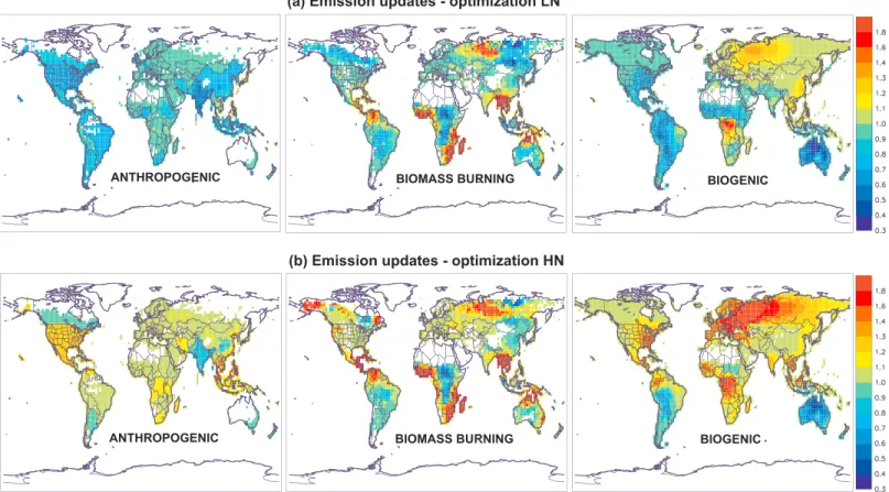
Figure 2. Annually averaged emission updates (ratios (optimized fluxes)/(a priori fluxes)) for the three source categories (anthropogenic, biomass burning, and
biogenic) in the optimization (a) HN and (b) LN.
3. Results
3.1. Optimized Fluxes
The IASI CO columns are illustrated on Figure 1 along with the IMAGES CO columns with either a priori or opti-mized emissions. In contrast with previous modeling studies (Fortems-Cheiney et al., 2009; Kopacz et al., 2010; Stavrakou & Müller, 2006), the modeled columns of the LN simulation overestimate the observations over most of the Northern Hemisphere, due to the lower OH concentrations and therefore higher CO lifetime com-pared to those studies. The optimizations bring the model much closer to IASI data (Figure S5); for example, the𝜒2diagnostic (which measures the overall bias between model and observations) is reduced by almost
65% in both hemispheres in the LN optimization. Among the different optimizations, LN achieves the lowest average𝜒2(0.70), followed by LS and the standard run STD (both 0.74), whereas the optimizations with higher
OH (HN and HS) performed comparatively worse (0.86 and 0.84). The LN inversion is also the simulation which achieves the lowest mean bias in both hemispheres (−0.1% in NH and 0.2% in SH).
Although the major features of the optimized model CO columns are similar in all five source inversions (Figure 1), the corresponding top-down emission estimates show large differences (Figure 2 and Table 2), in particular, for anthropogenic emissions (factor of 1.4 between global emissions in HN and LN). The higher (lower) OH levels in the HN (LN) inversion lead to a shorter (longer) CO lifetime, which is compensated by higher (lower) emissions. The inferred isoprene emissions are also strongly sensitive to the OH levels, and range between 353 (LN) and 454 Tg yr−1(HN).
The global fluxes range between 2,139 (in LN) and 2,711 Tg CO (in HN, Table 2) and are generally lower com-pared to previous estimates, for example, 2,748 Tg CO (Stavrakou & Müller, 2006), 2,857 Tg CO (Kopacz et al., 2010), and 2,391 Tg CO (Jiang et al., 2017). The latter study derived an annual anthropogenic flux of 54.3 Tg CO over the United States in 2013, at the upper end of our estimated range, but about half of a previous top-down estimate (97 Tg CO, Jiang et al. (2015)). Low anthropogenic CO emissions over the United States are supported by independent evaluations using aircraft data. Data collected during the aircraft campaign of the International Consortium for Atmospheric Research on Transport and Information in 2004 suggested
Geophysical Research Letters
10.1002/2017GL076697
Table 2
A Priori and Optimized CO Fluxes (Tg CO yr−1) in the Five Inversions (Table 1)
A priori STD HN LN HS LS Anthropogenic North America 66 61 79 50 66 58 USA 44 39 53 31 42 37 Europe 30 29 30 27 29 28 China 166 164 202 134 175 156 India 63 44 52 37 47 41 Global 544 511 617 436 564 478 Open fires North Africa 55 53 57 51 53 53 South Africa 95 107 113 102 120 96 Amazonia 16 15 15 14 17 12 Indonesia 17 10 10 9 10 9 Global 291 320 352 294 354 293
Other sources (global)
CH4+OH 718 718 820 644 816 648
NMVOC 750 733 815 674 813 671
Ocean/soils 96 98 107 91 108 90
Total source
Global 2399 2381 2711 2139 2655 2180
that the U.S. EPA (Environmental Protection Agency) overestimates CO emissions by 60% (Hudman et al., 2008), corresponding to an estimate of 26 Tg in 2013 when accounting for the emission trend (www.epa.gov/ sites/production/files/2016-12/national_tier1_caps.xlsx). Using a geographically more limited data set, another study deduced a 15% overestimation of U.S. EPA emissions, implying a flux of 42 Tg CO in 2013 (Anderson et al., 2014). The CO top-down estimate of the LN inversion (31 Tg yr−1) lies between these two campaign-based
estimates, whereas the U.S. total of the HN inversion (53 Tg yr−1) seems largely overestimated.
The annual top-down fluxes over China range between 134 Tg CO (LN) and 202 Tg CO (HN), in good agree-ment with a previous inversion based on Measureagree-ment Of Pollution in the Troposphere (MOPITT) columns (160–177 Tg CO; Jiang et al., 2017). It is difficult to further validate the CO emission inventories, especially in China, due to the sparcity of independent measurements. Estimates from different bottom-up invento-ries indicate large differences for the same year (2008), 105 Tg CO in EDGARv3.2 (European Commission Joint Research Centre, 2011), 202 Tg in REASv2.1 (Kurokawa et al., 2013), whereas recent evaluations suggest intermediate values (153 Tg in EDGARv4.3.1 and 158 Tg in Saikawa et al., 2017, both for 2008).
The sensitivity of the fire emissions to OH levels is relatively smaller (Table 2). However, all inversions indicate strongly decreased fluxes over Indonesia during the fire season, with the strongest decrease (factor of 3) occur-ring in June. This result is supported by an independent top-down inversion of VOC fluxes based on HCHO columns (Bauwens et al., 2016), pointing to a large flux overestimation (factor of 5) in the GFED4s database in this region in June 2013. Similarly, the inferred decrease in Amazonian fire fluxes is corroborated by a similar emission decrease in VOC fluxes in August–September 2013 (ca. 20%, Bauwens et al., 2016).
3.2. Comparison to Independent Observations
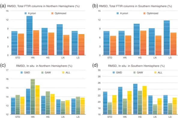
We evaluate the inversions against ground-based FTIR total CO columns at 16 sites of the Network for the Detection of Atmospheric Composition Change (NDACC) (ftp.cpc.ncep.noaa.gov/ndacc/station, see sup-porting information). Their estimated systematic errors are typically 2–4%. For simplicity, we focus on the inversions with either the lowest (LN) or the highest (HN) [OH] in the Northern Hemisphere, where most eval-uation data are available. In all simulations, the root-mean-square deviation (RMSD) between modeled and observed monthly columns is decreased in both hemispheres in the posterior estimates. The results in the Northern Hemisphere indicate a clear improvement when [OH] is low (RMSD of 6.9% for LN, 8.4% for HN). A large part (about half ) of the difference between the RMSD of LN and HN inversions is associated with
Geophysical Research Letters
10.1002/2017GL076697
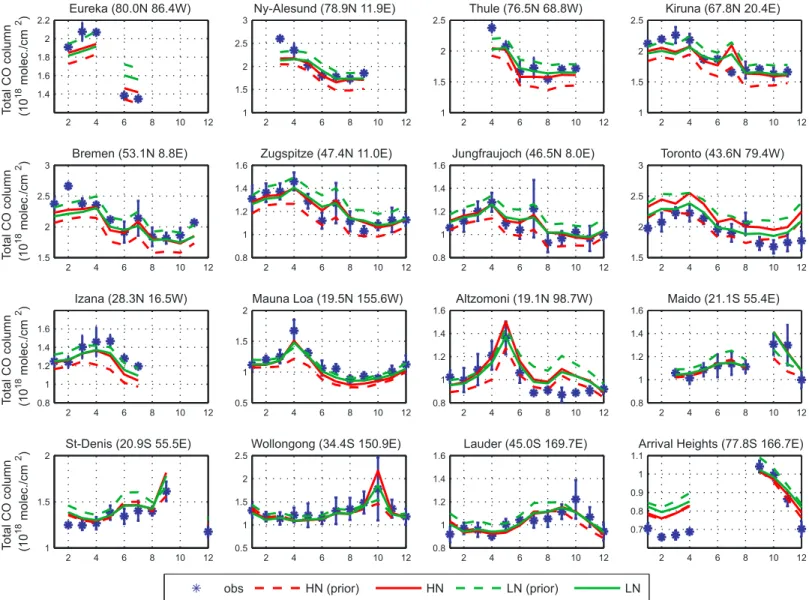
Figure 3. Modeled and observed CO columns at Fourier-transform infrared spectroscopy (FTIR) stations. In dark blue: FTIR monthly means with their standard
deviations; dashed lines: modeled values using a priori fluxes; solid lines: modeled values using optimized fluxes. HN run in red, LN in green.
the stations of Toronto and Mauna Loa. At Toronto, located in the direct vicinity of anthropogenic emission sources, the higher CO fluxes of the HN inversion lead to a significant overestimation (+10%, Figure 3). At Mauna Loa, far away from the source areas and where CO is therefore more sensitive to OH levels, HN underesti-mates the FTIR columns in spite of its higher emissions. The RMSD between the model and FTIR columns is very similar to the RMSD between the model and IASI columns (7.3% for LN, 8.3% for HN in the Northern Hemisphere), suggesting an excellent general consistency between IASI and FTIR CO total columns, at least when high-latitude wintertime IASI data are excluded. In the Southern Hemisphere, both FTIR and IASI data indicate a better agreement (lower RMSD) when OH levels are close to the standard case (runs STD, LN, HN, with RMSD very close to 6.6% against FTIR in all three cases) than when OH is either very high (HS, 8.3%) or very low (LS, 7.7%, Figure 4).
The optimizations are further evaluated against surface CO mixing ratios from the NOAA/GMD and GAW net-works (Figure S6), for a total of 90 stations providing data in 2013. The uncertainty on those measurements is typically 2–5 ppb (Novelli et al., 2017). The comparison is summarized in Figures 4 and S7. Overall, the best (worst) performance in the Northern Hemisphere is realized by the LN (HN) simulation. The LN simula-tion provides also the best match with Southern Hemisphere data. The RMSD is strongly decreased in the Southern Hemisphere upon inversion, for example, from 49 to 21% for LN. This is for largely due to the reduc-tion of fire emissions over Indonesia in June, causing a strong reducreduc-tion of the bias at Bukit Kotobatang in
Geophysical Research Letters
10.1002/2017GL076697
12 13 14 15 16 17 STD HN HS LN LS GMD GAW ALL 16 18 20 22 24 26 28 30 STD HN HS LN LS GMD GAW ALL 0 3 6 9 12 15 STD HN HS LN LS A priori Optimized 0 3 6 9 12 15 STD HN HS LN LS A priori OptimizedRMSD, Total FTIR columns in Northern Hemisphere (%) RMSD, Total FTIR columns in Southern Hemisphere (%)
) % ( e r e h p s i m e H n r e h t u o S n i u t i s n I , D S M R ) % ( e r e h p s i m e H n r e h t r o N n i u t i s n I , D S M R
(a)
(d)
(c)
(b)
Figure 4. (upper panels) RMSD (in %) between monthly Fourier-transform infrared spectroscopy (FTIR) CO total columns
and corresponding model values and (lower panels) between monthly CO mixing ratios at GMD/GAW stations and the optimized model fields in the (left) Northern and (right) Southern Hemispheres.
Sumatra (Figure S7). The RMSD reduction from optimization is smaller in the Northern Hemisphere (from 14.5 to 13.6%). The model generally underestimates the wintertime observations at high northern latitudes, pos-sibly due to the exclusion of high-latitude wintertime IASI data in the inversions. As for the FTIR total columns, the HN simulation overestimates CO over source areas (e.g., over Colorado and Utah) and it underestimates CO at remote oceanic sites (Midway, Mauna Loa and Guam), whereas the LN achieves a comparatively better match at these stations. The general conclusions are therefore consistent with those drawn from total CO col-umn data. Nevertheless, the comparisons for surface mixing ratios show a larger spread (reflected by larger RMSD) than in the case of total columns. This is likely due to the larger model uncertainties for surface mixing ratios than for total columns, which are less affected by errors associated with vertical mixing.
Finally, the modeled CO profiles over North America are evaluated against aircraft measurements from the SEAC4RS (Toon et al., 2016) and DC3 (Barth et al., 2015) campaigns and from the Global Greenhouse Gas
Ref-erence Network (GGGRN) (Sweeney et al., 2015) (cf. Figure S8). Despite their very different emissions and OH fields, the three optimizations yield very similar results in the middle and upper troposphere, where IASI sen-sitivity is highest (4–12 km). Closer to the surface, however, significant differences are found, reaching up to 20% between HN and LN. The higher emissions of the HN inversion lead to near-surface CO overestimation in all campaigns and (for GGGRN) at all seasons, although the discrepancy is very small in spring and fall. The LN achieves the best agreement (lowest RMSD) with observations of both DC3 and SEAC4RS campaigns, as well
as of GGGRN data in summer and winter, and it also performs better than the HN inversion against GGGRN data in spring and fall.
4. Discussion and Conclusions
This study demonstrates the strong impact of model uncertainties in OH concentrations on global and regional top-down CO flux estimates. For example, differences of 40% in the top-down global anthropogenic emissions are found when varying the OH levels, and even larger differences are found regionally, for example, over China and the United States. Clearly, all inverse modeling studies addressing CO, CH4, and other reactive species should report their global mean OH levels and interhemispheric ratios.
Evaluation of our results against IASI and a wide range of independent CO measurements (FTIR total columns, network surface mixing ratios, aircraft in situ data) shows that the inversion adopting the lowest average OH
Geophysical Research Letters
10.1002/2017GL076697
abundance in the Northern Hemisphere provides the best match with most observational sets, suggesting, in particular, that the interhemispheric (NH/SH) OH ratio might be close to the lower end of the range (0.85–1.1) reported by Patra et al. (2014), whereas the global photochemical methane lifetime might be near the upper end of the range (9.8–12.5 years) given in Prather et al. (2012). This inversion achieves the best agreement with measurements in the Southern Hemisphere, although other source inversions (e.g., STD) achieve very similar results in that hemisphere. While uncertainties exist due to errors in transport, seasonal evolution, and intra-hemispheric distributions of OH, we note that these inverse estimates fit independent aircraft measurements of the Eastern United States best assuming low OH in the Northern Hemisphere.
References
Anderson, D. C., Loughner, C. P., Diskin, G., Weinheimer, A., Canty, T. P., Salawitch, R. J.,…Disckerson, R. R. (2014). Measured and modeled CO and NOyin DISCOVER-AQ: An evaluation of emissions and chemistry over the eastern US. Atmospheric Environment, 96, 78–87.
Barth, M., Cantrell, C. A., Brune, W. H., Rutledge, S. A., Crawford, J. H., Huntrieser, H.,…Ziegler, C. (2015). The deep convective clouds and chemistry (DC3) field campaign. Bulletin of the American Meteorological Society, 96, 1281–1309.
Bauwens, M., Stavrakou, T., Müller, J.-F., De Smedt, I., Van Roozendael, M., van der Werf, G. R.,…Guenther, A. (2016). Nine years of global hydrocarbon emissions based on source inversion of OMI formaldehyde observations. Atmospheric Chemistry and Physics, 16, 10,133–10,158. https://doi.org/10.5194/acp-16-10133-2016
Clerbaux, C., Boynard, A., Clarisse, L., George, M., Hadji-Lazaro, J., Herbin, H.,…Coheur, P.-F. (2009). Monitoring of atmospheric composition using the thermal infrared IASI/MetOp sounder. Atmospheric Chemistry and Physics, 9, 6041–6054.
Dee, D., Uppala, S., Simmons, A., Berrisford, P., Poli, P., & Kobayashi, S. (2011). The ERA-Interim reanalysis: Configuration and performance of the data assimilation system. Quarterly Journal of the Royal Meteorological Society, 137(656), 553–597. https://doi.org/10.1002/qj.828 Errera, Q., Braathen, G., Chabrillat, S., Christophe, Y., Santee, M., & Skachko, S. (2017). BRAM: A reanalysis of Aura MLS chemical observations by
the Belgian Assimilation System for Chemical Observations (BASCOE). Vienna: European Geophysical Union (EGU) General Assembly. European Commission Joint Research Centre, JRC/Netherlands (2011). Emission Database for Global Atmospheric Research (EDGAR),
release version 4.2. Retrieved from http://edgar.jrc.ec.europa.eu last access: 28 April 2017
Fortems-Cheiney, A., Chevallier, F., Pison, I., Bousquet, P., Carouge, C., Clerbaux, C.,…Szopa, S (2009). On the capability of IASI measurements to inform about CO surface emissions. Atmospheric Chemistry and Physics, 9, 8735–8743.
Fortems-Cheiney, A., Chevallier, F., Pison, I., Bousquet, P., Szopa, S., Deeter, M. N., & Clerbaux, C. (2011). Ten years of CO emissions as seen from Measurements of Pollution in the Troposphere (MOPITT). Journal of Geophysical Research, 116, D05304. https://doi.org/10.1029/2010JD014416
George, M., Clerbaux, C., Bouarar, I., Coheur, P.-F., Deeter, M. N., Edwards, D. P.,…Worden, H. M. (2015). An examination of the long-term CO records from MOPITT and IASI: Comparison of retrieval methodology. Atmospheric Measurement Techniques, 8, 4313–4328. https://doi.org/10.5194/amt-8-4313-2015
George, M., Clerbaux, C., Hurtmans, D., Turquety, S., Coheur, P.-F., Pommier, M.,…McMillan, W. (2009). Carbon monoxide distributions from the IASI/METOP mission: Evaluation with other space-borne remote sensors. Atmospheric Chemistry and Physics, 9, 8317–8330. Guenther, A., Karl, T., Harley, T., Wiedinmyer, C., Palmer, P., & Geron, C. (2006). Estimates of global terrestrial isoprene emissions using MEGAN
(Model of Emissions of Gases and Aerosols from Nature). Atmospheric Chemistry and Physics, 6, 3181–3210.
Hudman, R. C., Murray, L. T., Jacob, D. J., Millet, D. B., Turquety, S., Wu, S.,…Sachse, G. W. (2008). Biogenic versus anthropogenic sources of CO in the United States. Geophysical Research Letters, 35, L04801. https://doi.org/10.1029/2007GL032393
Hurtmans, D., Coheur, P.-F., Wespes, C., Clarisse, L., Scharf, O., Clerbaux, C.,…Turquety, S. (2012). FORLI radiative transfer and retrieval code for IASI. Journal of Quantitative Spectroscopy and Radiative Transfer, 113, 1391–1408.
Janssens-Maenhout, G., Crippa, M., Guizzardi, D., Dentener, F., Muntean, M., Pouliot, G.,…Li, M. (2015). HTAP_v2.2: A mosaic of regional and global emission grid maps for 2008 and 2010 to study hemispheric transport of air pollution. Atmospheric Chemistry and Physics, 15, 11,411–11,432.
Jiang, Z., Jones, D. B. A., Worden, J., Worden, H. M., Henze, D. K., & Wang, Y. X. (2015). Regional data assimilation of multi-spectral MOPITT observations of CO over North America. Atmospheric Chemistry and Physics, 15, 6801–6814.
Jiang, Z., Worden, J. R., Worden, H., Deeter, M., Jones, D. B. A., Arellano, A. F., & Henze, D. K. (2017). A 15-year record of CO emissions constrained by MOPITT CO observations. Atmospheric Chemistry and Physics, 17, 4565–4583.
Klonecki, A., Pommier, M., Clerbaux, C., Ancellet, G., Cammas, J.-P., Coheur, P.-F.,…Turquety, S. (2012). Assimilation of IASI satellite CO fields into a global chemistry transport model for validation against aircraft measurements. Atmospheric Chemistry and Physics, 12, 4493–4512. Kopacz, M., Jacob, D. J., Fisher, J. A., Logan, J. A., Zhang, L., Megretskaia, I. A.,…Nedelec, P. (2010). Global estimates of CO sources with
high resolution by adjoint inversion of multiple satellite datasets (MOPITT, AIRS, SCIAMACHY, TES). Atmospheric Chemistry and Physics, 10, 855–876.
Kurokawa, J., Ohara, T., Morikawa, T., Hanayama, S., Janssens-Maenhout, G., Fukui, T.,…Akimoto, H. (2013). Emissions of air pollutants and greenhouse gases over Asian regions during 2000–2008: Regional Emission inventory in ASia (REAS) version 2. Atmospheric Chemistry and Physics, 13, 11,019–11,058. https://doi.org/10.5194/acp-13-11019-2013
Lamarque, J.-F., Bond, T. C., Eyring, V., Granier, C., Heil, A., Klimont, Z.,…van Vuuren, D. P. (2010). Historical (1850–2000) gridded anthropogenic and biomass burning emissions of reactive gases and aerosols: Methodology and application. Atmospheric Chemistry and Physics, 10, 7017–7039.
Miyazaki, K., Eskes, H. J., & Sudo, K. (2012). Global NOxemission estimates derived from an assimilation of OMI tropospheric NO2columns. Atmospheric Chemistry and Physics, 12, 2263–2288.
Müller, J. F., & Stavrakou, T. (2005). Inversion of CO and NOxemissions using the adjoint of the IMAGES model. Atmospheric Chemistry and Physics, 5, 1157–1186.
Müller, J.-F., Stavrakou, T., Wallens, S., De Smedt, I., Van Roozendael, M., Potosnak, M.,…Guenther, A. B. (2008). Global isoprene emissions estimated using MEGAN, ECMWF analyses and a detailed canopy environmental model. Atmospheric Chemistry and Physics, 8, 1329–1341.
Naik, V., Voulgarakis, A., Fiore, A. M., Horowitz, L. W., Lamarque, J.-F., Lin, M.,…Zeng, G. (2013). Preindustrial to present-day changes in tropospheric hydroxyl radical and methane lifetime from the Atmospheric Chemistry and Climate Model Intercomparison Project (ACCMIP). Atmospheric Chemistry and Physics, 13, 5277–5298. https://doi.org/10.5194/acp-13-5277-2013
Acknowledgments
This work was supported by the European Commission under the Horizon 2020 GAIA-CLIM project (grant 640276) and the FP7 project QA4ECV (grant 607405) and by the Belgian Science Policy office and the European Space Agency (ESA-PRODEX) through the TROVA and IASI.flow projects. The IASI sensor has been developed and built under the responsibility of the Centre National d’Etudes Spatiales (CNES, France). It is flown as part of the EUMETSAT Polar System. The IASI L1 data are received through the EUMETCast near real-time data distribution service. We gratefully acknowledge all the PIs and data managers of the measurement networks used in this study. We thank Q. Errera for the BASCOE reanalysis of Microwave Limb Sounder data. The authors acknowledge the unlimited and without charge access to the NOAA/GMD, GAW, and NDACC measurement networks. The data used in this study are listed in the references and supporting information.
Geophysical Research Letters
10.1002/2017GL076697
Novelli, P. C., Crotwell, A., Lang, P. M., & Mund, J. (2017). Atmospheric carbon monoxide dry air mole fractions from the NOAA ESRL carbon cycle cooperative global air sampling network, 1988–2016, Version: 2017-07-28. Retrieved from ftp://aftp.cmdl.noaa.gov/ data/trace_gases/co/flask/surface/
Patra, P. K., Krol, M. C., Montzka, S. A., Arnold, T., Atlas, E. L., Lintner, B. R.,…Young, D. (2014). Observational evidence for interhemispheric hydroxyl-radical parity. Nature, 513, 219–226.
Pommier, M., Law, K. S., Clerbaux, C., Turquety, S., Hurtmans, D., Hadji-Lazaro, J.,…Bernath, P. (2010). IASI carbon monoxide validation over the Arctic during POLARCAT spring and summer campaigns. Atmospheric Chemistry and Physics, 10, 10,655–10,678.
Prather, M. J., Holmes, C. D., & Hsu, J. (2012). Reactive greenhouse gas scenarios: Systematic exploration of uncertainties and the role of atmospheric chemistry. Geophysical Research Letters, 39, L09803. https://doi.org/10.1029/2012GL0514402012
Saikawa, E., Kim, H., Zhong, M., Avramov, A., Zhao, Y., Janssens-Maenhout, G., …Zhang, Q. (2017). Comparison of emissions inventories of anthropogenic air pollutants and greenhouse gases in China. Atmospheric Chemistry and Physics, 17, 6393–6421. https://doi.org/10.5194/acp-17-6393-2017
Santee, M. L., Manney, G. L., Livesey, N. J., Schwartz, M. J., Neu, J. L., & Read, W. G. (2017). A comprehensive overview of the climatological composition of the Asian summer monsoon anticyclone based on 10 years of Aura Microwave Limb Sounder measurements. Journal of Geophysical Research: Atmospheres, 122, 5491–5514. https://doi.org/10.1002/2016JD026408
Spivakovsky, C. M., Logan, J. A., Montzka, S. A., Balkanski, Y. J., Foreman-Fowler, M., Horowitz, L. W., …McElroy, M. B. (2000). Three-dimensional climatological distribution of tropospheric OH: Update and evaluation. Journal of Geophysical Research, 105, 8931–8980.
Stavrakou, T., & Müller, J.-F. (2006). Grid-based vs. big-region approach for inverting CO emissions using Measurement of Pollution in the Troposphere (MOPITT) data. Journal of Geophysical Research, 111, D15304. https://doi.org/10.1029/2005JD006896
Stavrakou, T., Guenther, A., Razavi, A., Clarisse, L., Clerbaux, C., & Coheur, P.-F. (2011). First space-based derivation of the global atmospheric methanol emission fluxes. Atmospheric Chemistry and Physics, 11, 4873–4898.
Stavrakou, T., Müller, J.-F., Bauwens, M., De Smedt, I., Lerot, C., Van Roozendael, M.,…Song, Y. (2016). Substantial underestimation of post-harvest burning emissions in the North China Plain revealed by multi-species space observations. Scientific Reports, 6, 32307. https://doi.org/10.1038/srep32307
Sweeney, C., Karion, A., Wolter, S., Newberger, T., Guenther, D., Higgs, J.,…Tans, P. P. (2015). Seasonal climatology of CO2across North America from aircraft measurements in the NOAA/ESRL global greenhouse gas reference network. Journal of Geophysical Research: Atmospheres, 120, 5155–5190. https://doi.org/10.1002/2014JD022591
Toon, O. B., Maring, H., Dibb, J., Ferrare, R., Jacob, D. J., Jensen, E. J.,…Pszenny, A. (2016). Planning, implementation, and scientific goals of the Studies of Emissions and Atmospheric Composition, Clouds and Climate Coupling by Regional Surveys (SEAC4RS) field missions. Journal of Geophysical Research: Atmospheres, 121, 4967–5009. https://doi.org/10.1002/2015JD024297
van der Werf, G. R., Randerson, J. T., Giglio, L., van Leeuwen, T. T., Chen, Y., Rogers, B. M.,…Kasibhatla, P. S. (2017). Global fire emissions estimates during 1997–2016. Earth System Science Data, 9, 697–720. https://doi.org/10.5194/essd-9-697-2017
Voulgarakis, A., Naik, V., Lamarque, J.-F., Shindell, D. T., Young, P. J., Prather, M. J.,…Zeng, G. (2013). Analysis of present day and future OH and methane lifetime in the ACCMIP simulations. Atmospheric Chemistry and Physics, 13, 2563–2587.