HAL Id: hal-02386488
https://hal.archives-ouvertes.fr/hal-02386488
Submitted on 29 Nov 2019
HAL is a multi-disciplinary open access
archive for the deposit and dissemination of
sci-entific research documents, whether they are
pub-lished or not. The documents may come from
teaching and research institutions in France or
abroad, or from public or private research centers.
L’archive ouverte pluridisciplinaire HAL, est
destinée au dépôt et à la diffusion de documents
scientifiques de niveau recherche, publiés ou non,
émanant des établissements d’enseignement et de
recherche français ou étrangers, des laboratoires
publics ou privés.
habitable zone: a consequence of seafloor weathering
enhanced by melting of high-pressure ice
A Nakayama, Takanori Kodama, M. Ikoma, Y. Abe
To cite this version:
A Nakayama, Takanori Kodama, M. Ikoma, Y. Abe. Runaway climate cooling of ocean planets in
the habitable zone: a consequence of seafloor weathering enhanced by melting of high-pressure ice.
Monthly Notices of the Royal Astronomical Society, Oxford University Press (OUP): Policy P - Oxford
Open Option A, 2019, 488 (2), pp.1580-1596. �10.1093/mnras/stz1812�. �hal-02386488�
arXiv:1907.00827v3 [astro-ph.EP] 12 Jul 2019
Runaway climate cooling of ocean planets in the habitable
zone: a consequence of seafloor weathering enhanced by
melting of high-pressure ice
A. Nakayama,
1
⋆
T. Kodama,
1,2,3
M. Ikoma,
1,4
and Y. Abe
1,5
1Department of Earth and Planetary Science, Graduate School of Science, The University of Tokyo, 7-3-1 Hongo, Bunkyo-ku, Tokyo 113-0033, Japan
2Center for Earth surface system dynamics, Atmospheric and Ocean Research Institute, The University of Tokyo, 5-1-5 Kashiwanoha, Kashiwa, Chiba 277-8568, Japan 3Laboratoire d’astrophysique de Bordeaux, Universit´e de Bordeaux, B18 All´ee Geoffroy Saint-Hilaire, 33615 Pessac, France
4Research Center for the Early Universe (RESCEU), Graduate School of Science, The University of Tokyo, 7-3-1 Hongo, Bunkyo-ku, Tokyo 113-0033, Japan 5Deceased
Accepted XXX. Received YYY; in original form ZZZ
ABSTRACT
Terrestrial planets covered globally with thick oceans (termed ocean planets) in the habitable zone were previously inferred to have extremely hot climates in most
cases. This is because H2O high-pressure (HP) ice on the seafloor prevents chemical
weathering and, thus, removal of atmospheric CO2. Previous studies, however, ignored
melting of the HP ice and horizontal variation in heat flux from oceanic crusts. Here we examine whether high heat fluxes near the mid-ocean ridge melt the HP ice and thereby
remove atmospheric CO2. We develop integrated climate models of an Earth-size ocean
planet with plate tectonics for different ocean masses, which include the effects of HP ice melting, seafloor weathering, and the carbonate-silicate geochemical carbon cycle. We find that the heat flux near the mid-ocean ridge is high enough to melt the ice, enabling seafloor weathering. In contrast to the previous theoretical prediction, we show that climates of terrestrial planets with massive oceans lapse into extremely cold
ones (or snowball states) with CO2-poor atmospheres. Such extremely cold climates are
achieved mainly because the HP ice melting fixes seafloor temperature at the melting temperature, thereby keeping a high weathering flux regardless of surface temperature. We estimate that ocean planets with oceans several tens of the Earth’s ocean mass no longer maintain temperate climates. These results suggest that terrestrial planets with extremely cold climates exist even in the habitable zone beyond the solar system, given the frequency of water-rich planets predicted by planet formation theories.
Key words: planets and satellites: terrestrial planets – planets and satellites: oceans
– planets and satellites: atmospheres
1 INTRODUCTION
The Earth’s climate system is generally thought to be sta-bilized by a carbonate-silicate geochemical cycle of carbon (hereafter called the carbon cycle). On geological timescales, the amount of the greenhouse gas CO2 is determined by a
balance between degassing flux through volcanism and sink-ing flux through chemical weathersink-ing. Since chemical weath-ering becomes more efficient with temperature, a negative-feedback mechanism operates to keep the CO2partial
pres-sure at low levels and, thus, to maintain the temperate
cli-⋆ E-mail: [email protected] (AN)
mate (Walker et al. 1981). In the present Earth, weathering occurs mainly on continents (Caldeira 1995).
Beyond the solar system, however, there must be continent-free terrestrial planets completely covered with oceans in the habitable zone. In this study we refer to the conventional habitable zone defined based on 1-D radiative-convective models, ranging from 0.34 to 1.06 times the present solar insolation at the Earth’s orbit (Kasting et al.
1993;Kopparapu et al. 2013), as the habitable zone. Given
diverse water-supply processes and their stochastic nature, terrestrial exoplanets must be diverse in ocean mass. Indeed, many recent theories of planet formation predict that terres-trial exoplanets could have much more water than the Earth (see recent reviews byO’Brien et al.(2018) andIkoma et al.
(2018)). N-body simulations of late-stage terrestrial planet accretion including the supply of water-rich planetesimals beyond the snowline demonstrate that terrestrial planets with oceans of ten to several hundred Earth’s ocean masses might be common in the habitable zone (Raymond et al. 2004, 2007). On the Earth, there would be no lands if the ocean mass were three times larger than the present (i.e., 0.023 % of the Earth’s mass) (Maruyama et al. 2013;
Kodama et al. 2018).
What is the climate like on terrestrial planets com-pletely covered with oceans and what influence does ocean mass have on the climate? Such terrestrial planets are called ocean planets, hereafter, whereas ones covered par-tially with oceans like the Earth are called partial ocean planets (Kuchner 2003; L´eger et al. 2004). On ocean plan-ets, seafloor weathering, instead of continental weathering, would control the planetary climate. The role of seafloor weathering in climate is of interest in this study. In partic-ular, we focus on the influence of high-pressure (HP) ice of H2Osuch as ice VI and VII on the seafloor weathering.
Planets with larger water amounts than a certain threshold have the HP ice on the seafloor, provided the ocean has a steady, isothermal or adiabatic structure (see Fig. 2 of
L´eger et al. 2004). Since the HP ice is a solid heavier than
its counterpart liquid, a solid layer is formed between the ocean and oceanic crust and prevents seafloor weathering
(Alibert 2014;Kaltenegger et al. 2013).
Climates of ocean planets without geochemical inter-action and carbon cycle between the ocean-atmosphere system and silicate mantle were previously investigated.
Wordsworth & Pierrehumbert (2013) and Kitzmann et al.
(2015) explored the effect of dissolution of CO2into a
cation-poor ocean and found that the CO2 pressure decreases
with increasing temperature for a given carbon inventory in the atmosphere-ocean system (see Fig. 2 ofKitzmann et al.
(2015)). This suggests that such a climate system is an un-stable one with a positive feedback cycle.Kite & Ford(2018) considered supply of cations to the ocean, which strongly affects ocean chemistry, in the initial, hot stage after solidi-fication of the magma ocean. They showed that large cation concentration enhances the positive feedback and leads to destabilizing planetary climate into hot one for a large CO2
inventory (∼ 100 bars) in the atmosphere-ocean system even for stellar insolation comparable to the present Earth.
However, whether the layer of HP ice really exists and prevents seafloor weathering completely must be verified through a detailed consideration of heat transfer and rhe-ology in the HP ice layer.Noack et al.(2016) examined the stability of the HP ice layer by performing non-steady, one-dimensional simulations of heat transfer, including the melt-ing of HP ice, in the layer (liquid H2O + HP ice) above the
oceanic crust (collectively called the H2O layer,hereafter).
They found that the heat flux from the oceanic crust is too high for steady heat transport in the HP ice and, thus, the heat is temporarily stored near the bottom of the H2Olayer,
which results in melting the HP ice. Since the resultant melt is lighter than its surroundings, an upwelling flow of partially molten HP ice occurs. Such a possibility has been investi-gated also in studies of large icy moons in the solar system, in particular, Ganymede, which propose that solid and liquid coexist via melt production within the HP ice layer, bringing about a melt-buoyancy-driven upwelling flow in the interior.
To evaluate the efficiency of heat transport by the melt-buoyancy-driven flow,Choblet et al. (2017) performed 3-D simulations of thermal convection in the HP ice layer, includ-ing the effect of meltinclud-ing of the HP ice. In their simulations, they assumed and mimicked a permeable flow in the HP ice by extracting the generated melt instantaneously to the above ocean. Then, they demonstrated that melt is mostly generated on the oceanic crust and the permeable flow dom-inates the heat transport. Recently,Kalousov´a et al.(2018) performed 2-D convection simulation of a water-ice mixture to investigate the behavior of the generated melt in the HP ice layer. They demonstrated that heat is efficiently trans-ported by the melt-buoyancy-driven convective and perme-able flows and water is exchanged throughout the HP ice layer. In this study, we call those flows the sorbet flow, since they are flows of a water-ice mixture. The sorbet flow oc-curs for the small thickness of the HP ice (! 200 km) and large heat flow (" 20 mW m−2) for Ganymede-like icy
bod-ies. Nusselt–Rayleigh number scaling supports that such a sorbet flow likely occurs also for ocean planets with Earth-like geothermal heats (80 mW m−2 in the present Earth’s
mean mantle heat flow) and thicker HP ice. Hence, seafloor weathering likely occurs for ocean planets with the HP ice. Horizontal variation is another important effect ig-nored previously. In particular, for planets where plate tec-tonics works, the heat flow from oceanic crusts is high-est at mid-ocean ridges and decreases with distance from there. The heat flow near mid-ocean ridges can be high enough to melt the HP ice. Then, the seafloor temper-ature is fixed close to the melting tempertemper-ature for the pressure at the seafloor (hereafter, the seafloor pressure). This temperature is much higher than one obtained from inward integration of the adiabat from the oceanic sur-face to the seafloor. Higher seafloor temperature results in more efficient seafloor weathering, according to the tem-perature dependence of seafloor weathering inferred based on dissolution experiments of basalt (Brady & G´ıslason
1997; Gudbrandsson et al. 2011) and geological evidence
(Coogan & Dosso 2015;Krissansen-Totton & Catling 2017).
Hence, the seafloor weathering can remove atmospheric CO2
efficiently, provided such a molten region is sufficiently wide. This study is aimed at evaluating the role of the HP ice in seafloor weathering and climate for ocean planets with a focus on the effects of the liquid-solid coexistence region maintained by the sorbet flow and the horizontal variation in heat flux from the oceanic crust. The rest of this paper is organized as follows: In section 2, we describe our model to simulate the ocean layer structure and planetary climate. In section 3, we show the behavior of the HP ice with a focus on the area where melting occurs. In section 4, we show the impacts of seafloor weathering with the HP ice on the plane-tary climate. In section 5, we discuss surface environments of ocean planets, caveats of the model, and implication of our results for terrestrial exoplanets. In section 6, we conclude this study.
2 CLIMATE MODEL
We consider an Earth-size ocean planet with various amounts of H2Oand CO2. Of special interest in this study is
including surface temperature, Ts, and CO2 partial
pres-sure, PCO2. We assume that the planet is almost Earth-like,
namely, a terrestrial planet with the Earth’s mass and in-ternal composition orbiting at 1 AU far from a Sun-like star, except for the ocean mass. Our climate model consists of four components: (1) internal structure integration that determines the thickness of the HP ice layer (section 2.1); (2) seafloor environment modeling that determines the area where seafloor weathering works when the HP ice is present (section2.2); (3) carbon cycle modeling that calculates PCO2
(section 2.3); (4) atmospheric modeling that calculates Ts
(section2.4).
2.1 Ocean structure model
The hydrostatic structure of the ocean is determined by dP
dr = −gρ, (1) dm
dr = 4πr
2ρ, (2)
where r is the radial distance from the planetary center, P and ρ are the pressure and density, respectively, m is the cumulative mass, and g is the gravity (g = Gm/r2; G being
the gravitational constant). Its thermal structure is assumed to be adiabatic: dT dr = − αgT CP , (3)
where T is the temperature, α is the thermal expansivity, and CP is the heat capacity.
Two of the three boundary conditions are T = Ts and
P= Ps at r = Rp, where Ps is the surface pressure and Rp is
the planet radius. Here Psis the sum of the background
pres-sure (Pn= 1 × 10⁵Pa) and vapor pressure PH2Ofor Ts, which
is taken fromNakajima et al.(1992); PCO2is relatively small.
The inner boundary condition is m = 0 at r = 0. This means that we must continue the integration until the planet’s cen-ter, although we are interested only in the ocean layer. The planet consists of a H2O ocean layer, a rocky mantle, and
an iron core. Regarding the equations of state for the mate-rials and chemical phases, we mostly follow Valencia et al.
(2007a). The details are given in AppendixA.
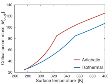
The red line of Fig.1shows the calculated relationship between the surface temperature and critical ocean mass be-yond which HP ice exists (see section2.5for the numerical procedure), which is abbreviated to COM-HP hereafter. It turns out that HP ice exists for an Earth-like planet with an ocean of more than ∼20 to ∼100 Moc,⊕, depending on
sur-face temperature. To see the sensitivity to the thermal struc-ture of the ocean, we also show the result for an isothermal ocean. The difference in COM-HP between the isothermal and adiabatic cases is ∼ 1–30Moc,⊕for Ts= 280–400 K. Even
for the two extreme cases, the difference is small enough not to change our conclusions.
2.2 Seafloor environment model
Near a mid-ocean ridge, heat flow from below is so high that the HP ice would be incapable of transporting the heat by thermal conduction nor convection and consequently be-come molten. If liquid water exists together with ice, the
20 40 60 80 100 120 140 260 280 300 320 340 360 380 400 Adiabatic Isothermal C ri ti ca l o ce a n ma ss [M OC, ] Surface temperature [K]
Figure 1. The critical ocean mass (COM-HP) in the unit of the Earth’s ocean mass (Moc,⊕), beyond which high-pressure (HP) ice
appears deep in the ocean is shown as a function of surface tem-perature (red line). Note that the result for an isothermal liquid ocean is also shown (blue line) to confirm that our calculation reproduces the result ofKitzmann et al.(2015) well.
heat can be transported efficiently by a sorbet flow, as de-scribed in Introduction. The HP ice far from a mid-ocean ridge remains solid because of low heat flow. Hence, there is a critical distance beyond which or a critical heat flow, qcr,
below which the HP ice remains solid.
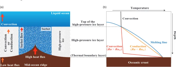
A schematic illustration of our seafloor environment model is shown in Fig.2. Here we assume that (1) the heat transport is steady and vertically one dimensional, (2) the composition and phase of H2O are vertically homogeneous
in the HP ice region, and (3) the sorbet flow dominates the heat transport in the solid-liquid coexistence region (called the sorbet region, hereafter), whereas solid-state convection or conduction occurs in the HP ice region. These assump-tions are consistent with results of previous hydrodynamical simulations (Choblet et al. 2017;Kalousov´a et al. 2018). We discuss their validity and impact on our conclusion in
sec-tion5.3.1.
2.2.1 Critical heat flow
First, we determine the critical distance or critical heat flow. Namely, according to its definition, we find the point at which convection nor conduction can hardly transport the heat inside the HP ice region. Figure2b shows qualitative temperature profiles in the HP ice: At the critical distance, since the ice-liquid mixture on the oceanic crust is in phase equilibrium, the temperature is equal to the melting tem-perature. Also, the temperature at the top of the HP layer is the melting one, by definition.
To determine the thermal structure of the HP ice region, we adopt a similar approach with that used by Fu et al.
(2010) who investigated the structure of the icy mantle of an ocean planet with a frozen surface, although they ignored horizontal variation in heat flux. UnlikeFu et al.(2010), we take into account the case where the HP ice layer is wholly conductive, ignore the upper thermal boundary layer, and
S or b et fl ow Convection Sorbet Mid-ocean ridge High heat flux Low heat flux
Liquid ocean C on ve c ti on or C on d u c ti on H igh -p r e ss u r e ice Top of the high-pressure ice layer
Conduction
(Ra < Racr)
Convection
(Ra > Racr)
Melting line
(Thermal boundary layer)
Temperature D e p th Oceanic crust (a) (b)
High-pressure ice layer
Convection
Figure 2. Seafloor environment model—(a) schematic illustration of the seafloor environment and (b) qualitative temperature profiles in the infinitesimally thin layer on the side of the high-pressure ice at the boundary between the ”sorbet” and ”high-pressure ice” regions. In panel (a), arrows represent the direction and dominant mechanisms of heat transport. In the sorbet region, ice and liquid coexist and thus the temperature is fixed at the melting point of H2O. In panel (b), Ra and Racrrepresent the Rayleigh number and the critical
Rayleigh number, respectively. The red and orange solid lines represent thermal structure when the high-pressure ice layer is convective and conductive, respectively. The blue and black solid lines represent the melting line of H2Oand adiabatic thermal structure of the
liquid ocean, respectively.
consider the different boundary condition for the bottom of the HP layer. The details are described below.
The mechanism of heat transport depends on the Rayleigh number, Ra, which is defined as
(Turcotte & Schubert 2002)
Ra= gαρD
3∆T HP
κη , (4)
where D is the thickness of the HP ice layer, κ is the co-efficient of thermal diffusivity, η is the viscosity, ∆THP=
TBBmel− TTBmel and TTBmel and TBBmel are the melting point
tem-peratures for the pressures at the top and bottom of the HP ice layer, respectively. For the melting point temperature Tmel, we use the formula fromDunaeva et al.(2010),
Tmel= a1+ a2P+ a3ln P+ a4P−1+ a5
√
P, (5) where P is the pressure in bar and the values of coefficients are summarized in Table1. We assume that the phase tran-sition from ice VI to VII occurs at the triple point of liq-uid/ice VI/ice VII, the pressure of which is 22160 bars. The thermal diffusivity is defined by κ = k/ρCP, where k is the
thermal conductivity. For CP of ice VI and VII, we use the
expression derived by Fei et al. (1993). For k, we adopt a constant value of 3.8 Wm−1K−1, which is its typical value
for ice VII under 2.5 GPa and 300 K (Chen et al. 2011), for simplicity. For η of ice VII, which is poorly constrained, we adopt a dislocation model for the viscosity of phase VI, which is the highest phase of the HP ice measured so far
(Durham et al. 1997) : η(Pη, Tη) = Bζ−3.5exp !(E∗+ P ηV∗) RTη " , (6) where B (= 6.7 × 10¹⁹ Pa4.5 s) is a constant, ζ (= 2.0 ×
106 Pa) is a characteristic shear stress (Fu et al. 2010), R is the ideal gas constant, E∗ (= 110 kJ mol−1) and V∗
(= 1.1 × 10⁻⁵ m3 mol−1) are the activation energy and
vol-ume (Durham et al. 1997), respectively, and Tη and Pη are
Table 1.Coefficients for ice melting curve given by Eq. (5) from Dunaeva et al.(2010)
Ice phase a1 a2 a3 a4 a5
Ice VI 4.2804 -0.0013 21.8756 1.0018 1.0785 Ice VII -1355.42 0.0018 167.0609 -0.6633 0
the temperature and pressure at deformation, respectively. Because the viscosity contrast in the HP ice layer is rela-tively small, the small viscosity contrast prescription can be used (Fu et al. 2010). For Pη and, Tη, we use the averaged
values for the HP ice layer (Dumoulin et al. 1999). In this study, we assume the value of the critical Rayleigh number, Racr, is 2000.
When Ra < Racr, conduction dominates heat transport
and, thus, qcr is given as
qcr= k
∆THP
D . (7)
When Ra > Racr, since convection occurs, we assume
the adiabatic temperature gradient (i.e., Eq.[3]). Near phys-ical boundaries, however, since convective motion is pre-vented, thermal boundary layers are formed, where conduc-tion transports heat. In this study, we consider the presence of a boundary layer only on the bottom of the HP ice layer (BBL), where the temperature gradient is given by
dT dr = −
q
k (8)
and q is the heat flux. Integrating Eq. (3) inwards from the top of the HP ice layer and Eq. (8) outwards from the surface of the oceanic crust, we determine the BBL’s thickness, δ , and the temperature difference in the BBL, ∆TBBL at the
crossover point for a given q (see Fig.2b).
convection, Ra = Racr in the BBL, namely, Racr = gαρδ3∆T BBL/κηBBL, which comes to be δ =# κηBBLRacr gαρ∆TBBL $1/3 , (9)
where ηBBL is the viscosity of the HP ice in the BBL and
calculated with the intermediate values of temperature and pressure between the top and bottom of the BBL. If the set of δ and ∆TBBL for a given q satisfies Eq. (9), the value of q
corresponds to qcr, which is also written as
qcr= k ∆TBBL δ = kκRacr gαρ · ηBBL δ4 . (10)
Note thatFu et al.(2010) considered a boundary layer under the top of the HP ice layer in addition to BBL. We discuss the difference in temperature structure in the HP ice layer between this study andFu et al.(2010) and its impacts on our conclusion in section5.3.1.
2.2.2 Effective weathering area
Same as in the Earth, the oceanic crust is assumed to form via eruption of hot mantle rock only at the mid-ocean ridge. As it moves away from the mid-ocean ridge toward the trench, the oceanic crust is cooled by seawater. Here we define a non-dimensional effective weathering area, foc, as
the area of the sorbet region (i.e., q > qcr) relative to the
whole area of oceanic crust. A constant rate of oceanic crust production being assumed, foc is equivalent to the ratio of
the period during which q ≥ qcrto the residence time of the
oceanic crust, τ.
To calculate foc, we model the cooling of the oceanic
crust, adopting the semi-infinite half-space cooling model
(Turcotte & Schubert 2002): This model assumes that the
crust cools only by vertical heat conduction. The heat flux from the oceanic crust is given by (Turcotte & Schubert
2002)
q(t) =krock√(Tπκsol− Tfloor)
rockt ≡
A √
t, (11) where t is time, krock (= 3.3 W m−1 K−1) and κrock (=
1.0 × 10⁻⁶ m2 s−1) are the thermal conductivity and
ther-mal diffusivity of the oceanic crust, respectively, Tfloor is
the seafloor temperature, and Tsolis the potential
tempera-ture of the mantle, for which we assume the peridotite dry solidus at the seafloor pressure, which was parameterized
byHirschmann et al.(2009). This assumption is made just
for simplicity. The influence of the assumption on planetary climate is discussed in section5.2.
From Eq. (11), the length of time required for q to decrease to qcr, which is denoted by tcr, is given by tcr=
A2/q2
cr. Also, if the mean mantle heat flow, ¯q, is defined as
¯
q ≡ τ−1%τ
0qdt, the residence time τ is given as a function of
¯
qas τ = 4A2/ ¯q2. Thus, the effective weathering area is given
as foc≡ tcr τ = 1 4 # ¯ q qcr $2 . (12) In some cases, calculated tcr happens to be larger than τ,
which means the oceanic crust is fully covered with the solid-liquid mixture (i.e., the sorbet). In such cases, we set foc= 1.
From Eq. (12), it turns out that when qcr> ¯q/2, solid HP
ice appears near the trench. In the next section, we use foc
in the carbon cycle model.
In this study, the mean mantle heat flow ¯q is a free parameter. As the fiducial value, we use ¯q = 80 mW m−2,
which is the value for the present Earth. Note that qcr is
independent of ¯q, according to Eq. (12).
2.3 Carbon cycle model
In order to investigate planetary climate, we develop a carbon cycle model by modifying the Earth’s carbon cy-cle model of Tajika & Matsui (1992). Since we focus on continent-free terrestrial planets, we add the effect of seafloor weathering and neglect the continental reservoir of carbon and the effect of continental weathering. In addi-tion, we consider the presence of the HP ice and pressure-dependent degassing. Same asTajika & Matsui(1992) and
Sleep & Zahnle(2001), we perform box-model calculations
of carbon circulation among reservoirs and find the equilib-rium states.
2.3.1 Carbon reservoirs
We consider four reservoirs, which include the atmosphere, ocean (liquid water plus HP ice), oceanic crust (basalt), and mantle. Between the atmosphere and ocean, however, the carbon partition is assumed to be always in equilib-rium, which is described in detail in Appendix B. The equilibrium value of the CO2 partial pressure PCO2
de-pends on the number of cations dissolved in the ocean (e.g.,Zeebe & Wolf-Gladrow 2001), for which we assume the present Earth’s value, although the supply of cations via con-tinental weathering never occurs in ocean planets. We have confirmed that overall results are insensitive to the number of dissolved cations (even in the case with no cations in the ocean). This is because the ocean reservoir is much small relative to the whole planetary carbon reservoir.
Carbon dissolved in the ocean is carried to the seafloor in the form of CO2ice, into which aqueous CO2is converted
in the sorbet region (Bollengier et al. 2013). We assume that the carbon circulation in the sorbet region occurs quickly enough that it never affects the mass balance and also plan-etary climate. Detailed discussion of the CO2 circulation is
given in section5.3.1.
The origin of volatiles in terrestrial planets has been highly debated so far, even for the Earth (e.g.,O’Brien et al. 2018). Since possible candidates such as carbonaceous chon-drites and comets include both carbon compounds and wa-ter, we assume that the total mole number of carbon con-tained in the whole planet, Ctotal, is proportional to ocean
mass, namely
Ctotal= γ noc,⊕
Moc
Moc,⊕
, (13) where γ is the CO2/H2Omolar ratio in the source of volatiles
of the planet, noc,⊕(= 7.6 ×10²²mol) is the molar quantity of
H2Oin the Earth ocean mass, and Moc,⊕(= 1.37 × 10²¹ kg)
is the Earth’s ocean mass. Using the data and estima-tion published, we can estimate γ is to be 0.22 for car-bonaceous chondrites (Jarosewich 1990), 0.71 for comae of
comets (Marty et al. 2016), and 0.19 for Earth composi-tion (Tajika & Matsui 1992). We use the Earth-like value (γ = 0.19) as the fiducial value. Dependence of planetary cli-mate on γ is discussed in sections4.
2.3.2 Carbon budget
The mass balance among those reservoirs is expressed as d(Catm+Coc) dt = FD+ FM− FSW, (14) dCbs dt = FSW− FR− FM, (15) dCman dt = FR− FD, (16) Ctotal = Catm+Coc+Cbs+Cman, (17)
where Catm, Coc, Cbs, and Cman are the mole numbers of
car-bon contained in the atmosphere, ocean, oceanic basalt, and mantle, respectively, and FSW, FD, FR, FM are the
car-bon fluxes due to seafloor weathering, degassing from the mid-ocean ridge, regassing via subduction into mantle and metamorphism that leads to degassing from volcanic arc, re-spectively. Those equations are solved for a given value of Ctotal.
We adopt the degassing, regassing, and metamorphism models fromTajika & Matsui(1992), where each flux is ex-pressed as FD = KDASCman, (18) FR = β τCbs, (19) FM = 1 − β τ Cbs. (20) Here KD is the molar fraction of carbon degassing as CO2
from the erupting magma per unit area. We take into ac-count the dependence of KDon seafloor pressure (i.e., ocean
mass), the detail of which is described in AppendixC. β is the regassing ratio defined as the molar fraction of carbonate regassed into the mantle in the total subducting carbonate. We adopt the present Earth’s value of β (= 0.4) estimated
byTajika & Matsui(1992). ASis the seafloor spreading rate,
which is simply given by AS=
A0
τ , (21) where A0 is the whole area of the seafloor. We assume
that A0 is the present Earth’s value (= 3.1 × 10¹⁴ m2) from
McGovern & Schubert(1989) and calculate τ from the
rela-tion τ = 4A2/ ¯q2 for a given ¯q.
The seafloor weathering rate FSW depends on seafloor
temperature Tfloor as (Brady & G´ıslason 1997)
FSW= FSW∗ focexp ! Ea R # 1 T0− 1 Tfloor $" , (22) where F∗
SW is the present Earth’s seafloor weathering rate,
foc is the effective weathering area given by Eq. (12), Ea
is the activation energy, and T0 (= 289 K) is the reference
seafloor temperature that corresponds to the surface temper-ature obtained by the atmospheric model with the present Earth’s condition. F∗
SW estimated from deep-sea cores is
1.5–2.9 × 10¹² mol yr−1(Alt & Teagle 1999;Staudigel et al.
1989; Gillis & Coogan 2011). In this study, we use F∗
SW =
2.0 × 10¹² mol yr−1.
The activation energy Ea is uncertain and its
re-ported value ranges between 30 and 92 kJ mol−1.
Brady & G´ıslason (1997) firstly determined Ea
experimen-tally to be 41 kJ mol−1. Recent inversion methods
us-ing geological evidence support a relatively high value of Ea: Precisely, strontium and oxygen isotopes in carbonates
indicated Ea= 92 ± 7 kJ mol−1 (Coogan & Dosso 2015).
Also, several proxies reflecting the surface and seafloor tem-peratures, atmospheric CO2, and oceanic pH showed Ea=
75+22−21kJ mol−1(Krissansen-Totton & Catling 2017). Those
values are also consistent with estimates from laboratory experiments for the dominant minerals in the oceanic crust
(Brantley & Olsen 2013). In contrast, an experimental study
of basalt dissolution in the moderate pH range reported the relatively small Eaof 30 kJ mol−1 (Gudbrandsson et al. 2011). In this study, we use Ea= 41 kJ mol−1 as the
fidu-cial value according to previous studies (e.g., Foley 2015) and vary it over the range between 30 and 92 kJ mol−1.
We ignore the pH dependence of seafloor weathering since it is known to be small in the pH range between 4 and 10
(Gudbrandsson et al. 2011).
The seafloor temperature also depends on the surface temperature, Ts, because we assume that the temperature
structure of the ocean is adiabatic (see also §2.1). We cal-culate Ts as a function of PCO2, as described in detail in
section 2.4. On the area of the seafloor beneath the sor-bet region, Tflooris equal to the melting temperature at the
seafloor pressure.
2.4 Atmospheric model
In this study, we use the open-source code for 1-D radiative-convective climate models, Atmos1, developed by Kasting
and his collaborators (Kasting et al. 1993;Kopparapu et al.
2013; Ramirez et al. 2014). This code calculates radiative
fluxes in vertically spacing layers of the atmosphere, us-ing the two-stream approximation with the coefficients for radiative absorption and scattering by gaseous molecules updated by Kopparapu et al. (2013). We assume a 1-bar N2 atmosphere with various partial pressures of CO2. The
distribution of the relative humidity of water vapor is treated according to the empirical Manabe-Wetherald model which assumes the surface relative humidity of 0.8, based on the present Earth’s atmosphere (Manabe & Wetherald
1967; Pavlov et al. 2000). According to Kopparapu et al.
(2013), we use the surface albedo of 0.32, which implic-itly includes the effects of present-day Earth water clouds. We use the present insolation flux at the Earth’s orbit S⊙ (=1360 W m−2) and the present Sun’s spectrum as
the fiducial value and spectrum model, respectively. The other model settings are the same as those adopted in
Ramirez et al. (2014). Then, we calculate equilibrium
val-ues of Ts as a function of PCO2 for given stellar insolation,
using a time-stepping approach with moist convective ad-justment (Pavlov et al. 2000). We have confirmed that our calculated Tsis almost the same with sufficient accuracy as
that from Ramirez et al.(2014). We discuss the uncertain-ties and impacts of stellar insolation, surface albedo, and relative humidity in sections4.2,5.3.2, and5.4.
2.5 Numerical procedure
In summary, for given values of ocean mass Moc and mean
mantle heat flow ¯q, we determine the climate of the ocean planet by the following procedure.
(i) For trial values of surface temperature Ts and surface
pressure Ps, we integrate Eqs. (1)–(3) inward from the
sur-face to determine temperature as a function of pressure in the ocean (see § 2.1). We find a level where the adiabat crosses the melting temperature of ice. The layer between the crossover level and the oceanic crust surface consists of HP ice. Then, the seafloor pressure Pfloorand the thickness of
the HP ice layer D are determined. If the adiabat reaches the oceanic crust surface before crossing the ice melting curve, the planet has no ice in the deep ocean. The numerical inte-gration is performed with a 4th-order Runge-Kutta method. The size of the interval is chosen so that the pressure at the crossover point is determined with < 0.1 % accuracy.
(ii) When the HP ice is present, from the seafloor environ-ment model, we determines the critical heat flow qcr (or the
area of the sorbet region) from Eq. (7) or (10), depending on Ra (§2.2). Then, we obtain the effective weathering area focby substituting qcrand ¯q in Eq. (12). Also, we obtain the
seafloor temperature Tfloorin the sorbet region by
substitut-ing Pfloorin Eq. (5).
(iii) In the carbon cycle model (§2.3), using Tfloor and foc
obtained above, we perform a time integration of Eqs. (14)– (16) and determine the carbon partition among the atmo-sphere, ocean, oceanic crust, and mantle. Then, from the calculated PCO2, we obtain a new value of Ts (and thereby
Ps) from the atmospheric model (§2.4). If the new value of
Ts differs by > 0.01 K from the trial value of Ts, we return
to Step (i) and repeat the above procedures with the new Ts. The time integration is performed with a Euler method
and the interval size is chosen so that the time difference in the molar number of carbons is smaller than 0.1 % for all the reservoirs.
(iv) Once all the time derivatives in Eqs. (14)–(16) become zero, we judge the solution as an equilibrium state. If the surface temperature drops below 273 K, we also stop the time integration and regard the solution as a snowball state. We start time-stepping calculations at arbitrarily high PCO2 (i.e., in a warm condition) for finding equilibrium
so-lutions. We have confirmed that the results are insensitive to choice of the initial condition, provided a sufficiently high CO2pressure (PCO2> 10 bars) is adopted. (The carbon cycle
and climate stability in the snowball state are discussed in section 5.3.3.) In most of our simulations, response against perturbations for the carbon budget in the atmosphere-ocean system is mainly controlled by regassing, the timescale of which is ∼ τ/β = 250 Myr for ¯q = 80 mW m−2. Thus, an
equilibrium state is achieved on a timescale of the order of Gyr, which is also consistent with results shown in Foley
(2015).
The parameters and constants with their values adopted
in this study are summarized in Tables 2 and 3, respec-tively. The upper limit for ocean mass Mocthat we consider
is 200 Moc,⊕. The reasoning is as follows: We suppose that
plate tectonics is working on the planet. Although still not fully understood, an increase in water has negative effects on plate tectonics. In particular, it leads to reducing crustal pro-duction and degassing, since the solidus temperature of the mantle material increases with pressure (Kite et al. 2009;
Noack et al. 2016). According toNoack et al.(2016), crustal
production completely ceases for an Earth-mass planet with the ocean layer thicker than approximately 400 km, if plate tectonics operates. The ocean mass of 200 Moc,⊕ that we
adopt here corresponds to the ocean layer of ∼350 km for Ts= 300 K. We do not consider ocean planets with more
massive oceans because such planets are expected to have no geochemical cycle. For planetary climates with no geo-chemical cycle, seeKitzmann et al.(2015) andKite & Ford
(2018).
Note that we assume a spherically symmetric struc-ture in the internal strucstruc-ture modeling, while we consider the presence of the sorbet and HP ice regions in the deep ocean in the seafloor environment modeling. Such self-contradiction, however, has little influence on our whole modeling. This is because only the thermal structure above the HP ice layer is of interest in this study and the equa-tions of state of water, rock, and iron are rather insensitive to temperature.
3 MELTING OF THE HP ICE
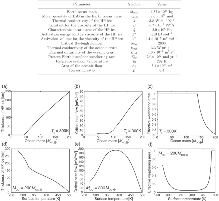
We first investigate the behavior of the HP ice with a focus on the effective weathering area, which is a controlling factor for seafloor weathering. Here we do not use the carbon cycle model, but, instead, perform calculations for fixed values of the surface temperature Ts. Figure3shows the calculated
thickness of the HP ice layer D (left column), the critical heat flow qcr (middle column) and effective weathering area foc
(right column) as a function of ocean mass Mocfor Ts= 300 K
(top) and as a function of Tsfor Moc= 200Moc,⊕(bottom). In
those calculations, the mean mantle heat flow ¯q is assumed to be 80 mW m−2.
3.1 Dependence on Ocean Mass
The overall dependence on ocean mass is as follows. As shown in Fig. 3a, the HP ice is present, if Moc" 45Moc,⊕.
Its thickness increases almost linearly with ocean mass and reaches 247 km at Moc = 200Moc,⊕. In Fig.3b, the critical
heat flow is found to be zero for Moc! 45Moc,⊕, because of
no HP ice, and then increase with ocean mass, up to about 80mW m−2(≃ ¯q) at Moc= 200Moc
,⊕. In Fig.3c, the effective
weathering area is found to be unity until Moc≃ 139Moc,⊕
and rapidly decrease to about 0.2 at Moc= 200Moc,⊕.
A jump in qcr is found at Moc≃ 74Moc,⊕ in Fig. 3b.
At that point, the heat transport mechanism in the HP ice above the critical point (i.e., q = qcr) changes from
conduc-tion to convecconduc-tion. For Moc! 74Moc,⊕(D ≃ 55 km), the HP
ice layer is thin enough and, therefore, the temperature dif-ference ∆THP(= TBBmel− TTBmel) is small enough for conduction
to transport the heat flux from the oceanic crust. However, as shown in Fig3c, qcr≃ 10 mW m−2< ¯q/2 at Moc! 74Moc,⊕,
Table 2.Variables and their values.
Parameter Symbol Value
Ocean mass Moc 1–200 Moc,⊕
Mean mantle heat flow q¯ 40, 60, 80, 100, 120 mW m−2
Activation energy of seafloor weathering Ea 30, 41, 92 kJ mol−1
CO2/H2Omolar ratio γ 1.0 × 10⁻³–10
Table 3.Parameters and their values.
Parameter Symbol Value
Earth ocean mass Moc,⊕ 1.37 × 10²¹ kg
Molar quantity of H2Oin the Earth ocean mass noc,⊕ 7.6 × 10²²mol
Thermal conductivity of the HP ice k 3.8 W m−1K−1
Constant for the viscosity of the HP ice B 6.7 × 10¹⁹Pa4.5s
Characteristic shear stress of the HP ice ζ 2.0 × 10⁶ Pa
Activation energy for the viscosity of the HP ice E∗ 110 kJ mol−1
Activation volume for the viscosity of the HP ice V∗ 1.1 × 10⁻⁵m3mol−1
Critical Rayleigh number Racr 2000
Thermal conductivity of the oceanic crust krock 3.3 W m2s−1
Thermal diffusivity of the oceanic crust κrock 1.0 × 10⁻⁶m2s−1
Present Earth’s seafloor weathering rate F∗
SW 2.0 × 10
12mol yr−1
Reference seafloor temperature T0 289 K
Area of the oceanic floor A0 3.1 × 10¹⁴m2
Regassing ratio β 0.4
(a)
(b)
(c)
(d)
(f)
0 50 100 150 200 250 0 50 100 150 200Ocean mass [MOC, ]
T h ickn e ss o f H P ice [ km] T s = 300K 0 10 20 30 40 50 60 70 80 90 0 50 100 150 200 C ri ti ca l h e a t fl o w [ mW /m 2] 0.2 0.3 0.4 0.5 0.6 0.7 0.8 0.9 1 0 50 100 150 200 Ef fe ct ive w e a th e ri n g a re a 0 50 100 150 200 250 300 250 300 350 400 450 500 T h ickn e ss o f H P ice [ km] Surface temperature[K] 0 20 40 60 80 100 120 140 160 180 200 250 300 350 400 450 500 C ri ti ca l h e a t fl o w [ mW /m 2] Surface temperature[K] 0 0.2 0.4 0.6 0.8 1 250 300 350 400 450 500 Ef fe ct ive w e a th e ri n g a re a Surface temperature[K]
(e)
T s = 300K Ts = 300KOcean mass [MOC, ] Ocean mass [MOC, ]
M OC = 200MOC, M OC = 200MOC, M OC = 200MOC,
Figure 3.Formation of high-pressure (HP) ice and its impacts on the seafloor condition. Thickness of the HP ice layer (panels a and d), critical heat flow (panels b and e), and effective weathering area (panels c and f ) are shown as a function of ocean mass Mocfor surface
temperature Ts= 300 K (top) and as a function of Ts for Moc= 200Moc,⊕ (bottom). Moc,⊕represents the present Earth’s ocean mass. Note
0 20 40 60 80 100 120 140 160 180 200 100 110 120 130 140 150 160 170 180 190 200 0 0.2 0.4 0.6 0.8 1
Ocean mass [MOC, ]
Critical heat flow Effective weathering area
C ri ti ca l h e a t fl o w [ mW /m 2] Ef fe ct ive w e a th e ri n g a re a
Figure 4. The maximum of critical heat flow (red solid line) and the minimum of effective weathering area (blue solid line) found in the surface temperature range considered in this study are shown as a function of ocean mass. In these calculations, we have assumed the mean mantle heat flux ¯q = 80 mW m−2.
meaning that the HP ice is entirely molten (i.e., foc= 1),
that is, the seafloor is covered entirely with the sorbet for Moc! 74Moc,⊕(see the text just below Eq. [12]). Note that
discontinuities in qcr or dqcr/dMoc found at Moc≃ 86 and
103Moc,⊕ come from those in the melting curve of H2Oat
the phase boundaries of ice VI/VII.
The critical heat flow exceeds ¯q/2 at Moc≃ 139 Moc,⊕
(D ≃ 160 km), until which the effective weathering area is unity, and then increases further with ocean mass. Such an increase in qcr occurs because the Rayleigh number in the
HP ice layer increases. Thus, the effective weathering area decreases with ocean mass, but never becomes zero until Moc= 200Moc,⊕. This means that water-rock reactions
be-tween water and rock including the seafloor weathering are possible, despite the presence of the thick HP ice, because the sorbet region also exists near the mid-ocean ridge.
3.2 Dependence on Surface Temperature
The three lower panels of Fig. 3 show the dependence on the surface temperature for Moc = 200Moc,⊕. The HP ice
thickness decreases, as the surface temperature increases, as shown in Fig.3d. At Ts≃ 320 K, the curve is a bit inflected.
This is due to the phase change of HP ice from ice VI to ice VII.
In Figs. 3e and3f, we find a maximum of the critical heat flow and a minimum of the effective weathering area, respectively, at Ts≃ 390 K. As indicated in Eq. (10), qcr
depends on ηBBLand δ , both of which decrease with Ts. For
Ts!390 K, δ4decreases more rapidly than ηBBL and, thus,
qcr increases with Ts. In contrast, for Ts" 390 K, the latter
dominates over the former, so that qcr decreases. At Ts≃
390 K, ∂ (ηBBL/δ4)/∂ Ts= 0. The behavior of the effective
weathering area can be readily understood from Eq. (12), namely, foc∝ q−2cr . The minimum is foc≃ 0.04.
In Fig. 4, we show the maximum of critical heat flow qcr,maxand minimum of effective weathering area foc,minas a
function of ocean mass for ¯q = 80 mW m−2. Here we show
only the results for the case of convective HP ice for Moc>
100Moc,⊕ because the critical heat flow due to conduction is
small. While qcr,maxis found to monotonically increase with
Moc, foc,minbegins to drop with Mocat Moc≃ 128Moc,⊕, which
is smaller than in the case of Ts= 300 K because of difference
in Ts. The blue line in Fig.4indicates that even the minimum
of focis unity for Moc! 128Moc,⊕, which means that the HP
ice is entirely molten and the seafloor is completely covered with the sorbet, regardless of surface temperature, in such an ocean mass range for the Earth-like mean mantle heat flow ( ¯q = 80 mW m−2). Also, foc,min> 0, meaning that seafloor
weathering works, even if Moc= 200Moc,⊕.
4 SEAFLOOR WEATHERING ENHANCED BY THE HP ICE
4.1 Consequence of carbon cycle
Here we examine the planetary climate based on the carbon cycle including the effective weathering area obtained above. The calculation results for ¯q = 80 mW m−2, γ = 0.19, and
S= S⊙ and 0.9S⊙ are shown in Fig.5, where (a) the surface and seafloor temperatures, (b) the seafloor weathering flux and effective weathering area, and (c) the partial pressure of atmospheric CO2are plotted as functions of the ocean mass.
In Fig.5a, two obviously different states are found: One is the state with Ts> 273 K, where the carbon cycle is in a
steady state, the other, as indicated by a shaded area, is the state with Ts= 273 K, where the carbon cycle calculation is
artificially stopped at Ts= 273 K because the surface ice is
expected to form (see also §2.5). The former is called the equilibrium state and the latter is called the snowball state in this study. In this case, the HP ice begins to form at Moc
= 86Moc,⊕. It turns out that the formation of the HP ice has
a drastic effect on the carbon cycle and determines which state is achieved.
In the case of no HP ice (i.e., Moc< 86Moc,⊕), both the
surface temperature and CO2 partial pressure increase with
ocean mass. An equilibrium state is achieved for a given ocean mass via a negative feedback loop such that an in-crease in PCO2 raises the surface temperature, which leads
to a rise in seafloor temperature, which enhances seafloor weathering flux, which finally reduces the atmospheric CO2.
The larger the ocean mass, the larger the total carbon in-ventory Ctotalis (see Eq. [13]). Since an increase in Ctotal
en-hances the degassing flux of CO2(see Eq. [18]), the surface
temperature consequently raises with ocean mass. This is, in other words, because the enhancement of the degassing flux dominates over the increase in seafloor temperature in the case of γ = 0.19. While the outcome depends on γ, we have confirmed that this trend is the same also in the case of one-tenth of the Earth-like value γ (= 0.019) and comet-like γ (= 0.71) higher than the Earth’s: The equilibrium values of Ts and PCO2 for Moc< 86Moc,⊕ are increased up to 326 K
and 2.4 × 10⁻¹ bars for γ = 0.19 and S
⊙, respectively (see
Figs.5aand5c).
In contrast, when the HP ice is present (Moc≥ 86Moc,⊕),
the negative feedback never works and, consequently, the snowball state is attained. This is because the seafloor tem-perature on the area under the sorbet region, where seafloor weathering works, is fixed at the melting temperature of ice and, thus, insensitive to the surface temperature. Although
270 280 290 300 310 320 330 0 50 100 150 200 250 300 350 400 450 500 550 (a) Su rf a ce t e mp e ra tu re [ K]
Surface temperature Seafloor temperature
Se a flo o r te mp e ra tu re [K]
Ocean mass [MOC, ]
12 13 14 15 16 0 50 100 150 200 0.65 0.7 0.75 0.8 0.85 0.9 0.95 1 (b) Se a fl o o r w e a th e ri n g f lu x [l o g (mo l/ ye a r)] Ef fe ct ive w e a th e ri n g a re a
Seafloor weathering flux Effective weathering area
0 50 100 150 200 (c) Pa rt ia l p re ssu re o f C O2 [l o g (b a r)]
Ocean mass [MOC, ]
1.0S 0.9S -6 -5 -4 -3 -2 -1 0
Ocean mass [MOC, ]
Figure 5.Surface and seafloor conditions obtained from the carbon cycle model: (a) Surface temperature (red sold line) and seafloor temperature (red dashed line), (b) seafloor weathering flux (blue solid line) and effective weathering area (blue dashed line), and (c) partial pressure of CO2 are shown as a function of ocean mass in the unit of the Earth’s ocean mass Moc,⊕. Shaded is the range for
the snowball state. In this calculation, the mean mantle heat flow is assumed to be 80 mW m−2. The symbol S
⊙ represents the solar
insolation received by the present Earth.
the reduction in effective weathering area reduces seafloor weathering rate (see Fig.5b), it is found to have little impact on surface temperature because the seafloor weathering flux is significantly higher than the degassing flux.
4.2 Dependence on stellar insolation
We examine the dependence of planetary climate on stellar insolation. Since the runaway greenhouse limit, which con-trols the inner edge of the habitable zone, is only slightly higher than S⊙ (e.g., 1.06S⊙ Kopparapu et al. 2013), we show only the results for smaller stellar insolation of 0.9S⊙ than the fiducial value of 1.0S⊙. As shown in Fig. 5c, stel-lar insolation affects CO2 partial pressure both in the
equi-librium and snowball states: the smaller the stellar insola-tion, the higher the CO2 pressure is, as a whole: PCO2 for
S= 0.9S⊙ is higher by a factor of ∼ 3 and by two orders of magnitude than that for S = 1.0S⊙in the equilibrium and snowball states, respectively. The other quantities are almost unaffected by stellar insolation. This is because the increase in CO2 pressure compensates for the decline in stellar
in-solation so as not to change the surface temperature which controls weathering behavior and COM-HP in our climate model. Thus, variation in stellar insolation has little impact on planetary climate, provided the planet is located in the habitable zone.
4.3 Dependence on mean mantle heat flow
Next, we examine what impact the mean mantle heat flow ¯
qhas on the surface and seafloor conditions. Figure6shows (a) the surface temperature, (b) effective weathering area, and (c) seafloor weathering flux for five different choices of
¯
q. The variation in mean mantle heat flow turns out to yield no change on the overall behavior, but quantitative modifi-cations to the ocean mass dependence.
First, as seen in Fig. 6a, when no HP ice is present, the larger the mean mantle heat flow, the higher the surface temperature is for a given ocean mass. The variation in ¯q leads to a large difference in the surface temperature (up to 40 K). Also, the surface condition lapses into the snow-ball state at larger ocean mass for a larger ¯q. That is be-cause as ¯q increases, the seafloor spreading rate ASincreases
(see Eq. [21]) and, thus, the degassing flux increases (see Eq. [18]), leading to higher surface temperature and larger critical ocean mass for forming the HP ice (COM-HP, see also Fig.1). In Fig.6c, the seafloor weathering flux is also found to increase by approximately an order of magnitude in response to the rise in the degassing flux.
As shown in Fig. 6b, the effective weathering area foc starts to decrease from unity at larger ocean mass for
larger mean mantle heat flow and is always unity until Moc= 200Moc,⊕ for ¯q ≥ 100 mW m−2. While the seafloor
weathering flux changes with ¯q (i.e., foc) in the case with
HP ice, the reduction in focturns out to have only a small
effect on the surface temperature, because of significantly high seafloor weathering rate for any value of ¯q (see Fig.6c).
4.4 Dependence on CO2/H2O ratio and seafloor
weathering activation energy
As described in section2.3, the carbon cycle depends on the total carbon inventory and seafloor weathering rate. The for-mer may differ greatly from planet to planet, as suggested, for example, by a difference in the CO2/H2Omolar ratio γ
(Eq. [13]) between comets and the Earth. Also, the seafloor weathering rate is in general uncertain, mainly because the activation energy Ea(Eq. [22]) is poorly determined
observa-tionally. Here we investigate the sensitivities of the planetary climate to γ and Ea with focus on the critical ocean mass,
beyond which the planetary climate is in the snowball state (hereafter, abbreviated to COM-SB and denoted by Moccr(sb)).
In Fig. 7, we plot the relationships between Moccr(sb)
and total degassing flux, FD+ FM, for various values of γ
between 7.4 × 10⁻³ and 2.1; both Moccr(sb) and FD+ FM are
obtained from the carbon cycle calculations. Here we as-sume ¯q = 80 mW m−2. Fig. 7ashows the fiducial case with
Ea= 41 kJ mol−1; Fig.7b shows cases with three different
values of Ea. For reference, in Fig. 7a, we show the
rela-tionships between FD+ FMand not Moccr(sb)but Mocfor three
different values of γ by dashed lines (the result for γ = 0.19 is also shown in Fig.5b). In Fig.7a, we can see that the to-tal degassing flux increase almost linearly with γ for a given ocean mass. For γ < 7.4 × 10⁻³, the COM-SB is absent
270 280 290 300 310 320 330 340 350 0 50 100 150 200
(a)
40 mW/m2 60 mW/m2 80 mW/m2 100 mW/m2 120 mW/m2 Su rf a ce t e mp e ra tu re [ K]Ocean mass [MOC, ]
0.1 0.2 0.3 0.4 0.5 0.6 0.7 0.8 0.9 1 0 50 100 150 200
(b)
Ef fe ct ive w e a th e ri n g a re a 40 mW/m2 60 mW/m2 80 mW/m2 100 mW/m2Ocean mass [MOC, ]
11 12 13 14 15 16 0 50 100 150 200 Ocean mass [MOC, ]
(c)
Se a fl o o r w e a th e ri n g f lu x [ lo g (mo l/ ye a r)] 40 mW/m2 60 mW/m2 80 mW/m2 100 mW/m2 120 mW/m2Figure 6.Surface and seafloor conditions obtained from the car-bon cycle model for five different values of the mean mantle heat flow. (a) Surface temperature, (b) effective weathering area and (c) seafloor weathering flux are shown as functions of ocean mass.
cause the snowball state is achieved in all the ocean mass range due to low degassing flux.
As shown in Fig. 7a, the total degassing flux has a peak at Moccr(sb)= 128Moc,⊕. For Moccr(sb)≤ 128Moc,⊕, the
COM-SB increases from 24 to 128 Moc,⊕ and the total degassing
flux, which is determined by FSW(Tfloor, foc) = FSW(Tfloormel, 1),
increases from 8.1 × 10¹¹ to 6.8 × 10¹⁴ mol yr−1 with
in-crease in γ from 7.4×10⁻³to 2.1. Despite order-of-magnitude
variation in FD+ FM, the COM-SB varies moderately by a
factor of ∼5 (see section 5.1 for an analytical interpreta-tion). On the other hand, for Moccr(sb)> 128Moc,⊕, the total
de-gassing flux is determined by the minimum weathering flux
with the HP ice, namely FSW(Tfloor, foc) = FSW(Tfloormel, foc,min)
(see Fig. 4for foc,min). Thus, the COM-SB increases from
128 to 200Moc,⊕ and the total degassing flux decreases from
6.8 × 10¹⁴ to 2.3 × 10¹⁴ mol yr−1 with decrease in γ from
2.1 to 5.2 × 10⁻¹. In this diagram, equilibrium climates (FSW
= FD+ FM) are achieved on the side above the solid line,
whereas the planetary surface condition lapses into snowball states (FSW> FD+ FM), because of the presence of the sorbet
region, on the side below the solid line. Note the curve of Mcr(sb)oc is a bit inflected at Moc= 85Moc,⊕because of a phase
change of the HP ice.
In Fig. 7b, we show the impact of Ea on Moccr(sb). The
curve for larger Eais found to be steeper. The three curves
cross each other at FD+ FM= 2.0 × 10¹² mol yr−1, where the
seafloor temperature Tfloor is equal to T0 (=289 K), so that
FSWis independent of Ea(see Eq. [22]). Above the crossover
point, the higher the activation energy, the smaller the COM-SB is; its dependence is opposite below the crossover point. Although being large relative to that on γ, the de-pendence of Moccr(sb)on Ea is at most linear. Thus, it would
be fair to say that Mcr(sb)oc is rather insensitive to Ea. We
further discuss the nature of the COM-SB analytically in section5.1.
5 DISCUSSION
5.1 Critical ocean mass for snowball state
One of the most important findings in this study is that there is a critical ocean mass, beyond which an ocean ter-restrial planet has an extremely cold climate (i.e., the snow-ball state). Furthermore, we have found that the COM-SB, Mcr(sb)oc , falls into a relatively narrow range between 20 and
100 Moc,⊕. Here we give an interpretation to the low
sensitiv-ity of Moccr(sb)to the planetary mass Mp, the total degassing
flux FD+ FM, and the activation energy of seafloor
weather-ing Ea, by deriving an approximate solution for Moccr(sb). This
could help us obtain an integrated view of planetary climate on ocean planets under our idealized seafloor environments. As demonstrated in section 4, the planetary climate lapses into the extremely cold one, when HP ice is formed on the seafloor. Then, the seafloor temperature Tflooris fixed at
the melting temperature Tmeland thus determined uniquely
by the seafloor pressure Pfloor. Since the ocean mass and
depth are negligibly small relative to the planetary mass and radius, respectively, under hydrostatic equilibrium, the seafloor pressure is given approximately by
Pfloor ≈ GMp 4πR4 p Moc= G ¯ρp 3Rp Moc, (23)
where Rp and ¯ρp are the planetary radius and mean
den-sity, respectively. For Moc = Moccr(sb), Pfloor corresponds to
the crossover pressure between the adiabat and the melt-ing curve, both of which are independent of planetary mass. Thus, from Eq. (23), Moccr(sb)∝ R4p/Mp. According
to Valencia et al.(2007b), the mass-radius relationship for
Earth-like planets is Rp ∝ Mp0.262, which yields M cr(sb)
oc ∝
11
12
13
14
15
0
50
100
150
200
(b)
92 kJ/mol
41 kJ/mol
30 kJ/mol
F
D+
F
M[log
10(mo
l/
ye
a
r)]
Critical ocean mass [M
OC,]
11
12
13
14
15
0
50
100
150
200
Critical ocean mass [M
OC,]
= 0.71
= 0.19
= 0.05
F
D+
F
M[log
10(mo
l/
ye
a
r)]
γ
(a)
γ
γ
Figure 7.Relationship between the critical ocean mass for the snowball state (COM-SB) and the total-degassing flux FD+ FM (solid
lines) for different choices of the CO2/H2Omolar ratio in the source of volatiles,γ(see Eq. [13]), and seafloor weathering activation energy,
Ea(see Eq. [22]). Panel (a) shows the fiducial case with Ea= 41 kJ mol−1. For reference, dashed lines represent the relationship between
FD+ FMand not the COM-SB, but just the ocean mass for three different values ofγ when the planetary climate is in an equilibrium
state. Panel (b) compares the results for three different values of Ea. Dashed lines represent the analytical solutions of COM-SB (see
Eq. [25]). On the right side of the solid lines, the sorbet is present in the deep ocean. In these calculations, we have assumed the mean mantle heat flux ¯q = 80 mW m−2.
planetary mass; indeed, between Mp = 1M⊕ and 10M⊕, for
example, Moccr(sb)differs only by ∼12%.
To derive the dependence of Mcr(sb)oc on FD+ FMand Ea,
we consider seafloor weathering. In the equilibrium state, since FSW(Tfloor) = FD+ FM, Tfloor is given as a function of
FD+FM(see Eq. [22]). Also, Tfloor= Tmel, when Moc= Moccr(sb):
From Eq. (5),
Tmel≃ c1+ c2Pfloor, (24)
where c1= 236 K, c2= 6.09 × 10⁻⁸K Pa−1. From Eqs. (22)–
(24), Moccr(sb)is expressed as Moccr= 3Rp c2G ¯ρp ⎧ ⎨ ⎩ T0 1 −RT0 Ealn )F D+FM focF∗ SW *− c1 ⎫ ⎬ ⎭ . (25)
This equation confirms that the COM-SB depends on the degassing flux only weakly. Also, since the denominator of the first term must be positive, the sensitivity of Moccr(sb) to
Eaturns out to be small. In Fig.7b, we plot the relationships
between Moccr(sb)and FD+ FMcalculated from Eq. (25), which
is found to reproduce the numerical results well, except for the effect of phase change of the HP ice.
5.2 Effect of supply limit of cations
As shown in section4, without any limit to seafloor weath-ering, the presence of the HP ice (exactly to say, the sor-bet) always enhances seafloor weathering, resulting in ex-tremely cold climates (i.e., the snowball states). In reality, however, the seafloor weathering rate is limited by the num-ber of cations available in the oceanic crust. This is because seafloor weathering occurs through hydrothermal circulation
12
13
14
15
0
50
100
150
200
Ocean mass [M
OC,]
F
D+
F
M[log
10(mo
l/
ye
a
r)]
Hot climate, high CO
2FSW < FD + FM
Equilibrium
Cold climate, low CO
2FSW > FD + FM
Supply-limit
FSW = FD + FM
Figure 8.Climate diagram that shows different climate regimes on the plane of the total degassing flux (FD+ FM) vs. ocean mass.
The horizontal black solid line represents the supply limit above which seafloor weathering FSWis limited by the insufficient supply
of cations (see Eq. [26]). The green solid line corresponds to the critical ocean mass (COM-SB), namely, the boundary between the equilibrium states and the extremely cold (snowball) states that would be achieved if no supply limit were assumed, same as that in Fig.7a. In this calculation, we have assumed the mean mantle heat flux ¯q = 80 mW m−2and activation energy Ea= 41 kJ mol−1.
in the oceanic crust and thus the amount of cations avail-able depends on the depth of hydrothermal circulation. This limit to seafloor weathering rate, which we call the supply
limit, Flimit
SW , can be given by (Sleep et al. 2001;Foley 2015)
FSWlimit= x mc
ρrockdhyAS, (26)
where x is the number fraction of cations (Ca2+, Mg2+, and Fe2+) in the oceanic crust, mc is the averaged molar mass
of cation, ρrockis the density of the oceanic crust, dhy is the
depth at which hydrothermal carbonation occurs, and ASis
the seafloor spreading rate. In the present Earth condition, where x = 0.3, mc= 55 g mol−1, ρrock= 2800 kg m−3 and
dhy= 500 m (Sleep et al. 2001), FSWlimit= 7.6 × 10⁶AS.
If the total degassing flux is higher than the supply limit, the atmospheric CO2 continues to increase with age.
Qualitatively, the more the atmospheric CO2, the higher
the surface temperature is. While climate sensitivity to the amount of CO2 is unclear for high PCO2 because of poor
understanding of radiative forcing of water vapor for hot atmospheres, recent 1-D radiative-convective calculations show that Ts> 350 K for PCO2 > several bars, provided
the stellar insolation is equal to that for the present Earth
(Wordsworth & Pierrehumbert 2013;Ramirez et al. 2014).
Figure 8 is the climate diagram for ¯q = 80 mW m−2
and Ea= 41 kJ mol−1, where we indicate three different
cli-mate regimes, which include the equilibrium clicli-mates, the extremely cold climates (or the snowball states), and the extremely hot climates. The extremely hot climate is a state such that FSW < FD+ FM, because of supply limit so that
CO2accumulates in the atmosphere. The supply limit
(hor-izontal black solid line) is calculated from Eq. (26). The boundary between the equilibrium-climate and cold-climate regimes (green line) corresponds to the COM-SB shown in Fig.7a. Of importance here is that the total degassing flux at the COM-SB is always higher than the supply limit for Moc> 70Moc,⊕. Thus, for Moc> 70Moc,⊕, the planet has no
equilibrium climate (i.e., extremely hot or cold climate) be-cause of the enhanced seafloor weathering and the supply limit.
Here we give a brief discussion about the uncertainty in the supply limit. Although the mean mantle heat flow ¯q, which determines the seafloor spreading rate ASand thus the
supply limit Flimit
SW , decreases with age during planetary
evo-lution, its decrement on a timescale of billion years is known to be similar to the mean mantle flow for Earth-like plan-ets with age of several billion years (McGovern & Schubert 1989). Also, we have adopted the solidus temperature of rock for Tsol in Eq. (11), instead of the potential temperature of
the mantle, which leads to overestimating the supply limit approximately by a factor of 2 in the case of Tsol= 2000 K,
which corresponds to the potential temperature at hot initial states (e.g., Tajika & Matsui 1992). In addition, in the equi-librium states, the effects of variation in seafloor spreading rate are canceled out, because both of the supply limit and degassing flux have a linear dependence on seafloor spread-ing rate (Eqs. [18] and [26]). Thus, the uncertainty in ¯q has a small influence on the climate diagram for ocean planets. The hydrothermal carbonation depth dhy would
de-pend on ocean mass. Some experiments suggest that the hydrothermal carbonation depth decreases with increasing seafloor pressure because thermal cracking becomes weaker
(Vance et al. 2007). Thus, the supply limit is expected to
decrease with ocean mass, which would extend the domain of the extremely hot climate in Fig.8.
In conclusion, the enhanced seafloor weathering due to the formation of the sorbet region and the supply limit nar-row the range of ocean mass of terrestrial planets with the equilibrium climates. This implies the difficulty of clement climates, like the present Earth, on ocean planets with plenty of water.
5.3 Caveats
5.3.1 Ocean Layer Model
Here we discuss the validity of our assumptions regarding the ocean layer, which include: (1) No boundary layer exists at the top of the HP ice layer; (2) The carbon partitioning between the atmosphere and ocean is always in equilibrium and the CO2content is constant through the sorbet region;
and (3) The heat transport occurs in the vertically one di-mension.
(1) Regarding convective transport in the HP ice, we have considered the presence of a thermal boundary layer at the bottom, but not at the top. To evaluate the effect of the top boundary layer (TBL) on the effective weathering area foc,
we have calculated foc in the same settings as in Fu et al.
(2010), who considered TBL in addition to a bottom bound-ary layer (BBL). Then, we have found that TBL leads to re-ducing the effective weathering area in the low surface tem-perature domain for a given ocean mass (e.g., Ts! 390 K
for Moc= 200Moc,⊕, see also Fig.3f). This is because BBL
is cooler and thicker without TBL than in the case with TBL. As discussed in section 3.2, in this domain, the re-duced thickness of BBL, δ , increases the critical heat flow (Eq. [10]) and, thus, reduces the effective weathering area (Eq. [12]). However, we have also found that the presence of TBL brings about little change in the maximum of qcr
at a given ocean mass (Fig. 4). This is because the same temperature gradient in BBL is achieved by a change in Ts,
given that TBL is assumed to follow the melting line of ice (see Fig.2 inFu et al. 2010). Hence, the climate diagram for ocean planets is almost unaffected by the presence of TBL. (2) We have assumed that the CO2 circulation in the
sor-bet region occurs efficiently enough that carbon partition-ing between the atmosphere and ocean remains in equilib-rium. However, the CO2circulation (not the seafloor
weath-ering) limits the consumption of atmospheric CO2, if being
slower than the response of the carbon budget in the ocean-atmosphere system. The latter is controlled by regassing in the environments of interest in this study, although depend-ing on degassdepend-ing, in general (Tajika & Matsui 1992); thus, its timescale is ∼ τ/β .
The CO2 circulation occurs in the following way:
Aque-ous CO2 converts to CO2 ice quickly within the HP ice
(Bollengier et al. 2013) and, then, the CO2 ice moves
to-gether with the HP ice. In the HP ice layer, since the up-ward sorbet flow transports mass (and heat), the HP ice sinks accordingly for mass conservation. Below we estimate the sinking speed of the HP ice and the overturn timescale of the HP ice layer from energy balance and mass conservation. When heat is transported by thermal diffusion and sorbet flow, the energy balance is expressed as
Q= −kdT


![Figure C1. Degassing fraction f CO 2 (see Eq.[C2]) as a function of ocean mass for surface temperature T s = 300 K](https://thumb-eu.123doks.com/thumbv2/123doknet/14778541.595104/20.892.65.421.150.417/figure-degassing-fraction-function-ocean-mass-surface-temperature.webp)