Ice microphysics retrieval in the convective systems of the Indian Ocean during the CINDY–DYNAMO campaign

HAL Id: hal-01121234

https://hal.archives-ouvertes.fr/hal-01121234

Submitted on 4 Mar 2021

HAL is a multi-disciplinary open access

archive for the deposit and dissemination of

sci-entific research documents, whether they are

pub-lished or not. The documents may come from

teaching and research institutions in France or

abroad, or from public or private research centers.

L’archive ouverte pluridisciplinaire HAL, est

destinée au dépôt et à la diffusion de documents

scientifiques de niveau recherche, publiés ou non,

émanant des établissements d’enseignement et de

recherche français ou étrangers, des laboratoires

publics ou privés.

Distributed under a Creative Commons Attribution| 4.0 International License

Ice microphysics retrieval in the convective systems of

the Indian Ocean during the CINDY–DYNAMO

campaign

Audrey Martini, Nicolas Viltard, Scott M. Ellis, Emmanuel Fontaine

To cite this version:

Audrey Martini, Nicolas Viltard, Scott M. Ellis, Emmanuel Fontaine. Ice microphysics retrieval in

the convective systems of the Indian Ocean during the CINDY–DYNAMO campaign. Atmospheric

Research, Elsevier, 2015, 163, pp.13-23. �10.1016/j.atmosres.2014.12.013�. �hal-01121234�

Ice microphysics retrieval in the convective systems of the Indian Ocean

during the CINDY

–DYNAMO campaign

Audrey Martini

⁎

, Nicolas Viltard

, Scott M. Ellis

, Emmanuel Fontaine

Laboratoire Atmosphères, Milieux, Observations Spatiales, Guyancourt, France

b_{NCAR, Boulder, CO, United States} c

Laboratoire de Météorologie Physique, Clermont-Ferrand, France

The last decades have shown the relevance of polarimetric radar measurements in various domains of Earth sci-ence to characterize different types of particles in natural media such as snow covers, vegetation canopy and clouds. In atmospheric physics, the need to accurately define the frozen hydrometeor properties (type, size, den-sity) in precipitating systems is directly related to our understanding of the convective processes. These micro-physical properties are also particularly critical in setting ice parameterization in models.

Ground-based polarimetric radars can provide information on the most likely type of ice particles present in a sampled volume. These classifications can be used to build ice particle habit statistics once they are validated. The SPolKa classification scheme (PID, Particle IDentificator) for various types of frozen

hydrometeors is com-pared to in-situ measurements collected during the CINDY–DYNAMO campaign in the Indian Ocean. The French Falcon-20 flew inside the polarimetric radar area measuring the particle habits with several in-situ microphysical probes (FSSP, 2DS, CPI, PIP, 2DP, Nevzorov). These in-situ data are organized as catalog of images and matched to the classifications proposed by Magono and Lee (1966) and Kikuchi et al. (2013). The PID classification and the Precipitation Imaging Probe (PIP) data images are compared over two sequences representing two different at-mospheric situations: a large stratiform area sampled on November 27th, 2011 and some convective activity em-bedded in stratiform precipitation on December 8th, 2011.

The general agreement is very good for most species. Since the PIP only provides us with a 2D image of the par-ticles' shadow, some species are difficult to identify unambiguously and could be matched with more than one PID. This is particularly critical for species with complex history.

1. Introduction

The significance of microwave remote sensing measurements lies in its capabilities to acquire data night and day over large areas, for in-stance with ground-based radars but also from space, with spaceborne instruments. The advantage of measurements from space is that the ob-served areas are larger than with ground-based observations and fur-thermore there lies the potential to obtain spatially continuous precipitation measurements on a global scale. The choice of the signal frequency determines the subject of the study. In meteorology and cli-mate research, the spaceborne instruments for Earth Observation usual-ly cover a range of frequencies between 10 GHz to 158 GHz for precipitation observations. Many missions are dedicated to studying the water cycle in the atmosphere in the context of climate change such as TRMM (Tropical Rainfall Measuring Mission; e.g.Kummerow et al., 1998; Petersen and Rutledge, 2001; Schumacher and Houze,

2003; Fiorino and Smith, 2005), GPM (Global Precipitation Measure-ment, e.g. Hou et al., 2014) and the Megha-Tropiques mission (Desbois et al., 2007). The latter is a joint effort between France and India to study the water and energy cycle in the Tropics. Over ocean, a combination of the mentioned frequencies can be used to retrieve the rain, however over land surfaces only frequencies higher than 37 GHz can be used due to the high emissivity of the said surfaces. At frequen-cies equal or higher than 35 GHz the ice hydrometeors play a critical role in the radiometric response. Indeed the characterization of the ice particles in the clouds and the precipitation still remains a complication for the rain retrieval algorithms which are mostly based on the use of Radiative Transfer Models (RTM) requiring an accurate parameteriza-tion of the ice particles to provide the best possible simulaparameteriza-tions of the brightness temperatures.

The Megha-Tropiques (MT) satellite is part of the GPM constellation and provides an exceptional sampling of the 23°S–23°N region due to the low inclination of its orbit (20°) combined with the large swath (1700 km) of its main instrument MADRAS (Microwave Analysis and Detection of Rain and Atmospheric Structures). In the MT framework, a specific two-part program was designed to improve and validate

⁎ Corresponding author at: LATMOS, Quartier des Garennes, 11 Blvd d'Alembert, 78280 Guyancourt, France.

rain retrievals. First, an algorithm validation effort was set up with two field campaigns aimed at characterizing ice microphysics in the convec-tive clouds. Second, a series of product validation campaigns was orga-nized to directly validate the retrieved rain rates. In this paper we focus on the second algorithm validation campaign that took place in Gan (Maldives) during the CINDY_{–DYNAMO (Cooperative INDian ocean} ex-periment on intraseasonnal variability in the Year 2011–DYNAmics of the Madden–Julian Oscillation) field experiment (Yoneyama et al., 2013). Although the general focus of the CINDY–DYNAMO campaign was on the influence of the Madden–Julian Oscillation in the Indian Ocean, the MT validation campaign was designed to maximize the ad-vantage of the international instrumental deployment set up for the occasion.

The Megha-Tropiques Algorithm Validation (phase II) component consisted of the deployment of the SAFIRE (Service des Avions Français Instrumentés pour la Recherche en Environnement) Falcon-20 from the 17th of November to the 15th of December 2011 at Gan Airport with a flight zone of about 300 km around the airport. The ground based SMART-R C-band radar was used to guide the aircraft through rain sys-tems while the SPolKa was used for particles identification within a do-main of about 150 km around the radar. During the period of deployment, the Falcon-20flew thirteen missions (~40 h) in various conditions, from organized systems in active MJO events to isolated convective cells. The airplane was equipped with a series of in-situ mi-crophysical probes that gave an optimal insight into the cloud but the data collection was very limited in space and time. Furthermore, the oc-currence of rain systems within the radar range coordinated with the possibleflight plan is even more limited, resulting in only three mis-sions meeting the above-mentioned conditions. We will focus here on two of theseflights: the 27th of November and the 8th of December, which offer two very distinct meteorological situations.

As stated above, the main goal here is to combine polarimetric radar data and in-situ microphysical measurements, both acquired during the DYNAMO campaign, to demonstrate the coherence between PID classi-fication and the microphysical characterization of the ice particles. The radar PID could then be used in further studies to build a typology of ice types that can be found in various convective conditions. The latter are then associated with the microphysical properties found by the in-situ measurements (mass–diameter relationship, particle size distribu-tion). These results are to be used to parameterize the ice properties in a radiative transfer model that supports the rain retrieval process from brightness temperature measurements.

Section 2.1gives a brief presentation of the CINDY–DYNAMO con-text. A more detailed description of both data sets relevant for the pres-ent study is given afterward.Section 2.2presents the S-band dual polarization Doppler Radar (SPolKa) data set.Section 2.3gives the de-scription of the in-situ probes and their data catalogs.

The results are presented inSection 3. After a brief introduction on how the particle types are handled in the comparison, a description of the two case studies is given inSection 3.1. In Section 3.2the co-location method is described. InSection 3.3comparison between the in-situ and the PID is presented for a series of selected sequences.

A conclusion and a perspective on these results are proposed in the

Section 4.

2. Data sets 2.1. DYNAMO

The atmospheric variability in the Northern Hemisphere during the winter season is directly linked with the North Atlantic Oscillations (NAO) themselves over the influence of the tropical climatic variability at the intra-seasonal time-scale. Various studies have shown the con-nection between the significant increase of the NAO and the tropical convection of the Madden–Julian Oscillation. Considering this

connection between the tropical and extra-tropical regions improves the predictability of the winter NAO occurrence (Cassou, 2008; Lin et al., 2009).

Nonetheless, the MJO is not, currently, a well understood meteoro-logical phenomenon. Limited understanding prohibits its accurate rep-resentation in climate models and compromises its forecast. This query initiated the DYNAMO campaign in order to collect in-situ obser-vations required to improve the MJO-predicting models in the Tropical Indian Ocean.

CINDY–DYNAMO is more specifically a Japanese–American initiative with one objective: to study the conditions for the development of ac-tive convection during acac-tive episodes of the Madden–Julian Oscillation in the Indian Ocean (e.g.http://www.eol.ucar.edu/projects/dynamo/or

Yoneyama et al., 2013). The large instrumental setup is an area com-posed of the islands of Gan (0.7°S, 73.2°E) and Diego Garcia (7.3°S, 72.5°E), and two research vessel stations, one at (0.7°S, 79°E) and the other at (7.3°S, 79°E). The campaign was divided into several phases: an Extensive Observation Period (EOP) from the 1st of October 2011 to the 31st March 2012 (which ended prematurely due to the political unrest in the Maldives), an Intensive Observation Period (IOP) from the 1st of October 2011 to the 15th of January 2012 and a Special Obser-vation Period (SOP) from the 1st of October 2011 to the 15th of Novem-ber 2011. French participation involved deploying the Falcon-20 from the 17th of November 2011 to the 15th of December 2011 in the area surrounding Addu Atoll (Maldives, Indian Ocean).

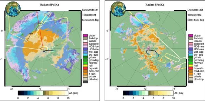
Since our main focus is to compare the in-situ measurements on board the aircraft and the SPolKa radar data, the area of interest here is limited to a circle of 150 km of diameter around the radar, as illustrat-ed inFig. 1.

2.2. Spolka classification

The ground-based SPolKa is an S-band (10.62 cm wavelength) and Ka band (8.6 mm wavelength) dual-polarization, dual-wavelength, scanning Doppler weather radar developed by the NCAR (National Cen-ter for Atmospheric Research;Lutz et al., 1997; Keeler et al., 2000; Farquharson et al., 2005). The SPolKa is transportable and can be de-ployed in remote locations. During DYNAMO, it was located on the Addu Atoll in the Maldives (73.10277 E, 0.63045 S) from the 1st of Oc-tober 2011 to the 15th of January 2012, about 8 km north of Gan Inter-national Airport. It collected radar data 24 h a day, 7 days a week, and was operational during 96% of the deployment time.

The S-band radar alternately transmits pulses that are horizontally polarized with pulses that are vertically polarized. This facilitates full dual-polarization radar measurements including horizontal reflectivity (Zh), differential reflectivity (Zdr), specific differential propagation phase (Kdp)— which is derived from the total differential phase (Φdp), Linear Depolarization Ratio (LDR), and the correlation coefficient (ρhv). These variables depend on the microphysical characteristics of hydrometeors such as the size, shape, orientation, phase (liquid or solid), and bulk density. The Zhis a measure of the power backscattered by the particles within the radar volume. It is proportional to the sixth moment of the particle size distribution when the particles are small compared to the wavelength (less than about 1 cm for S-band). This makes Zhvery sensitive to particle size and dominated by the largest particles in the radar volume. The Zdris the ratio of power return in the horizontal and vertical polarizations. The Zdrcan be interpreted as the reflectivity-weighted mean axis ratio of the particles. The LDR is the ratio of the vertically polarized backscattered power from a horizon-tally polarized transmitted wave to the horizonhorizon-tally polarized backscattered power. The Kdpis the difference in phase per kilometer of the received horizontal and vertical polarized waves. Theρhvis the complex correlation between the horizontal and vertical polarized sig-nals. Complete descriptions of the variables and their interpretation can be found inVivekanandan et al. (1991, 1999),Straka et al. (2000)

There are several algorithms that combine the information from the various dual-polarization measurements and temperature data to estimate the most likely particles responsible for the radar observations (Vivekanandan et al., 1991, 1999; Straka et al., 2000; Liu and Chandrasekar, 2000; Keenan, 2003; Dolan and Rutledge, 2009). The Par-ticle Identificator (PID) algorithm used in this study (Vivekanandan et al., 1999) is based on fuzzy logic. During DYNAMO the inputs were the dual-polarization variables, the temperature from soundings every 3 h on Gan Island, and two derived inputs, namely the standard devia-tions of ZdrandΦdpcomputed overfive range bins. Although the PID ran in real-time during the experiment, it was rerun in post-analysis in order to use the sounding closest in time. This results in a maximum lag of 1.5 h between the time of the sounding and the PID. The algorithm outputs eight separate classes of frozen hydrometeors (there arefive grades of rain leading to thirteen hydrometeor categories) and four non-meteorological categories for insects, clutter, receiver saturation, and second trip echoes.

“Horizontal Oriented Small Ice”, “Non-Oriented Small Ice”, “Dry Ag-gregates” (dry-agg) and “Wet Aggregates” (wet-agg), and “Graupel/ Rimed Aggregates” (gr/rmdag) will not necessarily be very well distin-guished usingρhvor LDR. The Zh, Zdrand Kdpare the measurements that will provide most of the information about size and orientation of these observed particles. There is certainly an overlap between the radar sig-natures of the different categories, however the algorithm is designed with the goal of identifying the most likely particles. The“Horizontal Oriented Small Ice” is made of small ice that could include pristine ice crystals falling with their major axis aligned horizontally due to aerody-namic forces. These include needles, columns, plates and dendrites. Small combinations of particles that fall horizontally and have small Zh values would also be included in the“Horizontal Oriented Small Ice” category. The“Horizontal Oriented Small Ice” category is therefore de-scribed by low Zhvalues and high Zdrand elevated Kdpvalues. The “Non-Oriented Small Ice” is made of non-oriented small ice category that has similar Zhvalues as the horizontal small ice, but without the Zdrand Kdpindicating a horizontal orientation. The two“Aggregates” categories are more likely a generic aggregate-type that represent larger particles and therefore larger Zhvalues. Graupel and rimed aggregates

have even higher Zhvalues still. In mixed phase conditions the Zdr,ρhv and LDR signatures are quite strong and more easily identified.

The naming convention for the various species is slightly different from the one originally used during thefield campaign in Gan and was elaborated during the post-analysis rerun through personal com-munication with the University of Washington, so it is very close to the naming convention found inRowe and House (2014).

Data quality is crucial to obtaining physical results from the PID algo-rithm. The data quality procedures for the DYNAMO experiment includ-ed calibration of horizontal reflectivity (Zh) and differential reflectivity (Zdr), verification of the pointing and ranging, and ensuring a flat and level system. The Zhcalibration was verified and monitored using solar scans, a test signal injected into the receiver, and the self-consistency calibration technique ofVivekanandan et al. (2003). The Zdrcalibration was achieved using vertical pointing scans in steady, light precipitation at various times throughout the project. The pointing and range measurements were verified using the known location of fixed towers that were detected by the radar. Because physical settling can occur during deployments, the radar pedestal was routinely verified to be level (and adjusted if needed) throughout DYNAMO.

2.3. Microphysics catalog

During the campaign in Gan, ice crystal observations were per-formed using a new generation of optical array probes with respect to the classical 2D-C and 2D-P. First, the 2D stereo probe (2D-S) from SPEC Inc. (Lawson et al., 2006) recorded images of particles from 10 to 1280μm with 10 μm resolution. Second, the Precipitation Imaging Probe (PIP) from Droplet Measurement Technologies provided images in the 100 to 6200μm range with a 100 μm resolution. To complete the set of instruments, the Cloud Particle Imager (CPI) probe (Lawson et al., 2001) provided images from 25 to 800 μm with a 25 μm resolution.

Sizes of the 2D images of the hydrometeors were corrected using the correction of the pixel resolution from the in-situ true air speed (Baumgardner and Korolev, 1997). In order to correct for possible

Fig. 1. SPol-Ka horizontally polarized reflectivity (in dBZ) at ~2.5° elevation for the two case studies. On the left-hand side the 06:15:31–06:20:31 UTC sequence on the 27th of November and on the right-hand side the 07:30:32–07:35:32 UTC sequence on the 8th of December. The plane trajectory is indicated over the reflectivity. The color of the plane trajectory is altitude-coded and the correspondence is given in the bottom color bar. The light green region shows exactly where the plane is located between the“start” (Start) and the “end” (End) of the sequence. Range rings are set every 50 km, centered on the radar location.

shattering effects, the rejection correction technique proposed byField et al. (2006)was also applied.

Characterization of scattering at 89 and 157 GHz is ultimately the goal of the MT algorithm validation effort. In this study only the PIP will be used since the larger “precipitating” particles are those impacting these frequencies the most. From the collected data, catalogs of the 2D images of the PIP were built into two categories. Thefirst cat-alog includes prints of 2D images which are within the size range 2–4 mm. As the number of particles recorded by the PIP is large in this size range (sometimes exceeding 5000 counts per second), a subset of particles is randomly chosen, and the probability that a given particle is selected increases quasi linearly with its size. The second catalog dis-plays the 2D images of particles which are larger than 4 mm, in which case all particles are printed. Particles of a size smaller than 2 mm are processed but not represented in the catalog because their size makes it dif_{ficult to define their shape or species.}

3. Results

This section presents the coherence between the microphysical in-situ measurements and the PID classification obtained from the SPolKa radar data. The in-situ data were collected with the PIP probe on-board the Falcon-20. One of the reasons for using only the PIP in the present study comes from the fact the PIP was the only probe that oper-ated for both of the case study presented here. The resulting catalogs are then empirically compared with the PID provided by the SPolKa radar. Seventeen classes of hydrometeors do exist in the SPolKa PID classi fica-tion but we mainly worked with 10 of them in the analysis of the parti-cles presented in theTables 1 and 2. The whole volume explored by the radar is classically divided into radar gates and each of these gates, when there is enough return signal gets a PID.

In order to describe and characterize the microphysical in-situ data from the catalogs they are visually compared with the“Meteorological Classification of Snow Crystals” introduced byMagono and Lee, 1966

and then improved byKikuchi et al., 2013. The Magono and Lee classi fi-cation has been widely used to describe snow crystal shapes. Neverthe-less their classification was incomplete and did not include for instance the aggregates “A” type and “H” type (“other solid precipitation groups”), proposed byKikuchi et al., 2013.

To compare the microphysical in-situ measurements with the PID, it isfirst necessary to co-locate the trajectory of the Falcon-20 with the nearest radar gate of the SPolKa. Since the PID is non-numerical infor-mation it is not possible to average the particle types within a volume or over time. To overcome this difficulty, the proportion of each radar PID met by the aircraft along its trajectory is represented as a pie-chart which wedges represent the proportion of each species. If the air-craftflies through two radar gates with two different PIDs, the pie-chart will come out as divided between two colors, etc. The proportion of each species is indeed simply the ratio between the number of radar gates containing a given species divided by the total number of radar gates over a given time.

3.1. Case study

Two situations that offer very different features in terms of convec-tive activity will be studied. Thefirst case on the 27th of November 2011 was observed during an active MJO episode. A thorough descrip-tion can be found on the DYNAMO-EOL website (http://catalog.eol. ucar.edu/cgi-bin/dynamo/report/index). During the 26–27th of Novem-ber, a series of small squall lines passed over Gan. These lines were short-lived with a small stratiform part. On the 26th at 22:00 UTC a se-ries of convective cells organized into a NE–SW line. The convective ac-tivity strengthened with time and a substantial stratiform region developed. In the early hours of the 27th, two other short-lived squall lines passed through the stratiform area, north of the radar at 03:30 and 08:00 UTC. The Falcon-20flight #110045 took place when the

stratiform was still fully developed, prior to the formation of the convec-tive line that occurred after 08:00 UTC. The aircraft took off at 05:34 UTC (09:34 MVT_{— Maldives Time) to sample the stratiform region. The} flight path circumvented heavy rain, north–north-east of the radar at about 75 km (not shown) and reached the target roughly half an hour later. From 06:05 to 07:15 UTC, the aircraft performed a series of hippodrome(race-track)-shapedfigures within the same stratiform re-gion (SeeFig. 1a).

During thefive-minute sequence from which is extracted the PPI shown inFig. 1a, the aircraft was located north–north-west of the radar along the light green line, between the (Start) and (End).

Each passage was completed at a different altitude: 9.5, 8.0, 6.5 and 4 km with a brief passage at 5 km. This strategy allowed us to have a se-ries of co-located data between the SPolKa PID and the in-situ sensors at different altitudes. Afterward the aircraft went north-west of the radar, outside of the 150 km region to sample a developing cell and returned to Gan, landing at 08:50 UTC (13:50 MVT).

The second case presented here took place on the 8th of December 2011 as a coordinatedflight with the NOAA-P3 aircraft and sampled ac-tive but disorganized convection. Theflight started at 06:05 UTC (10:05 MVT) andfirst headed toward the south-east of Gan to sample a series of small isolated cells located between 100 and 150 km from the radar. Co-located data at the edges of the radar domain were collected at about 07:00 UTC in an isolated weak cell. A long ferry took the Falcon-20 to the north–north-west of the radar where a larger stratiform region was ex-plored. This region later saw the development of new active cells. Co-located data were acquired during afirst pass at 9.5 km at 07:00 UTC and again between 07:50 and 08:20 UTC in this region at two different altitudes, 8 and 6.5 km (illustrated onFig. 1b). The Falcon-20 then_flew back toward Gan and performed a 8-shapedflight pattern between 08:30 and 08:45 UTC at about 25 km in the south-west quadrant of the radar at 6.5 km. Unfortunately, this latter pass was too close to the radar to get any co-located data. Indeed, due to the beam elevation upper limit (11° in the surveillance scans), there is a cone without data right above the radar. The Falcon-20 returned to Gan at approxi-mately 08:57 UTC (13:57 MVT).

3.2. Co-location between microphysics and SPolKa PIDs

Co-location of the in-situ data with the radar data is critical for the comparison. The in-situ data were positioned using the on board GPS system of the Falcon-20. The aircraft position is given with a 1 Hz fre-quency and since the aircraft's average speed was close to 558 km·h−1, the aircraft moves by about 155 m between two positions. It should be noted that the aircraft velocity depends on its altitude: slower at lower altitude and faster at higher altitude. In addition to the aircraft position in latitude–longitude, the GPS system provides an altitude with the same frequency. Finally, the in-situ data are timed by the GPS clock.

The radar data are located using a cylindrical system where each radar gate is positioned relative to the radar itself using an elevation/az-imuth/distance coordinate system. The radar sampling strategy is made of various sequences combining PPIs and RHIs. In this study we used only the PPIs for practical reasons. The RHIs cover a very limited sector of the aircraftflight path. Therefore to maximize the amount of co-located data it is more efficient to use the PPIs. The radar performs a sur-veillance sequence every 15 min. Each sequence is made of eight PPIs at different elevations roughly 0.6, 1.6, 2.6, 3.6, 5.2, 7.0, 9.1, 11.2°. There is an average of 360 rays per sweep and 979 gates per ray. The radar gates are 150 m deep along the ray and the width and height are approximat-ed with the simplified formula R ∗ Θ where R is the radial distance to the radar in km andΘ is the beam width in radian. The latter is given as 0.91°, meaning the last gate in a ray has a diameter of approximately 2.33 km at 146.85 km.

The co-location is performed by looking for the radar gate that con-tains the aircraft at a given moment. On the one hand, the radar latitude,

longitude and altitude are 73.10277 E, 0.63045 S and 10 m respectively. On the other hand, every second, the aircraft latitude, longitude and al-titude are given by the GPS. From the laal-titude and longitude of the radar and the aircraft, using the haversine formula, the down-range (geodetic distance) and azimuth of the aircraft (with the radar at the apex) are computed. The down-range and the aircraft altitude are then used to compute the slant-range using the cosine formula in the triangle made of the aircraft, the Earth center and the radar. Finally, the height/distance formula proposed byDoviak and Zrnić (1993)is used to compute the elevation of the aircraft as seen from the radar. With the known azimuth, elevation and slant-range (and the beam aperture) the radar gate eventually containing the aircraft can be determined.

Since aflight lasts about 3 h and there are four radar sequences per hour, the wholeflight is covered by twelve sequences. If a strict time matching was sought, very few co-location matches would be found. In order to relax this constraint, once the geometric aspect is addressed, the PID from the closest sequence in time is used for that particular air-craft position with a maximum accepted time lag of 7 min.

A certain amount of error is expected to remain in the co-location process due to GPS errors (particularly in the altitude), clock errors and encoder uncertainties in the radar pointing system and referencing. It is hard to estimate these remaining uncertainties but calculation sug-gested that the position is known within a precision of one ray and a couple of radar gates. Furthermore this precision is dependent on the distance to the radar since all references are based on angle–distance

relationships. The reached precision has to be kept in mind in the com-parisons presented hereafter.

As it is in the present study, the frequency at which the co-location is performed is independent of the radar volume size (i.e. in-dependent of the distance between the radar and the aircraft). It is also to be noted that the beam-bending is only accounted through theDoviak and Zrnić (1993)formula and that the Earth is assumed spherical.

Fig. 2a shows an example of the respective Falcon-20flight pattern and of the SPolKa PID image for a PPI at elevation 2.6° similarly to

Fig. 1a. The images are also extracted from the 06:15:32–06:20:32 UTC radar sequence on the 27th of November. The PID classification is strongly structured by the temperature profile and this shows clearly on the PPI image of this large stratiform area where particles are orga-nized in concentric distributions. One must remember that in the PPI ge-ometry the distance to the radar is roughly equivalent to an altitude proportional to the elevation angle. The area at the center of the image is occupied by a mixture of“Light Rain” (lt-rain) and “Drizzle” with some“Cloud Drops” (cld-drop) near the radar. The low elevation on the image (2.6°) gives a well marked layer of“Wet Aggregates” be-tween 75 and 110 km of the radar, which correspond in altitude from ~3.5 to 5 km. Embedded in the“Wet Aggregates” area are a number of isolated radar gates classified either as “Graupel with Rain” or “Graupel with Rimed Aggregates”. Above this “Wet Aggregates” layer, a layer of “Dry Aggregates”, “Non-Oriented Small Ice” and “Horizontal Oriented

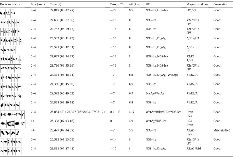
Table 1

Catalog images and associated PID for a selection offlight #110045 on the 27th of November. First column are images from PIP probe. The vertical bar is 7 mm. The second column is the size range referring to one of the two in-situ catalogs. Third column is the time in second since midnight and in hh:mm:ss UTC, fourth column is the temperature at theflight altitude in ° Celsius. Fifth column is theflight altitude in km. Sixth column is the PID as given by SPol-Ka classification system at the same location where “HOS-Ice” for “Horizontal Oriented Small Ice”, “NOS-Ice” stand for “Non-Oriented Small Ice”, “DryAg” for “Dry Aggregates”, “WetAg” for “Wet Aggregates”, “Drizz” for “Drizzle”, “ClDr” for “Cloud Drops” and “Gr” for any of the “Graupel”-type mixture. For each sample (line), the particle “Graupel”-types are given by order of importance. Seventh column is a matching particle “Graupel”-type as it can be found inMagono and Lee (1966)and Kikuchi et al (2013). Eighth column gives an indication on the agreement quality between the PID and the catalog.

Particles in situ Size (mm) Time (s) Temp (°C) Alt (km) PID Magono and Lee Correlation

2–4 22,047 (06:07:27) −28 9.5 NOS-Ice/HOS-Ice CP5/S3 Good 2–4 22,656 (06:17:36) −16 8 NOS-Ice R2d/CP1a CP5 Good 2–4 22,787 (06:19:47) −16 8 HOS-Ice R2d/CP1a CP5 Good

2–4 23,503 (06:31:43) −16 8 NOS-Ice/DryAg A/R1c/H3 Good

2–4 23,521 (06:32:01) −16 8 NOS-Ice/DryAg A/R1c H3 Good 2–4 23,667 (06:34:27) −16 8 HOS-Ice/NOS-Ice R2/R1 A/H3 Good 2–4 23,726 (06:35:26) −16 8 NOS-Ice/HOS-Ice R2d/CP1a CP5 Good

2–4 24,321 (06:45:21) −7 6.5 NOS-Ice/DryAg (WetAg) R1/R2/A Good

2–4 24,330 (06:45:30) −7 6.5 NOS-Ice R1/R2/A Good

2–4 24,542 (06:49:02) −7 6.5 DryAg/WetAg R1/R2/A Good

2–4 24,598 (06:49:58) −7 6.5 NOS-Ice R1/R2/A Good

2–4 25,084b T b 25,397 (06:58:04–07:03:17) 0–(+)3 4–5 WetAg/Drizz/ClDr/NOS-Ice Drop H2a Good N4 25,398 (07:03:18) 0 4.5 WetAg/NOS-Ice H2a Drop Good N4 25,477 (07:04:37) −2 5.5 NOS-Ice A2/A3 H2a Misclassified 2–4 26,583 (07:23:03) −14 8 NOS-Ice R2d/CP1a CP5 Good

Small Ice” can be seen from 110 to 150 km from the radar (correspond-ing to altitudes from ~5 to 7 km). In that layer, the distribution between the three species is more complex and strongly depends on the consid-ered region. South-east of the radar,“Horizontal Oriented Small Ice” clearly dominates while in the eastern half,“Non-Oriented Small Ice” dominates with a few areas of“Dry Aggregates”. North of the radar, where the aircraft isflying at that moment, a well-defined layer of “Dry Aggregates” can be observed. This region where the aircraft flew a series of hippodrome/race-track shaped descent is indeed where ac-tive convection and strong reflectivities were observed in the (not shown) previous PPIs. This is also the location of the highest reflectivity values inFig. 1a (~40 to 45 dbZ) and where most of the“Graupel” types are found as described below.

Fig. 3shows the vertical cross-section of the SPolKa PID for the same sequence, along the red line ofFig. 2a (azimuth 350°). As for theFig. 1a, the size of the radar gates is close to their actual scale. The position of the aircraft at about 100 km from the radar and about 8 km altitude is indi-cated by a green star. As usual with PID-type classifications, the 0° iso-therm is splitting the atmospheric column between ice and liquid precipitation. The larger radar gates as one goes further from the radar increase the uncertainty in terms of separating liquid from solid parti-cles. The“Wet Aggregates” category is found near the melting layer. De-pending on the distance and thus the resolution, this category can be found either above or below the freezing level, which is likely to be an artifact due to the radar sampling volume. A spot of“Rain–Graupel” mixture can be seen between 75 and 110 km right above a moderate rain layer where the convective activity took place. At that particular moment the aircraft is seenflying between two PPIs, below a mixture

of“Horizontal Oriented Small Ice” and “Non-Oriented Small Ice” and above a layer of“Dry Aggregates”.

Fig. 2b illustrating the 8th of December morningflight, offers very different features in terms of the PID_{field structure. As for}Fig. 1b, the re-flectivity field contrasts with the very large stratiform area on the 27th of November. Thisflight is one of the best matches in terms of co-location between the Falcon-20 and the radar domain. At the time of the image, the aircraft was investigating the remnant of an active area north of the radar while a more active line propagating to the east– north-east is located south of the radar, indicated by the presence of the“Heavy Rain” category corresponding to reflectivities of about 45 to 50 dbZ inFig. 1b. The general features of the PIDfield are consistent with the literature (e.g.Houze, 1993, among many others). First, the rain pattern is very consistent with core of“Heavy Rain” embedded in “Moderate Rain” areas which are in turn surrounded by “Light Rain” and“Cloud Drops”. The “Wet Aggregates” is encountered near the melt-ing layer which is around 4.5 km, about 70 km from the radar at eleva-tion 3.6°. A few spots of“Graupel with Rimed Aggregates” and “Rain– Graupel” can be seen at 100 km from the radar at azimuth 150° or at about 50 km from the radar in the NNE_{–NNW quadrant. Contrarily,} most of the ice phase is made of large areas of “Dry Aggregates” surrounded by“Non-Oriented Small Ice”. “Horizontal Oriented Small Ice” is found randomly above 6.5 km altitude which is roughly 100 km from the radar.

In order to estimate the agreement between the in-situ data and the SPolKa PID a limited number of short sequences were isolated for each of theflights. Since the aircraft position is known every second, the radar gate containing the aircraft is computed every second and its

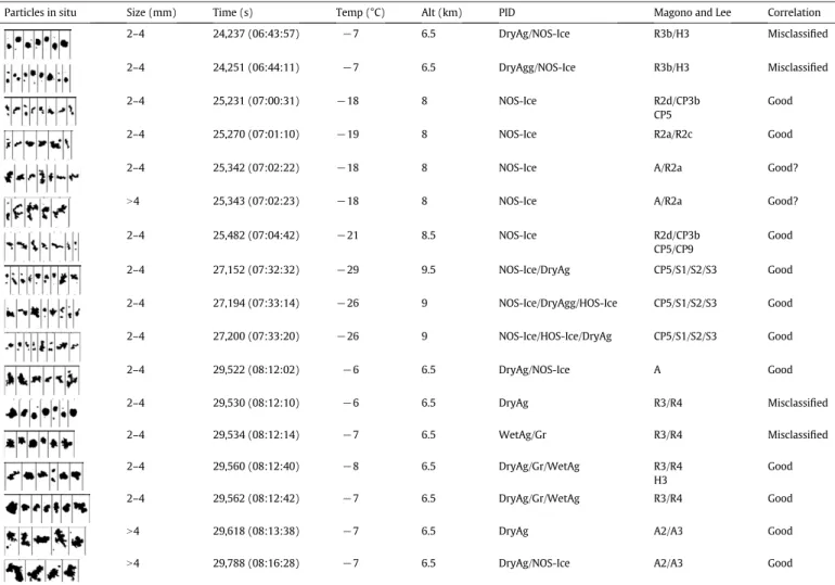
Table 2

IdemTable 1 but for the flight #110050 on the 8th of December.

Particles in situ Size (mm) Time (s) Temp (°C) Alt (km) PID Magono and Lee Correlation

2–4 24,237 (06:43:57) −7 6.5 DryAg/NOS-Ice R3b/H3 Misclassified

2–4 24,251 (06:44:11) −7 6.5 DryAgg/NOS-Ice R3b/H3 Misclassified

2–4 25,231 (07:00:31) −18 8 NOS-Ice R2d/CP3b

CP5

Good

2–4 25,270 (07:01:10) −19 8 NOS-Ice R2a/R2c Good

2–4 25,342 (07:02:22) −18 8 NOS-Ice A/R2a Good?

N4 25,343 (07:02:23) −18 8 NOS-Ice A/R2a Good?

2–4 25,482 (07:04:42) −21 8.5 NOS-Ice R2d/CP3b CP5/CP9 Good 2–4 27,152 (07:32:32) −29 9.5 NOS-Ice/DryAg CP5/S1/S2/S3 Good 2–4 27,194 (07:33:14) −26 9 NOS-Ice/DryAgg/HOS-Ice CP5/S1/S2/S3 Good 2–4 27,200 (07:33:20) −26 9 NOS-Ice/HOS-Ice/DryAg CP5/S1/S2/S3 Good 2–4 29,522 (08:12:02) −6 6.5 DryAg/NOS-Ice A Good 2–4 29,530 (08:12:10) −6 6.5 DryAg R3/R4 Misclassified 2–4 29,534 (08:12:14) −7 6.5 WetAg/Gr R3/R4 Misclassified 2–4 29,560 (08:12:40) −8 6.5 DryAg/Gr/WetAg R3/R4 H3 Good 2–4 29,562 (08:12:42) −7 6.5 DryAg/Gr/WetAg R3/R4 Good

N4 29,618 (08:13:38) −7 6.5 DryAg A2/A3 Good

PID is counted as“seen” by the aircraft. This simulates the aircraft's flight in a volume with spatial resolution that would be given by the radar gate size at that particular location. This way, the proportion of each species can be computed independently of the distance to the radar, even if the same radar gate can be accounted for more than once. The pie-chart representation shows the proportion of each species along the aircraft trajectory and is compared with the particle catalog described inSection 3.3.

3.3. Comparison of PIDs and in-situ catalog

Two short seven-minute sequences of co-located PID and airplane trajectory are presented here respectively forflights #110045 and #110050. Fig. 4shows the results of the co-location described in

Section 3.2for_{flight #110045 on the 27th of November for the SPolKa} sequence 06:30:32–06:35:32 UTC. The aircraft is 120 km north of the radar at an altitude of 8 km,flying along a north-east/south-west direction. The top and bottom axis on thefigure are the time in seconds since 00:00:00 and the UTC time respectively. The vertical axis is the altitude in km. The upper right thumbnail is a summary of theflight pattern with respect to the radar, with the green star indi-cating the position of the aircraft at 06:30:00 UTC (23400 s). Two

different pieces of information are displayed in thefigure. The first one is a pseudo vertical cross-section of the PID along the aircraft track. For every aircraft position (approx. every second), the radar gate containing the aircraft is found through the co-location process previously described. The radar gates that are geometrically below and above the aircraft are also selected without consideration for the time lag between the radar and aircraft clocks. Knowing that each PPI takes approximately 37.5 s, this gives us the amount of time between two“levels”. On top of this pseudo vertical cross-section is a series of pie-charts, representing the proportion of each species found in the aircraft's environment over a period of 10 s. Since some errors might remain in the co-location process, the pie-chart not only takes into account the current radar gate in which the aircraft is found to beflying, but also four neighboring gates: one further, one closer along the current radar ray, one in the previ-ous ray, and one in the next ray within the same PPI. This choice is ar-bitrary, meant to provide a more statistical sense of the local PID, knowing that sometimes the fuzzy logic algorithm can give a unique answer when in fact two species have very similar probability. This usually translates into a noisy PIDfield which should be reflected in the pie-charts. These pie-charts are compared with the in-situ cata-logs inTables 1 and 2.

Fig. 3. Vertical cross-section of the PID species from SpolKa corresponding toFig. 2a (and 1a), at azimuth 350°. Horizontal and vertical axis are respectively the distance to the radar and the altitude in km. Position of the plane when intercepting the vertical cross-section in distance and altitude is also indicated by a green star at 100 km from the radar and about 8 km altitude. The PIDs are the same as inFig. 2.

Fig. 2. Same asFig. 1but for the PID instead of the reflectivity. The various species provided by the classification algorithm are shown on the right-hand side scale (names are straightfor-ward except for:“supcoold”: Super Cooled Water, “NOS-ice”: Non-Oriented Small Ice, “HOS-ice” Horizontal Oriented Small Ice, “wet-agg”: Wet Aggregates, “dry-agg”: Dry Aggregates, “gr/ rain”: Graupel/Rain, “gr/rmdag”: Graupel/Rimed Aggregates, “hvy-rain”: Heavy Rain, “mod-rain”: Moderate Rain, “lt-rain”: Light Rain and “cld-drop”: Cloud Drops). The red line at azimuth 350° is the location of the vertical cross-section presented inFig. 3.

FromFig. 4, it can be seen that the various hydrometeor species are organized horizontally in homogeneous layers. First, a mixture of “Hor-izontal Oriented Small Ice” and “Non-Oriented Small Ice” is present above about 8 km. Second, a“Dry Aggregates” layer can be seen above a“Wet Aggregates” layer between 4 km and 7 km. Below the melting layer, a mixture of“Moderate Rain” and “Light Rain” occurs. Embedded in the“Wet Aggregates” layer a few radar gates containing some of the graupel mixtures can be locally observed.

This part of the system is decaying throughout the entireflight. The horizontal structure of the layers is a rather classic stratiform feature (e.g.Houze, 1993, among many others). The graupel presence is consis-tent with the earlier convective activity. This organization in horizontal layers tends to disappear from this point as the stratiform region dissi-pates after 06:45 UTC.

It can be seen that some gates are classified as “clutter” at 06:33:20 and 06:33:25 UTC and correspond to the back scattering signal from the Falcon-20 itself. This gives an indirect indication of the quality of the location of the aircraft in the radarfield. Whenever we had such an occurrence, the contaminated gates were disregarded.

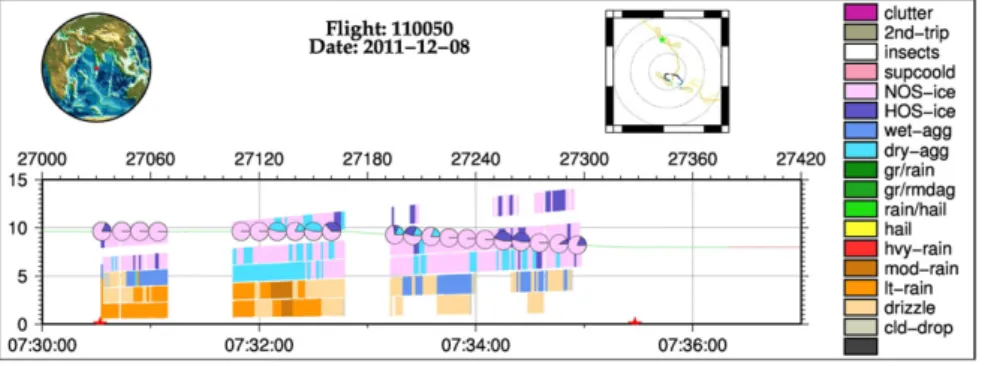
Fig. 5is similar toFig. 4except forflight #110050 on the 8th of De-cember for the SPolKa sequence of 07:30:32–07:35:32 UTC. The aircraft isflying north of the radar at about 100 km, in the large stratiform re-gion where active convection will later develop. The current pass starts at 9.5 km altitude andfinishes at 8 km altitude in an environment where there should be decaying convective cells and future active ones. Unlike the 27th of November case, this system is showing a clear evolution on the radar quick-looks (not shown) and seems to intensify during the flight. In terms of PID, the main difference between this case and the previous one is the lack of a clear layer of either“Dry Aggregates” or “Wet Aggregates”. The various ice/aggregate species are very mixed in the layers, with a majority of“Non-Oriented Small Ice”. Below the

freezing level, the species are a mixture of“Moderate Rain”, “Light rain” and “Drizzle”.

This case is made of transient cells, hence the distribution in horizon-tal layers is less pronounced. One striking feature is the lack of graupel-like PIDs in this supposedly more convectively active area. It was noted during theflight that, although the convection should be deep in the Gan area, the vertical velocities measured by the in-situ probes, or by any other means, were weak, which might explain both their transient character and the lack of denser species.

Tables 1 and 2present the comparison between the particle classi fi-cation by the SPolKa and the in-situ catalogs and then with Magono and Lee's Meteorological Classification of Snow Crystals. The first column presents a sample of the in-situ catalog from the PIP. The vertical bar is a size reference and is actually 7 mm high. The samples are randomly selected from the catalog to illustrate qualitatively the PID found by the radar. The second column shows from which of the two catalogs the particles were taken: either the 2–4 mm or the N4 mm (seeSection 2.3).

The third column is the time in seconds since midnight. This is not the precise time at which the particles were collected, but for technical reasons, it is the collection time of the last particle on the catalog line. In a well-populated environment, there is about 1 s per catalog line so the given time is within 1 s of the actual collection time. In poorly populated environments, there can be a much larger amount of time between two successive catalog lines so the precision of the collection time of a given individual particle becomes much less precise. Nonetheless, whenever possible, the selected particles are always closest to the given time in order to minimize this uncertainty. The fourth column is the in-situ temperature in Celsius as measured by the aircraft and thefifth column is the average altitude in km as reported by the aircraft. In the sixth col-umn are the various species proposed by the PID from SPolKa (the spe-cies found in the pie-chart diagrams as presented inFig. 4). The seventh

Fig. 4. Along-track vertical cross-section of the PID species (same one as inFig. 2) on the 27th of November between 06:30 and 06:37 UTC matching the radar sequence 06:30:32–06:35:32 UTC. The upper horizontal scale is second since midnight, lower horizontal scale is the time UTC. The vertical axis is the altitude. The green dotted line is the planeflight path. Vertical size of the radar bins are represented at scale. The two red stars at altitude 0 are respectively the beginning and the end of the radar sequence. The green star in the upper-right-hand side thumb-nail is the location of the plane at 06:30 UTC. The“clutter” at 06:33:20 UTC is the back-scattered signal of the Falcon. The pie-charts at the flight altitude are the proportion of each species at theflight location integrated over 10 s and in the four neighboring radar bins.

column suggests a selection of matching crystal type fromMagono and Lee's classification (1966)andKikuchi et al. (2013). The eighth column concludes on the relevance of the agreement between the PID classi fica-tion and the PIP samples.

Table 1(flight #110045 on the 27th of November) shows a few se-lected samples along the_{flight pattern when the aircraft passes} repeat-edly at approximately the same location at various altitudes. There is a good consistency between the PID and the in-situ crystals images.

At the highest pass (9.5 km,−28 °C) small crystals were found by the in-situ probes. Their sizes and shapes are compatible with the com-mon idea one has of a PID classified as “Non-Oriented Small Ice” and/or “Horizontal Oriented Small Ice”. As stated above, in order to identify more precisely the particles from the two PIP catalogs, these images were matched with the classifications proposed byMagono and Lee (1966)and followers, based on size and shape, but also on temperature range. These small crystals, for temperature ranges below_{−25 °C, are a} good match in theMagono and Lee (1966)but also in theWeickmann (1948)classifications, for the S2 type (“scale like side planes”) and S3 (“combination of side planes, bullets and columns”). These particles could also match the CP5 (“irregular combination of column and plane”) proposed byKikuchi et al. (2013)and made of snow crystal that are a combination of columns, bullets and crossed plates.

Thefirst pass at 8 km (−16 °C, i.e. 06:17:36 UTC on a SW–NE trajec-tory) shows relatively small particles with irregular shapes. The second pass at 8 km (−16 °C, i.e. 06:31:43 UTC on a NE–SW trajectory about 10 km south of thefirst pass) exhibits larger particles mixed with a few smaller crystals that could be regarded as“ice pellet crystal type” (H3). Some of them are more clearly aggregates mixed with more com-plex shapes and properly labeled as a mixture of“Dry Aggregates” and “Non-Oriented Small Ice” (e.g. 06:31:43 UTC). Given their sizes and shapes and with temperature between−3.9° and −17.9 °C, in the

Kajikawa et al. (1980) classi_{fication, a matching type is the R1a} (“rimed needle crystals”). Some of the PIP images could even be a com-bination of R1a type crystals or eventually CP1 type crystals (“column with plates”). The latter are indeed often found around −20 °C and their characteristic size is about 1 mm. The Cloud Particle Imager data available for thisflight (not shown), quite clearly show “hexagonal plates” type (P1a) and “ice pellets” type (H3) that could easily match the“very small round” (relatively to the PIP resolution) particles seen by the PIP around 22787, 23,503 and 23,521 s.

A clear difference in particle size can be noted between these two passes at 8 km (06:17:36 UTC and 06:31:43 UTC). This second leg seems to be mostly made of“Dry Aggregates”. The latter is difficult to distinguish from the“Non-Oriented Small Ice” based on size only, but the crystals offer a more regular shape. The type A (“aggregates”) of

Kikuchi et al. (2013)that covers the size range between the single crys-tal and combination of single cryscrys-tals could also account for these larger particles.

The pass at 6.5 km (−7 °C) exhibits much larger particles as the temperature increases. It seems that these are mostly combination of various crystals made of columns and plates. Although the temperature has changed from−16 °C to −7 °C between this pass and the previous one, the general particle shapes are similar. The PID shows mainly a mixture of“Dry Aggregates” and “Non-Oriented Small Ice” which are consistent with the in-situ. It also shows some_{“Wet Aggregates”} which is not shown by the PIP catalogs (about 06:45:21 UTC) and are not compatible in terms of temperature. When looking more closely at the geometry for this particular leg, it is likely that the radar resolution (the aircraft is between 100 and 140 km from the radar) is encompassing the whole bright band and some of the frozen layers aloft and the sharp transition between dry and wet particles cannot be rendered accurately.

There is a short pass near and below the 0 °C isotherm, within the bright band, with data collected at 4 km (3 °C) and at 4.5 km (0 °C). In the catalog, some quasi-spherical particles could be identified as “Wet Aggregates” or even already drops.Kikuchi et al (2013)propose an

additional crystal with respect to the originalMagono and Lee (1966): the H2 type (“sleet particles”) whose size ranges from 1 to 10 mm. These are usually a mixture of rain and snow for which it is dif_{ficult to} assess the degree of melting.

The last examples are taken at 5.5 km (−2 °C) and 8 km (−14 °C and_{−17 °C) but at a different location, closer to the radar while the} air-craft was ferrying back. The results, both from the PID and from the in-situ, are very consistent with the previousfindings, with presence of “Dry Aggregates” and “Non-Oriented Small Ice”. Depending on the alti-tude and/or temperature, the in-situ images show more elongated par-ticles that are a good match for the “Non-Oriented Small Ice” or smoother/uniform particles that correspond more to“Dry Aggregates”.

Table 2is the same asTable 1but for the #110050flight on the 8th of December. As seen inFig. 5, the vertical distribution of the particles is much more random, with little organized layering due to the more convectively active and more transient nature of the cells. A majority of the samples shown are taken either at 6.5 km (−6 °C) or 8 km (−18 °C), with an example at 9.5 km (−29 °C), two at 9 km (−26 °C), and one at 8.5 km (−21 °C). The “Non-Oriented Small Ice” and“Dry Aggregates” are the most present and match very nicely the in-situ images.

At 06:43:57 and 06:44:11 UTC, the samples collected by the PIP at thefirst 6.5 km pass seem too spherical to be “Dry Aggregates”. This is a good example of disagreement between the two instruments. In the

Kikuchi et al. (2013)classification these could be R3 type (“graupel-like snow”) or H3 type (“ice pellets”).

At 8 km (−21° b T°C b −18 °C) the radar sees mostly “Non-Oriented Small Ice”, which seems coherent with the PIP measurement. Some par-ticles look like the CP9 type (“seagull”) made of two needles wings and proposed byKikuchi et al. (2013). These are supposedly found around −25 °C and are supposed to fall continuously during a short time interval.

For theflight leg between 9 and 9.5 km there is a good agreement between the PID and the in-situ samples. The temperature ranges from−26 °C to −29 °C and the CP5/S1/S2/S3 types ofMagono and Lee (1966)already presented inTable 1do match the PIP images.

Various types of“Graupel” mixture PID are found at 6.5 km altitude at 29,534, 29,560, and 29,562 s, matching the graupel found in the in-situ catalog. The latter appear indeed smoother than the“Wet Aggre-gates”, but offering some structure on their perimeter that distinguish them from water drops, although the difference with drizzle drops or rain drops (not shown) is not always obvious.

To summarize the previous discussion inTables 1 and 2(and other comparisons not shown), it seems that radar PID is consistently associ-ated with the same type of particles most of the time. The“Horizontal Oriented Small Ice” type is always found above 8 km and at tempera-tures of−16 °C or colder.

“Non-Oriented Small Ice” is usually associated with crystals of com-plex and variable shapes, generally elongated, with rough contours. Most of the time these are in the 2–4 mm size category and found at al-titudes equal or above 8 km. Unfortunately, the in-situ probes cannot give any information about particle orientation because the probe sys-tem and the aircraft itself can generate a very turbulent environment. The ice particles tend to increase in size as altitude decreases, becoming “Dry Aggregates”. Generally what the PID defines as “Dry Aggregates” corresponds to particles similar in shape to the“Non-Oriented Small Ice” but of larger size and with a slightly less elongated shape.

The_{“Wet Aggregates” type in the PID appears to be consistently} round particles with irregular but smooth edges. The various“Graupel” (essentially“Graupel with Rain” or “Graupel with Rimed Aggregates”) types in the PID appear even rounder than the“Wet Aggregates” type in the in-situ data and are found near the melting level at 6.5 km alti-tude. These graupel seem very close to the R4a/R4b (hexagonal grau-pel/lump graupel) type ofMagono and Lee (1966).

Only one example of warm in-situ microphysics is found between 06:58:04 and 07:03:17 UTC offlight #110045. A mixture of “Cloud

Drops”, “Drizzle”, “Non-Oriented Small Ice” and “Wet Aggregates” is given by the PID. If the two former species seem likely to be correct, and the last one seems possible, the_{“Non-Oriented Small Ice” is unlikely} at this altitude. But it is true that some of the in-situ particles found by the PIP probes do look very much like the“Non-Oriented Small Ice” type found much higher in altitude.

Several noticeable exceptions can be found. First, at 24,542 s (06:49:02 UTC) onflight #110045, a mixture of “Dry Aggregates” and “Wet Aggregates” is identified by the PID, while the presence of “Wet Aggregates” can be difficult to see in the in-situ images. However, the pie-chart in this region (not shown) shows a majority of“Dry Aggre-gates” and a small fraction of “Wet Aggregates”. As stated above, this is likely to be a spatial resolution problem from the radar which is un-able to catch the sharp transitions of the near melting layer at such a dis-tance. Second, at 24,237 s (06:43:57 UTC) and 24,251 s (06:44:11 UTC) of_{flight #110050, the PID gives a mixture of “Dry Aggregates” and} “Non-Oriented Small Ice” when the in-situ shows either warm particles or even graupel-like particles. At that time the aircraft is about 75 km from the radar, right at the upper part of the gap between two PPIs. The lower PPIs (not shown) contain a mixture of“Wet Aggregates”, “Drizzle” and “Cloud Drops”. Third, around 29,530 s (08:12:10 UTC), where some very round particles are improperly identified as “Dry Ag-gregates” when they look like either “Wet Aggregates”, hexagonal grau-pel, or lump graupel (type R4a or R4b inMagono and Lee, 1966). In this region, the pie-charts (not shown) are clearly“Dry Aggregates” but they shift to half“Dry” half “Wet Aggregates” and then to a mixture of “Wet Aggregates” and “Graupel”. Furthermore, the aircraft is again at the edge between two PPIs and the lower PPI is mainly of“Wet Aggregates”. Last, a few seconds later at 23,534 s (08:12:14 UTC), graupel or perhaps graupel-like snow (type R3c ofMagono and Lee, 1966) is improperly la-beled as“Wet Aggregates”. It is hard to tell if these exceptions are relat-ed to co-location problems or inderelat-ed misclassifications by the PID because the given examples are sparse. Nonetheless, one might notice that the supposedly more turbulent environment of the 8th of Decem-ber seems to lead to more misclassifications than the much more strat-iform case of the 27th of November.

It is important to keep in mind that the comparisons between the in-situ images and the various classifications fromMagono and Lee (1966)

orKikuchi et al. (2013)are not necessarily exhaustive and will require further work. In particular, these classifications were established either in Japan or in polar regions while we are dealing here with tropical oce-anic conditions.

4. Conclusion

The idea here would be to build a typology of particles habits as a function of life cycle of convection, large scale environment conditions, stratiform vs. convective etc. using ground based polarimetric radar. This typology is to be used further to set an appropriate ice parameter-ization in a radiative transfer model with spaceborne microwave-based rain retrieval algorithm development in sight. To be able to build such a typology, the particle classification needs first to be consolidated against some reference. The present paper analyzes the consistency between the Particle Identificator proposed by the SPolKa system and the in-situ measurements performed by SAFIRE Falcon-20 during two_flights of the Megha-Tropiques Algorithm Validation, phase II, exercise. This campaign took place in Gan (Maldives) while the CINDY–DYNAMO campaign looked at the relationship between MJO and convection in the Indian Ocean.

Every 15 min the SPolKa performed afive-minute sequence of height PPIs at various elevations. An effort for pre-processing those data, with very precise pointing and calibration, was conduced at NCAR. The PID classifications were then computed in the specific cylin-drical geometry of the radar. The Falcon-20 trajectory was re-projected within the radar volume and every second of the aircraftflight was lo-cated (when possible) within a radar gate of one of the various radar

sequences, based on distance and time criteria. Because the aircraft loca-tion and the radar pointing can be affected by uncertainties, even with the care taken, a method was designed to represent the proportion of each PID species in the aircraft vicinity. Since an average value is mean-ingless for a non-numerical variable, pie-charts were used to plot the proportion of each species every 10 s along the aircraft trajectory.

The co-location was validated with the aircraft's presence in the radarfield being identified in various sequences as “clutter” in a few radar gates.

The catalogs from the in-situ probes (Precipitation Imaging Probe) were visually matched with classical particle classifications like

Magono and Lee (1966)orKikuchi et al (2013), based on shape, size and the environment temperature. Then, the pie-charts representing the“averaged” PID were qualitatively compared with the particles from the catalogs. The agreement was good most of the time. In other words, the radar was able to correctly distinguish population of in-situ particles that were consistently found at various altitudes and locations in the rain systems. Both the shape and size, as well as density, seem to be properly sorted out by the PID when compared to the in-situ images. It was also found that the“Non-Oriented Small Ice” and the “Horizontal Oriented Small Ice” were not, most of the time, the same particles. Prob-ably because the environmental conditions are different when the par-ticles are oriented and non-oriented, the microphysical processes are different, leading to subtle differences in particle habits.

The more complex the particles' history, the more difficult it might be to identify the species from the catalogs. Partially melted and re-frozen particles, heavily rimed particles or aggregates with a strong 3D shape can be difficult to distinguish from the sole PIP 2D-images. The PID classes can then be hard to“validate”.

Only two cases were analyzed here. Unfortunately among the thir-teenflights of the Falcon-20 that took place during the DYNAMO cam-paign, only three were within the radar range. Nevertheless thesefirst comparisons are very promising. It is at this point difficult to assess whether or not the density and/or mass-diameter laws that could be de-duced from the in-situ data and those originating from the radar are consistent. The work will continue with similar studies being performed using the dataset from the Megha-Tropiques Algorithm Validation cam-paign in Niamey.

Since this effort is meant to be used in satellite product validation, the next stage will be to compare PIDs from various radars and bright-ness temperatures from MADRAS on Megha-Tropiques or TMI on TRMM to see if the particle types and their in_{fluence on the brightness} temperatures can be characterized.

Acknowledgments

This work and the various validationfield campaigns for Megha-Tropiques were funded by the Centre National d'Etudes Spatiales (CNES). The French Falcon-20 was deployed and operated during this campaign by the SAFIRE team.

References

Baumgardner, D., Korolev, A., 1997.Airspeed corrections for optical array probe sample volumes. J. Atmos. Ocean. Technol. 14, 1224–1229.

Bringi, V.N., Chandrasekar, V., 2001.Polarimetric Doppler Weather Radar. Cambridge Uni-versity Press.

Cassou, C., 2008.Intraseasonal interaction between the Madden–Julian Oscillation and the North Atlantic Oscillation. Nature 455, 523–527.

Desbois, M., Capderou, M., Eymard, L., Roca, R., Viltard, N., Viollier, M., Karouche, N., 2007. Megha-Tropiques: un satellite hydrométéorologique franco-indien. La Météorologie 57, 19–27.

Dolan, B., Rutledge, S.A., 2009.A theory-based hydrometeor identification algorithm for X-band polarimetric radars. J. Atmos. Ocean. Technol. 26, 2071–2088.

Doviak, R.J., Zrnić, D.S., 1993.Doppler Radar and Weather Observations. Academic Press. Farquharson, G., Pratte, F., Pipersky, M., Ferraro, D., Phinney, A., Loew, E., Rilling, R.A., Ellis, S.M., Vivekanandan, J., 2005.NCAR S-Pol Second Frequency (Ka-band) Radar. Pre-prints 32nd Conf. on Radar Meteor. AMS, Albuquerque, N.M.

Field, P.R., Heymsfield, A.J., Bansemer, A., 2006.Shattering and particle interarrival times measured by optical array probes in ice clouds. J. Atmos. Ocean. Technol. 23, 1357–1371.

Fiorino, S.T., Smith, E.A., 2005.Critical assessment of microphysical assumptions within TRMM radiometer rain profile algorithm using satellite, aircraft, and surface datasets from KWAJEX. J. Appl. Meteorol. Climatol. 45, 754–786.

Hou, A.Y., Kakar, R.K., Neeck, S., Azarbarzin, A.A., Kummerow, C.D., Kojima, M., Oki, R., Nakamura, K., Iguchi, T., 2014.The global precipitation measurement mission. Bull. Am. Meteorol. Soc. 95, 701–722.

Houze Jr., R.A., 1993.Cloud dynamics. International Geophysics Series 53. Academic Press. Kajikawa, M., Kikuchi, K., Magono, C., 1980.Frequency of occurrence of peculiar shapes of

snow crystals. J. Meteorol. Soc. Jpn. 58, 416–421.

Keeler, R.J., Lutz, J., Vivekanandan, J., 2000.S-Pol: NCAR's polarimetric doppler research radar. Proceedings of the International Geoscience and Remote Sensing Symposium. IEEE, Honolulu, Hawaii, pp. 1570–1573.

Keenan, T.D., 2003.Hydrometeor classification with a C-band polarimetric radar. Aust. Meteor. Mag vol. 52, 23–31.

Kikuchi, K., Kameda, T., Higuchi, K., Yamashita, A., 2013.A global classification of snow crystals, and solid precipitation based on observations from middle latitudes to polar regions. Atmos. Res. 132–133, 460–472.

Kummerow, C., Barnes, W., Kozu, T., Shiue, J., Simpson, J., 1998.The tropical rainfall mea-suring mission (TRMM) sensor package. J. Atmos. Ocean. Technol. 15, 809–817. Lawson, R.P., Baker, B.A., Schmitt, C.G., Jensen, T.L., 2001.An overview of microphysical

properties of Arctic clouds observed in May and July 1998 during FIRE ACE. J. Geophys. Res. Atmos. 106, 14989–15014.

Lawson, R.P., O'Connor, D., Zmarzly, P., Weaver, K., Baker, B., Mo, Q., Jonsson, H., 2006.The 2D-S (stereo) probe: design and preliminary tests of a new airborne, high-speed, high-resolution particle imaging probe. J. Atmos. Ocean. Technol. 23, 1462–1477.

Lin, H., Brunet, G., Derome, J., 2009.An observed connection between the North Atlantic Oscillation and the Madden–Julian Oscillation. J. Clim. 22, 364–380.

Liu, H., Chandrasekar, V., 2000.Classification of hydrometeors based on polarimetric radar measurements: development of fuzzy logic and neuro-fuzzy systems, and in-situ ver-ification. J. Atmos. Ocean. Technol. 17, 140–164.

Lutz, J.B., Rilling, B., Wilson, J., Weckwerth, T., Vivekanandan, J., 1997.S-Pol after three op-erational deployments, technical performance, siting experiences, and some data ex-amples. Preprints. 28th Conf. on Radar Meteorology. Amer. Meteor. Soc., Austin, TX, pp. 286–287.

Magono, C., Lee, C.W., 1966.Meteorological classification of natural snow crystals. J. of the Faculty of Sci.Hokkaido University, Japan (Ser VII, vol II, No 4).

Petersen, W.A., Rutledge, S.A., 2001.Regional variability in tropical convection: observa-tion from TRMM. J. Clim. 14, 3566–3586.

Rowe, A.K., House Jr., R.A., 2014.Microphysical characteristics of MJO convection over the Indian Ocean during DYNAMO. J. Geophys. Res. Atmos. 119, 2543–2554.

Schumacher, C., Houze Jr., R.A., 2003.Stratiform rain in the tropics as seen by the TRMM precipitation radar. J. Clim. 16, 1739–1756.

Straka, J., Zrnić, D.S., Ryzhkov, A.V., 2000.Bulk hydrometeor classification and quantifica-tion using polarimetric radar data: synthesis and relaquantifica-tions. J. Appl. Meteorol. 39, 1341–1372.

Vivekanandan, J., Adams, W.M., Bringi, V.N., 1991.Rigorous approach to polarimetric radar modeling of hydrometeor orientation distributions. J. Appl. Meteorol. 30, 1053–1063.

Vivekanandan, J., Zrnic, D.S., Ellis, S.M., Oye, R., Ryzhkov, A.V., Straka, J., 1999.Cloud micro-physics retrieval using S-band dual polarization radar measurements. Bull. Am. Meteorol. Soc. 80, 381–388.

Vivekanandan, J., Zhang, G., Ellis, S.M., Rajopadhyaya, D., Avery, S.K., 2003.Radar reflectiv-ity calibration using differential propagation phase measurement. Radio Sci. 38 (3), 8049.

Weickmann, H., 1948.The Ice Phase in the Atmosphere. Ministry of Supply, Millbank, London.

Yoneyama, K., Zhang, C., Long, C.N., 2013.Tracking pulses of the Madden–Julian Oscilla-tion. Bull. Am. Meteorol. Soc. 94, 1871–1891.