Aeroelastic flutter and divergence of graphite/epoxy cantilevered plates with bending-torsion stiffness coupling

AEROELASTIC FLUTTER AND DIVERGENCE OF GRAPHITE/EPOXY CANTI-LEVERED PLATES WITH BENDING-TORSION STIFFNESS COUPLING

by

STEVEN JAMES HOLLOWELL

B.S., United States Air Force Academy (1977)

SUBMITTED IN PARTIAL FULFILLMENT OF THE REQUIREMENTS FOR THE

DEGREE OF MASTER OF SCIENCE

IN

AERONAUTICS AND ASTRONAUTICS at the

MASSACHUSETTS INSTITUTE OF TECHNOLOGY January, 1981

Steven James Hollowell, 1980

The author hereby grants to M.I.T. permission to reproduce and to distribute copies of this thesis document in whole or in part.

Signature of Author_

Department of Aeronautics and Astronautics December 11, 1980 Certified by John Dugundji Thesis Supervisor Accepted by Wachman LIBRARIES / ARCHIVES Harold Y.

MMISlit agopartmental Graduate Committee OF TECHNOLOGY

AEROELASTIC FLUTTER AND DIVERGENCE OF GRAPHITE/EPOXY CANTI-LEVERED PLATES WITH BENDING-TORSION STIFFNESS COUPLING

by

STEVEN JAMES HOLLOWELL

Submitted to the Department of Aeronautics and Astronautics on December 11, 1980, in partial fulfillment of the require-ments for the degree of Master of Science in Aeronautics and Astronautics.

ABSTRACT

The aeroelastic flutter and divergence behavior of rectangular, graphite/epoxy, cantilevered plates with vary-ing amounts of bendvary-ing-torsion stiffness couplvary-ing is inves-tigated for incompressible flow. A general Rayleigh-Ritz formulation is used to calculate flexibility influence coef-ficients, static deflections, divergence velocities, vibra-tion frequencies, and flutter velocities. Flutter calcula-tions are done using the U-g method. Test plates were con-structed and subjected to static, vibration and wind tunnel tests. Wind tunnel tests indicated static deflections,

divergence instabilities, bending-torsion flutter at low

angles of attack, and stall flutter at high angles of attack. Bending stiffness and first bending frequencies showed good agreement between theory and experiment. Torsional stiffness and first torsion frequencies were not accurately predicted by the theory for highly coupled plates. Divergence velocities and reduced flutter velocities showed reasonable agreement

between theory and experiment. Test plates with varying

amounts of coupling exhibited markedly different stall flutter

characteristics,

Thesis Supervisor: John Dugundji Title: Professor of Aeronautics

3

ACKNOWLEDGEMENTS

I would like to express my sincere gratitude to Professor J. Dugundji for his guidance, interest, and encouragement in every aspect of this study. I am indebted to Professor J.W. Mar for initially exposing me to the merits of advanced com-posites, and encouraging me to do research in this area. I would like to thank Mr. M. Shirk at the Air Force Flight

Dyn-amics Laboratory for helping me formulate this thesis.topic. Special thanks must be extended to Al Shaw for his in-valuable advice and technical assistance in the experimental portion of this study, to Earle Wassmouth for his help in fabricating the test apparatus, and to Sherry Modestino who had the thankless job of transcribing my semi-legible hand-writing into this manuscript.

Finally, I would like to thank the Air Force Institute of Technology for the opportunity to pursue an advanced degree at the Massachusetts Institute of Technology.

Partial support for this research was provided by the Air Force Materials Laboratory under Contract No.

TABLE OF CONTENTS Chapter Page I Introduction 7 1.1 Background 7 1.2 Objectives 9 1.3 Organization 10 II Theory 12

2.1 Anisotropic Plate Flexural Stiffness 12 2.2 General Rayleigh-Ritz Formulation 15

2.3 Static Deflection Problem 27

2.4 Aeroelastic Divergence Problem 30

2.5 Free Vibration Problem 38

2.6 Aeroelastic Flutter Problem 40

III Experiments 49

3.1 Test Specimen Selection 49

3.2 Test Specimen Preparation 51

3.3 Test Apparatus and Procedure 55

3.4 Test Results 68

IV Comparison of Theoretical and Experimental

Results 87

4.1 Static Deflection Tests 87

4.2 Free Vibration Tests 91

4.3 Divergence Velocities 94

4.4 Static Aeroelastic Tip Deflections 97

4.5 Flutter Velocities 102

V Conclusions and Recommendations 106 Appendices

A Material Properties 110

B Theoretical Analysis 112

C Graphite/Epoxy Curing Techniques 121

D Test Specimen Dimensions 123

E Test Data and Data Reduction Methods 125

References 134

LIST OF ILLUSTRATIONS Figure 1 2 3 4 5 6 7 8 9 10 tol2 13 to 15 16 to 18 APPENDIX B

Bel to B-6 U-g Diagrams 115 - 120

APPENDIX C Curing Materials

APPENDIX E

Flexibility Influence Coefficients Title

Ply Angle Sign Convention Sign Conventions

Static Deflection Behavior Sample Test Specimen

Influence Coefficient Test Apparatus Free Vibration Test Apparatus

Wind Tunnel Test Apparatus Flutter Boundary Velodities

Reduced Flutter Boundary Velocities

Experimental Static Aeroelastic Deflections Flutter Amplitudes

Static Aeroelastic Deflections

Page 12 17 36 54 56 60 64 75 78 - 82 - 86 - 100 C-1 122 E-l to E-4 127 - 130

LIST OF TABLES

Table Title Page

1 Experimental Stability Influence Coefficients 69 2 Experimental Natural Frequencies (Average 71

Values)

3 Flexibility Influence Coefficients 89

4 Natural Frequencies 92

5 Divergence Velocities 95

6a Flutter Velocities 103

6b Reduced Flutter Velocities 103

APPENDIX A

A-l Orthotropic Engineering Constants 110

A-2 Laminate Flexural Moduli ll

APPENDIX C

C-1 Autoclave Cure Cycle 121

APPENDIX D

D-1 Theoretical Test Specimen Dimensions 123 D-2 Experimental Test Specimen Average Dimen- l24

sions APPENDIX E

CHAPTER I INTRODUCTION

1.1 Background

Aeroelastic tailoring is broadly defined as the tech-nology to design a lifting surface which exhibits a desired aeroelastic response. Desired aeroelastic responses most often considered are maximization of flutter and divergence speeds. Other aeroelastic responses can be important de-pending on the application. They include control reversal speed, camber changes as a function of load and speed, and angle of attack changes as a function of load. The aniso-tropy of advanced composite materials or, more specifically, the designers' ability to control that anisotropy by selec-tive lamination, makes it an attracselec-tive material for aero-elastic tailoring.

Aeroelastic tailoring, which exploits the advantage of advanced composites, has received considerable attention

in recent literature. N.J. Krone, Jr.1 concluded that forward swept wings without divergence or weight penalties may be possible through the use of selectively laminated advanced composites. T.A. Weisshaar ' extended, analyti-cally, Krone's conclusion to potentially practical wing designs. Weisshaar concluded that the binding-torsion stiffness coupling of anisotropic advanced composite

materials was the key to eliminating divergence in forward swept wings. V.C. Sherrer, T.J. Hertz, and M.H. Shirk4 conducted a series of wind tunnel tests using simple plate-like models of a forward swept wing. These tests essentially verified Weisshaar's conclusion, and also showed that existing analytical techniques (computer programs) would adequately predict the divergence dynamic pressures for most test con-ditions.

Under contract to the Air Force Flight Dynamics Lab-oratory, General Dynamics Corporation developed a wing

5

aeroelastic synthesis computer program (TSO)5. The computer program was intended to be a preliminary design tool for optimization of wings with advanced composite structural box skins. To this end, it used a direct Rayleigh-Ritz energy formulation to model the structural deflections. The prog-ram was capable of optimizing a wing skin design for several different constraints, simultaneously. Published aeroelastic tailoring studies5,6 7 _{using TSO have not examined, in depth,}

the effect of structural bending-torsion coupling on flutter speed in the absence of changes in other variables. Addi-tionally, only very limited wind tunnel data are available which examine the effect of structural bending torsion

coupling on flutter speed, or even that verify the accuracy of flutter speeds generated by TSO. Finally, the phenomenon known as stall flutter has received only limited attention

as it relates to metal lifting surfaces8,9, and virtually none as related to advanced composite lifting surfaces.

The references cited in this section by no means com-prise a complete list of work done in this area. They should be viewed more as an indicator of where emphasis has been placed. One obstacle to conducting research in aeroelastic tailoring is that much of the work done by the larger aero-space corporations is proprietary and consequently is never reported in literature accessible to the public.

1.2 Objectives

This study will attempt to ascertain the effect of varying amounts of bending-torsion coupling on both the divergence and flutter speeds of an unswept lifting surface

in incompressible flow. The lifting surface will be ideal-ized by a cantilevered, rectangular, flat plate constructed of laminated graphite/epoxy, and having a half-span aspect

ratio of 4 (8 by standard aerodynamic convention). Specific objectives are to

(1) Develop an analytical formulation to predict static deflections, natural vibration frequencies, divergence speed, and flutter speed for idealized lifting surfaces. The formulation must be applicable to a plate having

substantial bending-torsion coupling, but limited to a mid-plane symmetric lamination arrangement.

(2) Evaluate the effect of bending-torsion coupling on the idealized lifting surface by performing static deflection, vibration, and wind tunnel tests on sel-ected cantilevered plates having varying amounts of bending-torsion coupling.

(3) Investigate the effects of bending-torsion coupling on stall flutter velocity. This will be limited to an experiment evaluation.

(4) Determine the accuracy of the analytical formulation by comparing theoretical and experimental results.

1.3 Organization

Chapter II develops a general Rayleigh-Ritz energy formulation to model lateral deflections of a laminated cantilever plate. Solutions for both two term and three term deflection equations are derived. The two term general solution is than applied to a static deflection problem to calculate a 2 x 2 matrix of flexibility influence coef-ficients, and to a divergence problem to calculate the

divergence velocity of the idealized lifting surface. Both two and three term solutions are applied to a free vibration problem to determine the lower two or three vibration fre-quencies. Finally, the two term solution is applied to a

classical bending-torsion, potential flow, flutter problem using the U-g method.

Chapter III presents the experimental test apparatus and procedures for the static deflection tests, free vibra-tion tests, and wind tunnel tests (flutter and divergence). The test results are then discussed, commenting on possible sources of error.

Chapter IV compares the analytical and theoretical results, identifies areas of good and poor agreement, and comments on sources of inaccuracies in the theoretical analysis, as well as ways to improve it.

Chapter V summarizes the conclusions reached in the previous chapters and makes recommendations for further study.

CHAPTER II THEORY

2.1 Anisotropic Plate Flexural Stiffness

The flexural modulus (stiffness) components of a lami-nated advanced composite (graphite/epoxy in this study) plate are dependent on both the fiber orientation and stacking

sequence of the individual laminae (plies).. To simplify fabrication of test specimens, only laminated plates with a mid-plane symmetric stacking sequence are considered The ply angles (6) follow the sign convention in Fig. 1.

x xv ₊

U

y

13

The in-plane, on-axis lamina modulus components (Q .)

were obtained from the orthotropic engineering constants for Hercules AS/3501-6 graphite/epoxy, from which the test specimens were to be fabricated. These engineering constants

take on different values depending on whether they are ob-tained from bending or stretching tests. Engineering con-stants obtained from each type of test appear in Appendix A, and their validity for vibration problems is briefly dis-cussed in Chapter IV (Reference 10 has an in-depth treatment of this subject.) The Q terms are defined as

Q11 =EL LTTL) (2-la) Q22 = T - VLTVTL) (2-lb) Q Q VLTET/(l - VLTVT (2-1c) 012 * 21 LTET LT TL)(-c Q66 GLT (2-1d) where _{VTL = (ET/EL)VLT}

The off-axis lamina modulus components

(Q.())

I = [Q + Q22 + 2Q 12]/4 (2-2a)

12 =

[Q

R = [Q1 1 - Q2 2]/2 (2-2c)

+ -2Q1 2 - 4Q6 6]/8

14

and using the invariants in the following transformation relations : Ql Q ( Q_{1 2}

C

e)

Q

Ce)

where 8 is the ply angle (Fig. 1) .

The flexural modulus (D )for an n-ply laminate with arbitrary ply angle orientation is obtained from

D n 0(6k) 3 3

Dj = - k [(zk - k-1)/ 3] k=1

i,j = 1,2,6 (2-4)

6 k = _{ply angle of the (k) th ply}

zk = distance from the mid-plane to the upper sur-face of the (k) th ply (positive above mid-plane, negative below mid-plane)

zk-l = distance from the midplane to the lower surface of the (k) thply

Flexural modulus values (D i, D6 6, D1 6) for [O2 s'

[+302/0]s' [+4 52/01s' and [±45/0]s laminates appear in Appendix A. The reader should observe that, using the

equations in this section, the flexural moduli of a [+e2 /0s laminate will be the same as those for a [-e2/0]s laminate, with the exception of a negative sign on D1 6 and D2 6 for the

latter laminate.

2.2 General Rayleigh-Ritz Formulation

The direct Rayleigh-Ritz energy method is a relatively simple, straightforward approximation for the plate deflec-tions, as required for the static- deflection,free vibration, divergence, and flutter analyses in this study. The Ray-leigh-Ritz method also has the advantage of showing the effect of the individual variables on the solution more clearly than other more accurate methods, such as finite element analysis, Whether or not the results of the Ray-leigh-Ritz analysis developed in this chapter correlate

sufficiently well with experimental results is discussed in Chapter IV. To simplify computation, the "wing" is idealized by a rectangular cantilevered flat plate with uniform thick-ness. Further, to allow the stiffness properties of the plate to be more accurately depicted, an aerodynamic fairing will not be used over the plate.

The Rayleigh-Ritz analysis begins by assuming a deflec-tion shape for the structure. If only lateral deflecdeflec-tions

(w) are allowed, the single deflection equation, written in generalized coordiates is:

n

w = Z y (x,y)q.(t) (2-5)

i=l1

where y (x,y) is the nondimensional deflection or mode shape of the (i) _{mode (which must satisfy geometric boundary} conditions for a cantilevered plate) , and q (t) is the gen-eralized displacement of the (i) th mode. The generalized displacement is a function only of time and has units of length. For convenience and consistency, the coordinate system in Fig. 2 will be used for all problems.

The deflection equation is simplified by assuming

(1) the plate is chordwise rigid when undergoing torsional deflections,

(2) the plate does not exhibit chordwise bending for any of the problems to be developed,

(3) a single term in the deflection equation for each of the desired deflection modes (first bending and first torsion; or first bending, second bending, and first torsion) will adequately represent the actual deflec-tions of the plate. A further requirement here, to

insure rapid convergence, is that the mode shape for each term must accurately depict the deflection for

that mode. The two term deflection equation can now be written as

fixed edge

(a) Geometric Sign Convention

+ME deflected position elastic axis (EA) undeflected position

(b) Force4bment-Deflection Sign Convention

Sign Conventions C C2 L z-+a U +'WE Figure 2.

18

w = $ (x)($(y)ql(t) + a (x)$a (y) q₂ (t) (2-6)

where $(x) and $ (y) are one dimensional mode shapes for the (i)th mode. If the first term represents the first bending mode, then $1 (y) is simply a rigid-body translation

($1(y) = 1). If the second term represents the first tor-sion mode, then, by the first assumption, a(y) is a rigid body rotation (($ (y) = y/c). Incorporating these into Eq. 2-6 yields

w = $p(x)ql(t) + (y/c)$a (x)q ₂ (t) (2-7) We can apply the same analogy to the three term deflection equation, which is written as

w = $p(x)ql(t) + $2 (x)q2 (t) + (y/c)$p0 (x)q 3 (t) (2-8)

In Fig. 2b, the elastic axis (EA) is, by definition, located at the midchord of the plate (y = 0). Lateral def-lection of the elastic axis is designated wE and rotation of the plate about its elastic axis is designated a. One observes that wE and a are not generalized coordinates and, in fact, q₂ in Eq. 2-7 and a do not even have the same units. The units of a are radians, while q2 has units of length. To write wE and a in generalized coordinates (for Eq. 2-7), the following relations are used:

wE = w ₌₀ = p1 (x)q1 (t)

- (a (x)/c)q 2 (t)

(2-9)

(2-10)

The importance of this transformation will become apparent when aerodynamic forces are applied. Finally, from Fig. 2b, FE is a lateral force applied at the elastic axis and ME is a moment about the elastic axis.

The strain energy (V) for a symmetric anisotropic lami-nate is1 2 c V - [D (w, ) + 2D W, W, 2 ₀ -C 11 xx 12 xx yy 2 + D _{2 2}(w,) 2 + 4D 6W, xx WFyy+ 4D_{2 6w, yywP} xy + 4D6 6(w, xy)2 dydx (2-11)

where a comma denotes partial differentiation.

2.2.1 Two Term Deflection Equation

w, _xx ='q, ₁₁ + _c $ q2 q

W'yy

W, = (1/c)$'q xyct2

= 0 (2-12)

where: ( )' = d/dx and ( )" = d2/dx2. Substituting Eq. 2-12 into Eq. 2-11 and performing the chordwise integration yields

20 V = ₂ [D 2 1 2 2 2 Of ($"y) 2_{dx] + q} 1q2 [2D1 6 f 4'dx] 2 24 + _q21 2 ₀ 2_{d 2D 6 z} 2dx + 6 (') 2 dx] c 0 ci

The kinetic energy expression for the plate is

C

1 .2

T =c m w dydx

0

-where () = d/dt and m is the mass/area.

m = PGEtp

(2-13)

(2-14)

(2-15)

where pGE is the specific gravity of graphite/epoxy and t is the plate thickness.

* = $1il + (y/c) q2 (2-16)

Performing the chordwise integration, Eq. 2-14 then becomes 2= km £9 2 mc2

T _{1 2} [mc f dx]+cI q c dx]

0 1 4 0

a

The change in external work (6W ) can be expressed as

6We

where p

= f Cf

0 - Pzw dydx (2-18)

is a distributed lateral load and

21 Then, by substitution 6We _{= 6qiQ1 + 6q2Q2} Q1 = 2, c cf2 0 - Pzeldydx Q2 = ₀ f _c c2 Pz _c adydx

The relationship between the work and energy expressions is obtained through Lagrange's equation, which is a statement of Hamilton's energy principle; the basic premise of the

Rayleigh-Ritz method.

dt A

Lagrange's equation is13

+ =Qi (i = 1,2,...N) whe re: = 0 D1 1d 2~ = 2q1[ 2 11 ( 1)2 dx 2 0 = q1 _{1 16 ~0} [2D 1 6 Of $e'dx]_1a ] + q₂ [2D_{1 6 dx]} 0 + 2q IcD 4 f

1)2

A~i

22 DT* mc £2 dt 2q [ 1 $ dx] 0 d T . £2 ( -- ) = q1 [ mc f $ dx] aq 2 0 d _{I )mc(=q[ f} $2 dx] dt 3q22 ₀

From Eq. 2-21, the general equations of motion for the plate with a two term assumed displacement equation are

mc 2 dx] + q [D

e./

(")2

To make these equations more compact, nondimensional expres-sions for the integrals are defined below. These integral expressions may be evaluated exactly, or using any of several

23

numerical integration techniques, if the integrand is to.o complicated. 3 I4 I5 T dx 0 (2-23a) (2-23b) (2-23c) (2-23d) (2-23e) (2-23f) (2-24g) $ dx / 2 dx fa I6 Of $2$' dx I 0 )2d Iz9 3 11)2 dx 72 I8 Ill 0 93 f

(')2 dx

Incorporating the expressions of Eq. 2-23 into Eqs. 2-22a and b yields the final form of the equations of motion.

D ₁ c _2D

1 6

g₁ [mcZIg] + q, [ -'-- I7] + q2 E 16 = 1 (2.24a)

mc, 2D_{1 6} 2 12 5] + q [ 6 4D6 6 2D C2 2 ck 8 48D 66 1zz 11 Q 2 EQUATIONS__OF_________(2.24b) EQUATIONS OF MOTION In Eq. 2-24b, the term

24

c2D c2D

1 1 ₁

48Z4D_{6 6}

represents the warping stiffness, which is inversely pro-portional to the square of the plate aspect ratio (2/c). For the plates in this study (AR = 4), this term's contri-bution will be small.

2.2.2 Three Term Deflection Equation

The derivation of the equations of motion for the three term deflection equation is almost identical to the two-term deflection equation derivation. Therefore, only the final expressions for V, T, 6We, and Lagrange's equation will be presented. As one would expect, there will be three equa-tions of motion instead of two.

Deflection equation: w = $ (x)q₁ (t) + 2 (x)q2 (t) + $ (x)q 3 (t) (2-25) Strain energy: V D 1 1c

(

Kinetic energy:

T = [ rdx] Of z $ + [ m O dx]

+- 2 O $ d_x ] + q 12 dmc 0 1 2dx]

(2-27)

Change in external work:

(2-28) 6W = Q + Q2 q₂ + Q 3 Sq₃ c Ql = 0 cf2 ~2 Sc2 Q2 = ₀ f c 2 -Q3 = 0 f-f 2 2 Pz 1 dydx Pz4 2 dydx p zccaa dydx

Before applying Lagrange's equation, we eliminate terms with

f _{$ 2 dx} and f $ $ dx

by requiring that ₁ (x) and $₂ (x) be orthogonal functions. Now, using the same nondimensional expressions for the

inte-grals as before, the equations of motion obtained from Lagrange's equations are:

D_{1 1} c _2D16 1 mc I4 ] q7 +[ q3 22 = Qi . li₁c 2D16 42 [ mc C 1I2 ] +kq 3 10 ] 3 z2 =Q2 12 [ - 1 5 + q

[1

The functions used in this study for the mode shapes

($1, $2' ca ) are combinations of sin, cos, sinh, and cosh. These functions are known as "beam" modes because they very closely model the deflections of an isotropic Euler beam. The first bending mode shape ( 1) and the first

torsion mode shape ( a) were obtained from Ref. 14 and the second bending mode was obtained from Ref. 15. These mode shapes, along with numerical values for the nondimensional integral expressions, appear in Appendix B,

2,3 Static Deflection Problem

The static deflection problem is formulated as an analytical model of the experimental deflection tests described in Chapter III, For this problem, the canti-levered plate is subjected to a concentrated unit load and moment, individually applied at the 3/4 length point on the elastic axis. Since the result of the experimental tests was a 2 x 2 flexibility influence coefficient matrix, the same result is desired here, to allow direct comparison. The 2 x 2 matrix requirement dictates that we use the tions of motion derived from the two term deflection equa-tion. Observing that acceleration ( ) for static deflec-tions is zero, Eqs. 2-25a and b are repeated here with q terms eliminated, D _C 2D q 3 1₇ ]+q ₂ z 16 1 (2-30a) 2Dl6 D D66 q _{6 ]+ q} 2 129 11+ ct 8 ₂ (2-30b)

The generalized forces (Q.) obtained from Eq. 2-20 are 3

Q = FT T ) (2-31a)

Q2= MT !a Z )/c (2-31b)

where Ft is a concentrated test load and Mt is a concentrated test moment such that

FT c 2

Z

0 2 0 2

The test forces and moments are applied at the same loca-tions and with the same sign convenloca-tions as FE and ME in Fig. 2b. By the relations of Eqs. 2-9 and 2-10, the

def-3

lections wE and a taken at x = -9 are 34

wE ~ l 1 (2-32)

3

a = [p$ ( 2 )/c I q2 (2-33)

Assuming unit forces and moments, instead of unit displacements, dictates that one will obtain flexibility inflence coefficients (c. .) by solving the equations of

1J

motion. The matrix of influence coefficients must then be inverted to obtain the stiffness influence coefficients

(k. ). This is generally much easier to accomplish experi-mentally than to try and obtain the stiffness influence coefficients directly, by applying unit displacements to

the structure. To aid in conceptualizing the problem, the equations of motion in terms of flexibility influences are presented.

wE = c FT + c 2MT (2-34a)

a = c21FT + c22MT (2-34b)

The flexibility influence coefficients are defined as follows. c WE/FT

MTI 0 cl 12 C wE/MT_{WET IFT=} ==

(2-35) c21 a/FT 21~~ TIT= 0 MT" 22 Ot/MT 22 _{MT IF T= 0}

To obtain the four flexibility influence coefficients, Eqs. 2-30a and b must be solved simultaneously twice, each

time with a different combination of Ql and Q2, The first combination (FT = 1 and MT = 0) will be called "Test 1",

and the second combination (FT = 0 and MT = 1) will be called "Test 2". The values for q1 and q2 obtained from Test 1,

when substituted into Eqs. 2-32 and 2-33, yield c l and c21 as defined by Eq. 2-35. Similarly, q, and q₂ from Test 2

yield c_{1 2} and c_{2 2}. The final step, if desired, is to arrange the flexibility influence coefficients in a 2 x 2 matrix and invert it to obtain the stiffness influence co-efficients.

2.4 Aeroelastic Divergence Problem

Aeroelastic divergence is a static deflection problem such that the aerodynamic forces and moments applied to the cantilevered plate are a function of the torsional deflec-tion of the plate. Divergence is defined as the point at which the restoring forces generated by the structure can

no longer counteract the aerodynamic forces. At that point,

by the simple linear theory used in this study, the

deflec-tions increase without bound resulting in structural failure. Actually, as discussed in Chapter III, both structural and aerodyanmic nonlinearities come into play at large deflec-tions and limit the maximum deflecdeflec-tions to finite values. However, structural failure may still occur. These non-linearities, while important, will not be considered in this development.

The static forms

(4

D_{1 1}c _2D

1 6

31

2D_{1 6} + 4D_{6 6} D C2

S2 16 22ck + q 2 18+ _48D I )] 66

= Q2 (2-36b)

The generalized forces (Q ) obtained from Eq. 2-20 are

Zp

LE is the lift per unit length acting at the elastic axis of the plate, in the same direction as FE (Fig. 2b). ME is the aerodynamic moment per unit length, again acting at the elastic axis.

For this simple static analysis, two-dimensional aerodynamic strip theory was deemed to provide sufficient accuracy. The lift per unit length and moment per unit

length are

LE = qca0 (a₀ + ae) (2-38a)

32

where q is the dynamic pressure, e is the distance between the elastic axis and the aerodynamic center (quarterchord) of the wing, a0 is the two dimensional lift curve slope,

a0 is the rigid plate angle of attack and a e is the flexible twist of the plate, such that a0 + ae = a (Fig. 2b).

The lift curve slope of a flat plate of infinite length (span) is the well known value 2r. This two dimen-sional lift curve slope can be empirically corrected to account for the affects of finite span by applying the correction suggested in Ref. 13.

~ a ARZ 2 ] (2-39)

where 3C /3a is the corrected lift curve slope and AR is the aspect ratio (2Z/c) of an equivalent wing, as defined for an aircraft wing composed of two cantilevered plates.

Equations 2-38a and b must be transformed to generalized coordinates before they are incorporated in the equations of motion. As before, Eq. 2-10 is used to transform a e only. The generalized forces finally take the form:

Q, = qc a a0I₁ + 13 ] (2-40a)

C

q2

Q2 = qe a 0 12 + c 15 ] (2-40b) where the nondimensional integral expressions are

I2 3 I5

0

i a

Substituting Eqs, 2-40a and b into Eqs. 2-36a and b yields the complete equations of motion. These equations are

presented h.ere in matrix form to make the solution technique more apparent. D 1 1C : 7 I7 93 7 2D 1 6

L

{1

2

Classical divergence is normally evaluated at zero initial angle of attack (a0 = 0) , which is also assumed

here. Therefore, a unique solution to Eq. 2-41, with

a0 = 0, can be found by setting the determinant of the coef-ficient matrix equal to zero and solving for the dynamic pressure (q). The dynamic pressure which makes the deter-minant go to zero is the divergence dynamic pressure (qD)'

which is related to the divergence velocity (UD) by 1 PoU2

(2-42)

After evaluating the determinant, we obtain the following expression for qD' 4D66 -

C

When the integrals are evaluated using the shapes in Appendix B, the contribution of

beam mode

D c

48D_{6 6} Z 7 11 will be small. The contribution of

D_{1 6 12} D D ₆₆

than that of

2D

1 6 1 3 6

D 1

The denominator of Eq. 2-44 will be zero when

D1 ₁₆ el57_{57 ~}

0.3 - _{(for examples in (2-44)} D11 2ZI3 1_{6 this study)}

When D_{1 6}/D_{1 1} equals this critical value, qD becomes infinite and the wing will not diverge. Above the critical value,

qD is negative and no real divergence occurs because UD will be an imaginary number. Below the critical value, including

all negative values for D_{1 6}/D l, there will be a finite, real UD'

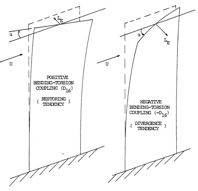
The physical mechanisms which cause this to be so are readily apparent in Fig. 3a and b. Figure 3a is a plate with a substantial positive D_{1 6}. In this case, aerodynamic

forces arising from plate displacements tend to return it to equilibrium, while just the opposite occurs with the plate having negative D_{1 6} (Fig. 3b).

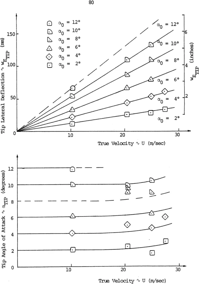
For the case where there is a known, nonzero, initial angle of attack, and a known dynamic pressure, the static deflections of the structure (a and w E) can be obtained by solving the equations of Eq. 2-41 simultaneously. For this study, only tip deflections are evaluated, because they were obtained experimentally.

U NEGATIVE BENDING-IORSION COUPLING (-D _{1 6} ) DIVERGENCE TENDENCY

Figure 3. Static Deflection Behavior

37

Eq. 2-41 can be rewritten as

kllql _{+ k} 1 2q2 = a 10 k 2lq1+ _{k22q2 = 2a0} where k = _{1 1}c k =2D _{1 6} 3C 12 X4 6 aa 3 k = 2D_{1 6} 21 V 6 4D k22 c66 18 + a = qct - I a2 a 2 D 11C2 48D 66' ll qe2 5 ~c 3 5

By solving Eqs. 2-45a and b following expressions for q

simultaneously, one obtains the

1 and q2'

(2-46a)

[

[k12k 2 1 - k1 1k 2 2]

(2-46b)

The generalized deflections are then transformed to actual deflections (ca and w E) using Eqs. 2-9 and 2-10, where $ and $ are evaluated at x = Z. As before, a

(2-45a)

(2-45b)

38

(Fig. 2b) equals the sum of a0 and a . The total angle of attack and bending deflection at the tip are

$a (x=Z) aTIP [ 1+ ( c aik₂.₁ - a₂k₁ k k - _{ak k 1 ) a} k12k21 1k k22 (2-47a) a_{2 k22} wE TIP _{k2l k21} aik2 -ak l1 k21 - k k2 k12 k21 k11 k22 )Ip₁(x=Z) a0 (2-47b)

2.5 Free Vibration Problem

The free vibration problem is formulated by setting the generalized forces (Q.) equal to zero in either Eqs. 2-25a and b, or Eqs. 2-29a, b and c. To make the equations of motion into algebraic equations instead of differential equations, one assumes that the motions of the plate will be harmonic. For harmonic (sinusoidal) motion, the gener-alized displacements can be expressed as

i = qeiot = 2 iWt

where w is the frequency. These expressions are substituted into the differential equations of motion (Eqs. 2-25 and 2-29) to obtain the sinusoidal equations of motion. The sinusoidal equations of motion are presented here, in matrix

39

form, for both the two term and three term deflection equations.

Two term deflection equation:

( 1 1 ) -w2 (mc I ) 2D_{1 6} 2 16) 2D

C161)

Three term deflection equation:

D C (-7) - W2(MroIg) (Il) w2 (eCI2 2D ₁₆ 29 £ ₂

q3

One obtains a unique solution to either Eq. 2-49 or

Eq. 2-50 by setting the determinant of the coefficient matrix equal to zero and solving for W2 (eigenvalue). The natural

2D 16, £26 2D 2D₁₆ 29

vibration frequencies (wn) are obtained by taking the square n

root of each eigenvalue. From Eq. 2-49, one obtains two natural frequencies (first bending and first torsion), and from Eq. 2-50, one obtains three natural frequencies (first bending, second bending and first torsion).

To simplify calculations, the warping stiffness term D _D11a2C

48D6 6z2

has been eliminated because its contribution is small for plates with moderate to high aspect ratios. The frequencies obtained using the mode shapes in Appendix B are compared in Chapter IV with experimentally obtained frequencies.

2.6 Aeroelastic Flutter Problem

The flutter problem is formulated using an indirect method widely known as the U-g method. In this method, the structural damping coefficient (g), introduced into the equations of motion, is plotted versus velocity for each vibration mode. Since solutions to the equations of motion represent conditions for neutral stability, the value of g obtained in this manner represents the amount of damping that must be added to the structure to attain

41

negative values of structural damping indicate that the

structure is stable. Flutter will occur when the artificial structural damping equals the actual damping of the structure. To simplify calculations, the flutter problem will be formu-lated using only the equations of motion from the two term deflection equation.

The equations of motion (Eqs. 2-24a and b), as derived in Section 2.2, again assuming sinusoidal motion and neg-lecting the warping stiffness contribution, are

-2

_[M.

j

Q₁ = f $lLE dx (2-52a) where LE c f2 pz dy Q Edx (2-52b) 0 C where ME c yz dy

Since aerodynamic forces and moments obtained by assuming steady flow are generally inadequate for realistic flutter calculations, complete unsteady aerodynamic expressions will be used. Unsteady aerodynamic lift (LE) and moment

(ME) expressions derived in Ref. 13 have been suitably trans-formed to the coordinate system in Fig. 2. The reader is cautioned that the coordinate system used throughout this study differs from the standard aeroelastic coordinate system used in Ref. 13. The difference being the +wE here is -h in Ref. 13. The aerodyanmic expressions are

LE = pb2 E + U - bad] _{+ 2pUbC (k) [-wE}

+ Ua + b(1/2 - a)& I (2-53a)

ME = rpb 3[-aME - U(l/2 - a)c - b(1/8 + a 2)d] +

7pUb 2(1/2 + a) C(k) [-wE + Ua + b(1/2 - a)& ]

43

where b = semichord

a = (distance EA is aft of midchord)/b _{(zero in} this study)

k = reduced frequency (ob/U) C(k) = Theodorsen function

Assuming sinusoidal motion

wE = iEwEe

E = -w wEeit

the aerodynamic expressions,

a. = eiWt

ai = loae

2raeir

after some algebraic manipu-lation, become LE = 2 rrpb 3{[ L₁ + iL2 -Eb b + [ L₃ + iL₄]a }eiWt (2-54a) where _{[ L + iL} 2 -2i W 1 k~ Ck L_{3 + iL} 4 W 2 pb4 2C(k) ]= _{a +- k2} + {[M + iM2 ] WE b t [ 1 + (1 - 2a) C(k)] + [ 3 + iM₄ ] a} e iot (2-54b) where M] = a - i (1+ 2a) C(k) M E

[ M₃ + iM ] = (1/8 + a ( ) + a2 v 2a 2(a) C (k)

+ [(1/2 - 2a 2) C (k) - (1/2 - a)]

Equations 2-54a and b are substituted into Eqs. 2-52a and b. One observes that, since the plate in this study has a con-stant chord, variables b, [ L + iL₂ ], [ L3 + iL₄ ],

[ M₁ + iM₂ ], and [ M3 + iM₄ ] are not functions of x and

can be brought outside the integral. Making use of the trans-formation equations (2-9 and 2-10), and expressing the integ-rals in nondimensional form, we arrive at the final expres-sions for the generalized forces.

313 L₁+ iL 2 Ql = 2 T 7 4

{

lpa

45

Substituting Eqs. 2-56a and b into Eq. 2-51 and can-celing eiot yields a new form of the equations of motion, which are written here in contracted matrix form.

K - w2A I j = 0 (2-56)

where the elements of

K _cD 1 1 7 2D₁₆ = I 12 £2 6 K 12 2D1 6 1 K21 2 6 4D6 6 22 c

a

the K.. and A.. matrices are given as

1J 1J A11 mckI₄ + 'pb2 4 [ L1 + iL2 Zb3 A₁₂ - 13 [ L3 + iL ] c A21 = _{£12 13 [ M + iM} 2 c mc + b 22 1 5 + p 2 5 3 +iM ₄ ] 12 c

Structural damping is proportional to, and opposes, the deflection of the structure. The structural damping coefficient (g) is introduced into Eq. 2-56 by multiplying the B matrix by (1 + ig). The methodology behind this step

is treated in depth in Ref. 13, An assumption here is that the linear damping coefficient (gh) is equal to the rotary damping coefficient (g ). It is also convenient to divide Eq. 2-56 by -w2 and combine it with the (1 + ig) term to

form a complex eigenvalue (Z), defined as

Z = ( ) (2-57)

Equation 2-53 now becomes

[ L - KZ ]g =0 (2-58)

where the elements of K are real and the elements of A are complex. The matrix [ A - KZ ] is put into standard eigen-value form by premultiplying by K , resulting in

[K 1 A - IZ ] = 0 (2-59) where I is an identity matrix, A unique solution to Eq.

2-59 is obtained by setting the determinant of the coeffi-cient matrix equal to zero, and solving for Z. For a 2 x 2 matrix, the two Z-values correspond to the two plate

vibra-tion modes (first bending and first torsion).

The solution procedure is to pick a value for the re-duced frequency (k) and solve Eq. 2-59 for Z.. The frequency structural damping coefficient and velocity are obtained

W = 1g = Im{Z} U = bw/k (2-60a,b,c)

/Re{ZT

Re{Z}

A new k value is chosen and the procedure is repeated.

Finally, a U-g diagram is created by plotting the structural damping for each root (Z) versus velocity, or a nondimensional

flutter speed (U/bw a), were wa is the torsional natural vib-ration frequency. One can get a reasonable approximation for W by picking a very large value for k and solving Eqs. 2-59 and 2-60a for the torsion root. This is essentially the structural vibration frequency when U equals zero. U-g diagrams for all the laminated plates considered in this study appear in Appendix B. The flutter velocity (UF) was conservatively chosen to be the point where the damping coefficient from either root first crosses the U-axis.

Solving the flutter problem is further complicated by the presence of the Theodorsen function (C (k)). The Theo-dorsen function is a nonrational functional which can be expressed exactly in terms of modified Bessel functions of the second kind. Since Eq. 2-59 was to be implemented on a digital computer and solved many times for different values of k, an approximation for C(k) was desired. By taking the Laplace Transform of R.T. Jones' exponential approximation, one obtains a rational expression for C(k). This expression is16

48 2 0,5.s2 + O.2808s + .0,01365 C(s) = -- (2-61) s2 + 0.3455s + 0.01365 where s is ik.

The flutter problem is now completely defined. For actual computation, taking the determinant of the 2 x 2 coefficient matrix is straightforward, the only complica-tions being that (1) the K-matrix must first be inverted and (2) that the coefficients of the A-matrix are all com-plex. Because of the simplicity of the problem, the temp-tation is to solve it manually. However, be advised that a typical U-g plot requires on the order of 20 data points. Each data point requires that Eq. 2-59 be solved for a new k value.

CHAPTER III EXPERIMENTS

3.1 Test Specimen Selection

Prior to making any test specimens, criteria which de-fined desirable, and sometimes essential, characteristics of the test specimens were established. These criteria in-cluded

(1) Test specimens must exhibit a wide range of bending-torsion coupling stiffness.

(2) Test specimens must be rectangular, constant thickness, flat plates with zero sweep. The requirement for a flat plate dictated using a symmetric laminate, since an unsymmetric laminate would warp during cure.

(3) Test specimens would be made from Hercules AS/3501-6 graphite/epoxy since it was available at M.I.T.

(4) Test specimens would have an aspect ratio of four, since this would be representative of an aircraft wing with an aspect ratio of eight.

(5) Test specimens should exhibit flutter and divergence within the 0 - 30 m/sec speed range of the acoustic wind tunnel at M.I.T.

(6) The test specimens should be small enought to be made using standard TELAC (Technology Laboratory for Ad-vanced Composites) ply cutting templates and curing

plates. Additionally, a small size was desirable be-cause the effect of slight material warping, often encountered during curing, would be minimized. (7) The laminate should be able to withstand repeated

large static and oscillatory loads.

Criteria five and six directly oppose one another when trying to arrive at an optimum design. Trying to satisfy both of them dictated a very thin plate. Also, to achieve substantial bending-torsion coupling, an unbalanced lamina-tion scheme was chosen. Unbalanced laminates have an unequal number of +e and

-e

to the limit results in a unidrectional laminate with all plies at +e or all plies at -0. To improve the toughness

(criterion seven) of a unidirectional, off-axis laminate, the center two plies would have a zero-degree ply angle. The total thickness was chosen to be six plies. Five different laminates were selected as representative of a wide range of bending-torsion coupling stiffnesses, both positive and negative. The first two laminates, [+302/0]s and [-302/03s' were chosen because a unidirectional laminate with

e

(D1 6) . The next two laminates, [+452/0]s and [-452/0 s'

were chosen because a unidirectional laminate with e = 45* exhibits the highest torsion stiffness (D6 6), but still has

a large D1 6. The final laminate, [02 /90s, was chosen

be-cause a unidirectional laminate with 8 = 00 exhibits the highest bending stiffness (D 1 1) and zero D1 6. During the

test program, another laminate, [*45/0]s , was added because it had the same theoretical D1 1 and D6 6 as [+4 52/0]s' with

less D_{1 6}. To minimize the number of test specimens which had to be constructed, the [+e2/0]s and [-e2/0]s test

spe-cimens were actually the same laminate, simply rotated

180 degrees about the x-axis (Fig. 1)

The test specimens would have to have an overall length of 330 mm (13 in) and a chord of 76 mm (3 in), be-cause this was the largest size that could be constructed satisfying criteria four and six. The overall length in-cluded a 25 mm (1 in) loading tab, making the effective cantilever plate length 305 mm (12 in). Finally, in an effort to minimize plate stiffness, an airfoil shaped fairing would not be used on the plate for wind tunnel tests. This had the added advantage of making the plate stiffness easier to calculate.

3.2 Test Specimen Preparation

The test specimens were constructed from Hercules AS/3501-6 graphite/epoxy prepreg tape from Lot No. 1643.

The tape was 305 mm (12 in) wide and had a nominal thick-ness of 0.134 mm (0.00528 in). Individual plies were cut

52

to the proper size and angular orientation using aluminum templates, and assembled into 305 mm (12 in) by 356 mm

(14 in) laminates. The laminates and curing materials (Ap-pendix C) were arranged on an aluminum curing plate especi-ally designed by students in TELAC for use with graphite/ epoxy laminates having a length and width as stated above. The laminates were cured in a Baron model BAC-35 autoclave using the cure cycle listed in Appendix C. After curing, the laminates were post-cured in a forced air circulation oven at 3504 F for eight hours. After post-curing, a rec-tangular test specimen 330 mm (13 in) long and 76 mm (3 in) wide was cut from each of the four laminates using a diamond

coated cutting wheel mounted on an automatic feed, milling machine.

The thickness of a graphite/epoxy plate tended to vary over its surface. Therefore, the plate thickness was measured at several different locations and averaged. The

same procedure was followed in measuring the length and width, although the variation was much less. The averaged measurements for each test specimen appear in Appendix D,

along with the nominal values. The thickness variation

between laminates (all were six ply) was 0.033 mm (0.0013 in) with the average being 0,807 mm (0.0318 in). This compared

favorably to the nominal thickness of 0.804 mm (0.0317 in) for a six ply laminate. The laminates were also weighed on a triple beam balance, from which the material density

53

(p)for each test specimen was calculated. The average den-sity was 1.53 x 103 kg/m3 (0.0554 lb/in 3) with a maximum variation of 0.06 x 103 kg/m3 (0.0022 lb/in 3). This again

compared favorably with a nominal density of 1.52 x 103 kg/m3 (0.055 lb/in _{3) for graphite epoxy.}

Loading tabs 83 mm (3.25 in) x 25.5 mm (1 in) were

machined from 2.4 mm (0.094 in) aluminum plate and bonded to the base of each test specimen with epoxy, cured at room

temperature. The loading tabs were intended to aid in align-ing the test specimen in the clampalign-ing fixture and to prevent damage to the plate surface fibers.

To get an indication of the lateral deflections the plate would experience during the wind tunnel tests, strain gauges were attached to the base of each test specimen at the midchord, as shown in Fig. 4. Two Micro Measurements EA-03-187BB-120 strain gauges, from Lot. No. R-A21AB02 with a gauge factor of 2.085, were attached to each test specimen

(one on each side) to measure bending strain, Two BLH-SR4; FAED-25B-12-59; Serial No. 5-AE-SC strain gauge rosettes from Lot No, A-315 with a gauge factor of 2.01 were attached to each test specimen (one on each side) to measure torsion strain. The two bending gauges were wired together as a

two-arm bridge circuit with three external lead wires approxi-mately 305 mm (12 in) long. The two torsion gauges were

wired together as a four-arm bridge circuit with four external lead wires. Wiring the strain gauges on either side of the

76.2 im (3")

H -

Sarrple Test Specinen

plate together, in this manner, doubled the signal output for each channel (bending and torsion) and provided auto-matic temperature compensation. This temperature

compen-sation was very important during the wind tunnel tests, where air flowing over an uncompensated gauge would cause a zero shift as the tunnel velocity was varied. The final step, after all solder connections had been made, was to coat the gauges with Micro Measurements M-Coat A, an air-drying poly-urethane, for protection.

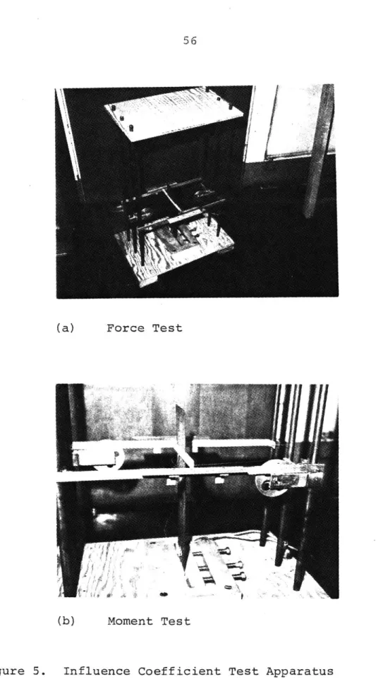
3.3 Test Apparatus and Procedure (a) Static Deflection Tests

The static deflection test setup is shown in Fig. 5. It consisted of a 330 mm (13 in) x 508 mm (20 in) plywood base with six vertical steel rods approximately 760 mm

(30 in) long. The test specimen was clamped in a vise machined from a 25.4 mm (1 in) x 152 mm (6 in) x 229 mm

(9 in) aluminum block, which was bolted to the base of the test fixture. Two removable, low friction, pulleys were attached to the vertical rods such that a force or moment could be applied to the test specimen at any location along its length. Rulers, graduated in 32nd's of an inch, were also attached to the vertical rods to facilitate measuring the test specimen's edge deflections. A deflection indicator

(a) Force Test

(b) Moment Test

57

was constructed out of balsa wood. It had needle pointers on the ends and cotton threads attached to its midpoint and ends. The threads, when routed over the pulleys and attached to weights, transferred a force or moment to the test speci-men (Fig. 5).

The deflection indicator was aligned with the lines scribed on the test specimen at the 3/4 length point, and the test specimen was clamped in the vise. The pulleys were clamped to the middle two vertical rods (Fig. 5a) at the proper height, and threads from the center of the deflec-tion indicator were routed over the pulleys. The rulers were adjusted to the proper height and zeroed with respect

to the deflection indicator pointers. Weights of 10, 20, 30, and 40 grams were successively attached to the threads, first to give positive deflections, then to give negative deflections. As each weight was attached, the readings from both pointers were recorded, along with the weight.

Next, the pulleys were moved to the corner rods (Fig. 5b) and the end threads were routed over them, so as to pro-vide a positive moment when the weights were attached. Weights of 10, 20, 33.9, and 43.9 grams were successively attached to each thread of the couple, and readings from both pointers were again recorded along with the weights. The pulleys were

then switched to the corner rods on the opposite diagonal, and theprocedure was repeated for a negative moment.

For each data point, the lateral deflection of the elastic axis (wE) and the rotation of the test specimen

about the elastic axis (a) were calculated using the data reduction formulas in Appendix E. The lateral deflections obtained from the load test (Test 1) were plotted versus

load, with the slope being the bending flexibility influence coefficient (c 1 1). The angular deflections (a) from Test 1

were plotted versus load, yielding the bending-torsion coupling flexibility influence coefficient (c2 1). The

an-gular deflections obtained from the moment test (Test 2) were plotted versus moment, yielding the torsion flexibility

influence coefficient (c2 2). The lateral deflections

ob-tained from Test 2 were plotted versus moment to obtain the other bending-torsion coupling flexibility influence coefficient (c1 2). The flexibility influence coefficient

plots for the four test specimens appear in Appendix E. The flexibility influence coefficients for a [+62 /0s and a [-82/0]s laminate will be the same, except for the sign on c1 2 and c21, since they were physically the same test

specimen. Finally, the flexibility influence coefficients for each test specimen were arranged in a 2 x 2 matrix (g)

and inverted to obtain the stiffness influence coefficient matrix (K). The results of the static deflection tests are

59

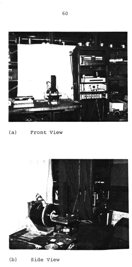
(b) Free Vibration Tests

The free vibration test setup, shown in Fig. 6, used the same vise as the static deflection tests. The vice was suspended by four spring steel strips, which allowed it to translate along the z-axis (Fig. 2), but restricted motion in all other directions. The vise was rigidly attached to a horizontally mounted Ling model 420 shaker using a cylin-drical aluminum adapter. The shaker had a peak force of 445 N (100 lbs) and a frequency range of approximately 5 to 3000 Hz. Since the shaker was driven by an audio amplifier, there was a certain amount of distortion to the sine wave output signal below 20 Hz. For some vibration tests, an Endevco model 7701-50 "Isoshear" accelerometer was mounted to the vise by a threaded mounting stud, and an Endevco model 222B "Micro-miniature" accelerometer was mounted to

the test specimen, within 25 mm of the base, using Eastman 910 adhesive. The outputs of these accelerometers, after passing through special amplifiers, were connected to a Tektronix type 502 dual beam oscilloscope so that both out-puts could be displayed simultaneously. Finally, a digital signal counter was attached directly to the signal generator to provide an accurate frequency readout.

The test specimen was aligned and clamped in the vise. A white paper screen was suspended behind the test specimen

(a) Front View

(b) Side View