HAL Id: tel-02294630
https://tel.archives-ouvertes.fr/tel-02294630
Submitted on 23 Sep 2019HAL is a multi-disciplinary open access archive for the deposit and dissemination of sci-entific research documents, whether they are pub-lished or not. The documents may come from teaching and research institutions in France or abroad, or from public or private research centers.
L’archive ouverte pluridisciplinaire HAL, est destinée au dépôt et à la diffusion de documents scientifiques de niveau recherche, publiés ou non, émanant des établissements d’enseignement et de recherche français ou étrangers, des laboratoires publics ou privés.
Exploring the determinants of household electricity
demand in Vietnam in the period 2012–16
Hoai-Son Nguyen
To cite this version:
Hoai-Son Nguyen. Exploring the determinants of household electricity demand in Vietnam in the period 2012–16. Economics and Finance. Université Paris Saclay (COmUE), 2019. English. �NNT : 2019SACLA013�. �tel-02294630�
Exploring the determinants of
household electricity demand in
Vietnam in the period 2012 16
Thèse de doctorat de l'Université Paris-Saclay préparée à AgroParisTech (l'Institut des sciences et industries du vivant et de l'environnement) École doctorale n°581 ABIES Spécialité de doctorat: sciences économiquesThèse présentée et soutenue à Paris, le 24 Juin 2019, par
Hoai-Son NGUYEN
Composition du Jury : M. Phu NGUYEN VAN
Directeur de Recherche, (BETA & Université de Strasbourg) Président M. Michel SIMIONI
Directeur de Recherche, (INRA) Rapporteur
M. Joachim SCHLEICH
Professeur (Grenoble École de Management) Rapporteur M. Phu LE VIET
Lecturer ( Fullbright University, Vietnam) Examinateur Mme Carine BARBIER
Ingénieure de Recherche (CIRED) Examinateur
M. Minh HA DUONG
Directeur de Recherche (CIRED) Directeur de thèse
N N T : 20 19 S A C LA 0 13
ACKNOWLEDGEMENT
First of all, I would like to convey my grateful attitude and great appreciation to my supervisor, Dr. Minh HA-DUONG for granting me the chance to conduct this thesis. He not only offers financial funding for my thesis but also shows his profound belief in my abilities and encourages me to explore my best capacity. He consistently allowed the thesis to be my own work but steered me in the right the direction whenever he thought I needed it. It was very especial that he also provided me with the best place for thesis writing that I can imagine, as major part of my thesis was written in his house in Bagneux, next to a wood-burning stove. I am extremely grateful to my jury and thesis committee, Dr. Phu NGUYEN-VAN, Dr. Michel SIMIONI, Dr. Joachim SCHLEICH, Mme. Carine BARBIER, Dr. Phu LE-VIET and Dr. Gilles CRAGUE. I am deeply indebted to them for their insightful comments and tough questions, which realized my thesis. I would particularly like to thank Mrs. Elisabeth MALTESE, my French teacher, for her patience and kindness, so that I was able to complete my French course as a required condition for my thesis submission.
I would like to sincerely thank Mrs. Marguerite CZARNECKI for translating the thesis summary to French and Mrs. Pippa CARRON for copyediting the first draft of the thesis. They both performed their works at the light speed to help me submit my thesis in time. I also gratefully acknowledge the assistance of the lecturers, colleagues and staffs at CIRED and ABIES.
My heartfelt appreciation goes to my best friend Hoang Anh and his family who always there encouraging me and make Paris my second home whenever I am in Paris.
The thesis would not have been possible without the great support and motivation I get from my wife, Nha Trang and my little two angels, Lam Bach and Khai An. And my special thanks go to my parents-in-law for helping us with our boys when I was away from Viet Nam for the thesis.
Last but not least, this thesis is dedicated to my beloved father Mr. Ban NGUYEN-VAN and mother Mrs. Lan LE-NGOC for the great and small things they have done for me.
1
Contents
Chapter 1. Introduction ... 6
Chapter 2. Background information and policy context ... 8
2.1 Overview of the residential electricity market ... 8
2.2 Residential electricity prices ... 8
2.3 Subsidy in residential electricity ... 9
2.3.1 Subsidy in electricity prices ... 9
2.3.2 Subsidy in cash transfer for poor households ... 10
Chapter 3. Model specification ... 11
3.1 Short-run versus long-run demand functions ... 11
3.1.1 Theory models of electricity demand function ... 11
3.1.2 Empirical models for electricity demand estimation ... 14
3.2 Model specification ... 20
Chapter 4. Data ... 22
4.1 Temperature data ... 22
4.2 Vietnam Household Living Standard Survey data... 23
4.2.1 Overview of VHLSS ... 23
4.2.2 VHLSS samples ... 24
4.2.3 Sample rotation, survey time and weight ... 26
4.2.4 Data process from VHLSS ... 26
4.3 Merging electricity price with VHLSS ... 27
4.4 Merging temperature data with VHLSS ... 28
4.5 Deflating monetary variables to a base year and cleaning data ... 29
4.6 Data sets for short-run and long-run demand function ... 29
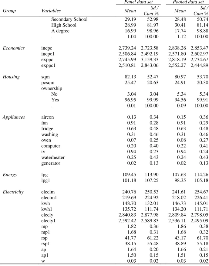
4.7 Descriptive statistics ... 30
Chapter 5. Price elasticity of residential electricity demand ... 33
5.1 Introduction ... 33
5.2 Literature review ... 33
5.2.1 Controversy in the type of prices ... 33
5.2.2 Models for testing price types ... 36
5.2.3 Endogeneity in block pricing ... 38
5.3 Model specification and data ... 39
5.3.1 Short-run model ... 39
5.3.2 Long-run model ... 42
5.3.3 Perceived price model ... 42
5.3.4 Econometric techniques ... 42
5.3.5 Data ... 44
5.4 Results and discussion ... 44
5.4.1 Short-run demand ... 44
5.4.2 Long-run demand ... 54
5.4.3 Perceived price model ... 58
5.5 Conclusion ... 59
Chapter 6. Income and electricity poverty in Vietnam 2012–16 ... 61
6.1 Introduction ... 61
6.2 Literature review ... 61
6.2.1 Direct measurement approach ... 62
6.2.2 Indirect measurement approach ... 62
6.3 Methods and data ... 64
6.4 Results ... 66
2
6.4.2 Econometric approach ... 67
6.5 Conclusion ... 69
Chapter 7. Economies of scale in residential electricity consumption ... 71
7.1 Introduction ... 71
7.2 Literature review ... 71
7.2.1 Economies of scale ... 71
7.2.2 Economies of scale for household electricity expenditure ... 72
7.3 Methods and data ... 74
7.3.1 Non-parametric method ... 74
7.3.2 Parametric method ... 76
7.3.3 Data ... 78
7.4 Results and discussion ... 79
7.4.1 Non-parametric analysis ... 79
7.4.2 Parametric analysis ... 81
7.5 Conclusion ... 83
Chapter 8. Heatwaves and residential electricity demand... 85
8.1 Introduction ... 85
8.2 Literature review ... 85
8.3 Methods and data ... 87
8.3.1 Methods ... 87
8.3.2 Data ... 88
8.4 Results and discussion ... 89
8.5 Conclusion ... 91
3
List of tables
Table 2-1. The three most recent retail electricity prices for residential ... 9
Table 2-2. Evolution of electricity subsidy in cash transfer ... 10
Table 3-1. Electric appliances in different research papers ... 17
Table 4-1. List of weather stations in GHCN data ... 22
Table 4-2. Available data on each round of VHLSS 2008–16 ... 24
Table 4-3. Sample sizes of VHLSS from 2008–2014 ... 25
Table 4-4. Number of wards/EA in each round of VHLSS ... 25
Table 4-5. Number of households selected in each EA ... 25
Table 4-6. Survey plan for VHLSS 2008–2014 ... 26
Table 4-7. Paired t-test for mean comparison between original and calculated kWh ... 27
Table 4-8. Similarity between data sets for short-run and long-run function... 31
Table 4-9. Differences between data sets for short-run and long-run functions ... 32
Table 5-1. Income per capita at 2012 price over dwelling type ... 40
Table 5-2. Pairwise comparison of income per capita at 2012 price over dwelling type ... 40
Table 5-3. Estimated results of the short-run demand function ... 46
Table 5-4. Endogeneity tests for the short-run demand function ... 46
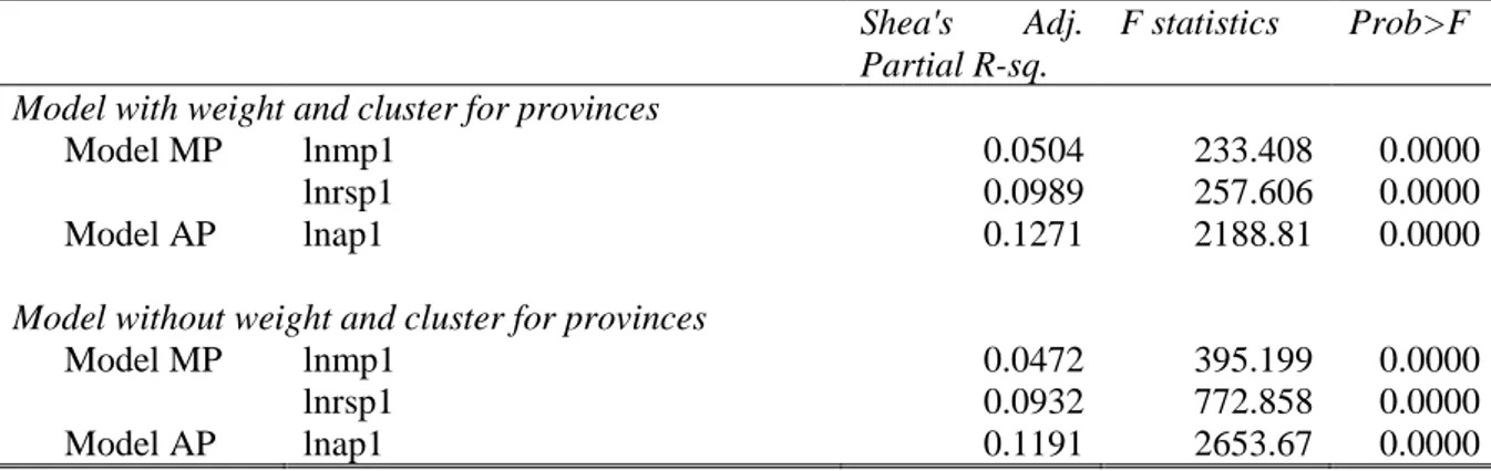
Table 5-5. Weak instrument tests for the short-run demand function ... 47
Table 5-6. Pairwise correlation between prices and price IVs ... 48
Table 5-7. Weak instrument tests from first stage regression for the short-run function ... 48
Table 5-8. Sensitivity analysis for different sub-samples... 49
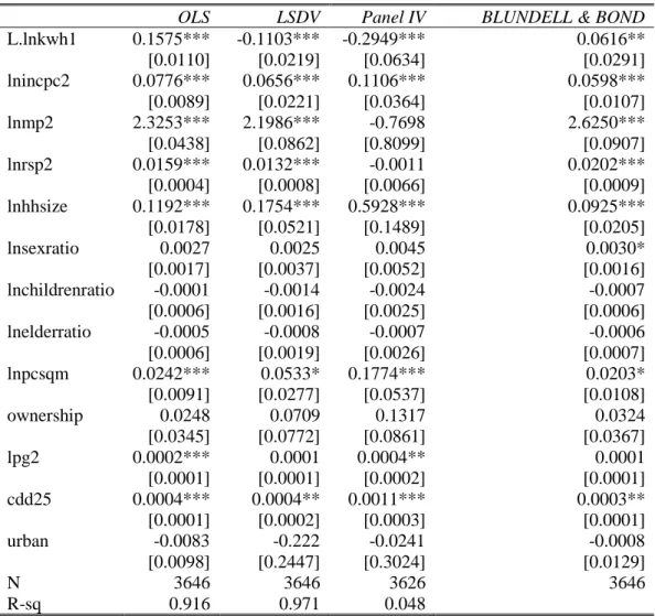
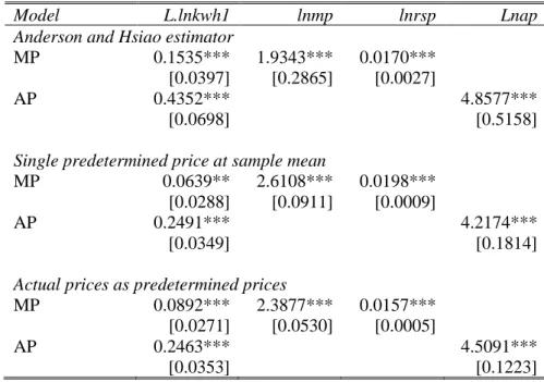
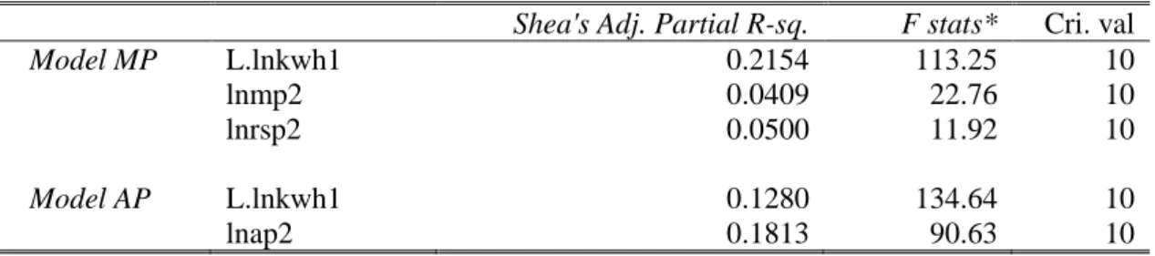
Table 5-9. Estimated long-run function of MP model ... 55
Table 5-10. Estimated long-run function of MP model ... 56
Table 5-11. Robustness tests for the long-run model with different IVs and estimators ... 56
Table 5-12. Endogeneity tests for long-run models ... 57
Table 5-13. Weak instrument tests for long-run models ... 57
Table 5-14. Short-run estimates with the panel as a pooled data ... 58
Table 5-15. Estimates for perceived price model ... 59
Table 6-1. Estimates of kWh per cap on the quantiles of income per cap ... 68
Table 6-2. Average kWh consumption of households having corresponding income quantiles ... 69
Table 6-3. Electricity services a household can consume with 50 kWh per month ... 69
Table 7-1. Correlation between income and demographic variables. ... 77
Table 7-2. Household types and household groups for non-parametric analysis ... 78
Table 7-3. The average electricity share weighted by the density of income per capita ... 80
Table 7-4. Estimation of parametric approach for economies of scale in electricity expense . 82 Table 7-5. Sensitivity analysis for economies of scale in electricity expense ... 82
Table 8-1. Descriptive of heatwave dummy variable ... 89
4
List of figures
Figure 2-1. Increase in electricity demand, 2006–2015 (Unit. KTOE) ... 8
Figure 4-1. Position of the 14 weather stations ... 23
Figure 4-2. Rotation for VHLSS sampling ... 26
Figure 4-3. The construction of data sets for short-run and long-run functions ... 30
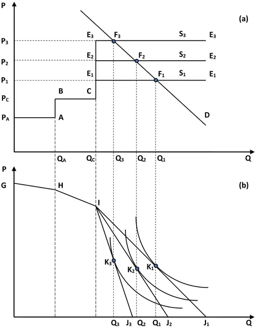
Figure 5-1. Changes of marginal price and demand ... 34
Figure 5-2. Changes of intra-marginal price and demand ... 35
Figure 5-3. Scatter density plot with fitted line for prices and price IVs ... 47
Figure 6-1. The S-shaped relationship between household income and kWh consumption .... 64
Figure 6-2. Density scatter plots with a series of fitted lines for different income quantiles ... 67
Figure 7-1. Channels of economies of scale in household electricity expenditure ... 74
Figure 7-2. Illustration of wm and f(zm) over regression grid ... 76
Figure 7-3. Non-parametric analysis for economies of scale ... 79
5
Abbreviations list
AC Air conditioning
AP average prices
CDD cooling degree days CPI consumer price index
CSCTWA cross-sectionally correlated and time-wise autoregressive model CSHTWA cross-sectionally heteroscedastic and time-wise autoregressive model DBT decreasing block tariff
EA enumeration area ECM error correction model EOS economies of scale EVN Vietnam Electricity
GADM Global Administrative Areas
GHCN Global Historical Climatology Network GMM generalized method of moments
HDD heating degree days IBT increasing block tariffs IVs instrument variables kWh kiloWatt hour
LB lower bound
LkWh lower bound kWh LPG liquefied petroleum gas LSDV least square dummy variables MoF Ministry of Finance
MoIT Ministry of Industry and Trade
MP marginal prices
MPHS Multi-Purpose Household Survey
NOAA National Oceanic and Atmospheric Administration (US) NOOA National Centers for Environmental Information
OLS ordinary least squares
PPS probability proportionate to size (rule of) PSU Primary sample unit
RSP rate structure premium SSU Secondary sample unit TSU Tertiary sample unit TVs televisions
UB upper bound
UkWh upper bound kWh UHI urban heat island VAR vector autoregressive
VHLSS Vietnam Household Living Standard Surveys VLSS Vietnam Living Standard Survey
VND Vietnamdong
6
Chapter 1. Introduction
In recent years, demand-side management in residential electricity markets has been a major tool for developing countries in harmonizing economic growth, energy security, and reduction of CO2 emissions.
First, demand-side management tools, such as increasing block-tariff schedules have potential in encouraging people to save electricity, which in turn reduces carbon emissions from electricity generation associated with fossil fuel consumption. This is important for Asian countries where a large proportion of electricity supply is still based on coal. Developing countries, particularly in Southeast Asia, use coal to ensure continuity of supply.
Second, demand-side management also helps developing countries ensure energy security by constraining the surging demand in electricity. Developing countries face higher tension in electricity markets than developed countries. In developed countries, the market is well established, and demand is relatively stable. Supply sources in those countries can gradually transition to a structure with a higher proportion of renewable sources while providing for economic growth. In developing countries, the market is growing fast, and demand soars due to economic growth and rapid population increase. The fast-rising demand surpasses electricity supply capacity causing power outages. Demand-side management can constrain the fast-rising demand to be in line with current supply capacity.
Demand-side management implementation in residential electricity markets requires a deep understanding of customer behaviors, and household demand. In the past, much has been done with aggregate data to explore factors impacting on residential electricity demand (Houthakker, Verleger and Sheehan, 1974; Hsing, 1994; Holtedahl and Joutz, 2004; Alberini and Filippini, 2011). However, recently two points have emerged that set new challenges in estimating electricity demand. First, there is a movement from aggregate data to micro data at a household level, but the micro data is often either missing data in price (Branch, 1993; Alberini, Gans and Velez-Lopez, 2011) or is narrowed to a regional level rather than a national level due to the absence of national data on tariff structures (Reiss and White, 2005; Zhou and Teng, 2013). Second, climate change has recently introduced a new factor of heatwaves which has not been carefully investigated in electricity demand in the past.
Therefore, this thesis revisits the story of electricity demand estimation within the context of Vietnam over the period 2012–16. Four reasons justify this context. First, Vietnam is a tropical country with frequent summer heatwaves so is ideal for investigation of the impact of heatwaves on electricity demand. Second, the micro survey in Vietnam is a rotated survey which allows the construction of a panel data set from three rounds in three different years, as well as the construction of a pooled data set from the rest. The separation of data into panel and pooled data is ideal to estimate electricity demand both in short-run and long-run. Third, the residential electricity market in Vietnam is a monopoly with a single seller, Vietnam Electricity (EVN). Electricity tariff schedules are proposed by EVN and set by the government and are thus uniform in national scale. This provides a chance to estimate demand function from national micro survey data with full detail of electricity prices.
Finally, Vietnam is a country carrying full features of a developing country, with increasing role of demand-side management. Due to the rapid pace of economic growth, electricity demand in Vietnam has surged, causing challenges in ensuring energy security as well as in developing renewable energy sources. During the period from 2006 to 2015, national electricity consumption grew at an average rate higher than 10 per cent (MOIT and DEA, 2017). Demand for electricity by 2035 is predicted to grow at an average annual rate of eight per cent (MOIT
7 and DEA, 2017). Almost half of the new capacity is proposed to be coal fired (MOIT and DEA, 2017). In response to this issue, the Vietnamese government considers energy efficiency as a “first fuel”. Electricity saving is estimated potentially at 17 per cent by 2030 (MOIT and DEA, 2017). In practice, the government has implemented measures such as increasing the block tariff schedule for residential consumption to encourage people to save electricity (EVN, 2015). In that context, the results of this thesis not only broaden our understanding of residential electricity demand functions in developing countries, but also provides a reference for policy makers in designing measures to manage demand side in Vietnam.
This thesis aims to explore the factors which impact on Vietnamese residential electricity demand. The exploration focuses on four main factors: increasing block tariffs, income, demographics (including household size and composition), and heatwaves. The approach is to investigate the role of these factors via estimating a common form of demand function, with each factor investigated in detail in separate chapters.
The master data for this thesis are constructed from Vietnam Household Living Standard Surveys (VHLSS) 2012, 2014 and 2016, various legal documents on electricity prices, and temperature data from the National Centers for Environmental Information (NOOA) over the corresponding period. The period of 2012–16 was chosen because (i) 2016 is the most updated data we have so far and (ii) the rotated features of VHLSS allows the construction of panel data with a maximum of three rounds. The master data are then separated into two sub-datasets: (i) panel data, including households that appear in all three years; and (ii) pooled data, including households that appear only once in all three years. The two sub-datasets are employed to estimate short-run and long-run demand functions.
The thesis is structured as follows. Chapter 2 provides a policy context and some background information on the Vietnam electricity market. Chapter 3 provides a general literature review which details the theory models and empirical strategy for short-run and long-run functions of electricity demand. Chapter 4 provides detail about the procedure of constructing data sets. Chapter 5 focuses on increasing block tariffs and examines the impact of increasing the block tariff schedule on residential demand. The two aims of the chapter are: (i) to estimate the price elasticity of demand in short-run and long-run; and (ii) to identify whether households respond to marginal prices or average prices.
Chapter 6 focuses on income. It investigates the non-linear relationship between income and electricity demand and its implication for identifying the electricity poverty threshold. The hypothesis is the existence of an income threshold whereby electricity consumption starts to increase with an increase in income. The consumed kWh per capita of households at that income threshold is the electricity poverty threshold.
Chapter 7 focuses on the role of two demographic factors: household size and household composition. The chapter answers two questions: (i) whether the increasing block tariff schedule cancels out the economies of scale in electricity use in Vietnam; and (ii) whether there is a difference in electricity demand across a child, an adult and an elder in Vietnam.
Chapter 8 focuses on the impacts of heatwaves on household electricity demand. The chapter aims to demonstrate that cooling degree days (CDD) – a popular way to represent temperature in electricity demand function – is insufficient to capture the full impact of temperature since it neglects the extreme distribution of temperature which are heatwaves in tropical countries.
8
Chapter 2. Background information and policy context
2.1 Overview of the residential electricity market
❖ The surging demand
Due to the rapid pace of economic growth, electricity demand in Vietnam has surged in recent years. During the period from 2006 to 2015, national electricity consumption grew at an average rate higher than 10 per cent (MOIT and DEA, 2017). The demand for electricity by 2035 is predicted to grow at an average annual rate of eight percent (MOIT and DEA, 2017).
Figure 2-1. Increase in electricity demand, 2006–2015 (Unit. KTOE) Source. MOIT and DEA (2017, p. 16).
Residential consumption plays a vital role in the sharp increase in electricity demand. First, residential demand accounts for a large proportion of total electricity demand. For example, the total electricity consumption of households accounted for 54 per cent of total electricity consumption in Ha Noi in 2018 (Tiến Hiệp, 2018). Second, the rate of access to electricity of households is 98 per cent (authors calculated from VHLSS 2012–16). With economic growth, households have increased wealth and more electrical appliances resulting in a higher demand for electricity.
❖ Monopoly in residential electricity market
Since 2004, several legal documents have been aimed at removing the monopoly in electricity markets, including the residential electricity market. The electricity law (2004) and Decision 26 (2006) regulated that: (i) government is the monopoly in transmission; (ii) generation would be competitive by 2014; (iii) wholesale distribution would be competitive by 2022; and (iv) retail distribution would be competitive from 2022. In 2013, Decision 63 (2013) adjusted the plan to have pilot competitive wholesale in 2015 and officially competitive wholesale in 2021. In reality, the implementation of the roadmap lags behind the plan. The generation market started to operate in July 2012 with a short suspension in 2017. The competitive wholesale distribution market started to operate in January 2019. Basically, the residential electricity market up to 2019 was a monopoly with Vietnam Electricity (EVN) as a single seller.
2.2 Residential electricity prices
Residential electricity prices in Vietnam are set by the government under Decision 69 of 2013 (Nguyễn Tấn Dũng, 2013). According to the decision, the price schedule is set based on an average electricity selling price. The average electricity selling price is calculated from the production costs and a reasonable level of profit at four stages, including generation, transmission, distribution and supporting services. When the basic input parameters change,
9 EVN recalculates the average electricity selling price and submits it to the government for approval. The basic input parameters are factors that have a direct impact on the cost of generating electricity that are out of the control of the generating units, including fuel prices, foreign exchange rates, and structure of the actual electricity generation, as well as prices in competitive electricity generation markets.
Residential electricity prices in Vietnam have been in the form of increasing block tariffs (IBTs) since 1994. The IBTs mean that the higher kWh a household consumes, the higher the price per kWh. Households pay a low price for the first block, then pay a higher price for a second block, and so on. According to EVN (2015), IBTs aim to encourage a savings attitude and ensure a low price for low-income households.
Block Lower bound Upper bound Apr 2015 – Nov 2017 Dec 2017 – Feb 2019 Mar 2019 – present 1 1 50 1,484 1,549 1,678 2 51 100 1,533 1,600 1,734 3 101 200 1,786 1,858 2,014 4 201 300 2,242 2,340 2,536 5 301 400 2,503 2,615 2,834 6 401 2,587 2,701 2,927 ASP 1,622.01 1,720.65 1,864.44
Note. Unit ‘000 Vietnamdong per kWh; ASP: average selling price; VAT excluded. Unit for lower bound and upper bound is kWh per month.
Table 2-1. The three most recent retail electricity prices for residential Source. Author compiled from various legal documents.
There are two price schedules of prices for residential electricity in Vietnam. Both schedules are in IBTs form. The first is the retail price schedule which applies to households that can buy electricity directly from EVN. The second is for wholesale prices. Wholesale prices are applied to rural areas which are remote, have low population density and unorganized infrastructure. In these areas, EVN sells electricity to rural electricity distribution organizations with the wholesale price schedule. These organizations sell electricity to households with their own price schedule based on the wholesale prices. There is heterogeneity in price setting of these organizations. Some apply a single price, while others may apply a three-block design, and so on.
However, the wholesale price schedule is applied only to a small fraction of households. In 2014, EVN provided electricity directly to 84.57 per cent of communes, and 82.59 per cent of rural households (Thục Quyên, 2014). In 2015, EVN provided electricity directly to 87.88 per cent of rural households in Southern provinces (Mai Phương, 2015).
2.3 Subsidy in residential electricity 2.3.1 Subsidy in electricity prices
Poor or low-income households which (i) have monthly electricity consumption less than 50 kWh and (ii) register with EVN can have a special price for the first 50 kWh. The prices for the special block are about 80 per cent of the approved average selling price in 2011, then gradually decreased to 65 per cent in the period from August 2013 to May 2014. Meanwhile, the prices for the normal first block (0–100 kWh) is normally equivalent to 95 per cent of average selling prices. However, since June 2014, the subsidy block has been canceled.
10 For other households, during the period from March 2011 to May 2014, the first block was from 0 to 100 kWh. The price of the first block is about 95% of average selling price. However, since June 2014, the first block has been divided into 2 blocks. Block 1 is from 0 to 50 kWh. Block 2 is from 51 to 100 kWh. The price of Block 2 is three percentage points higher than the price of Block 1 in term of percentage to average selling price.
2.3.2 Subsidy in cash transfer for poor households
Since 2011, in parallel to the subsidy in electricity prices, the Vietnamese government has also implemented an electricity subsidy program of cash transfers for poor households. According to the program, every household under the national poverty line can receive 30,000 VND (about USD 1.5) each month (Nguyễn Tấn Dũng, 2011). The subsidy is in cash every quarter (Nguyễn Công Nghiệp, 2012).
Periods Subsidy Beneficial kWh Cash
Dec 2011 to
May 2014 30,000
- Poor households
• Rural: 400,000 VND per cap per month • Urban: 500,000 VND per cap per month
Jun 2014 to
May 2015 30 46,000 - Poor households: national poverty line, if provinces have their own line higher than national line, then apply the province line. • Rural: 700,000 VND per cap per month
• Urban: 900,000 VND per cap per month - Households under preferential treatment policy Jun 2015 to Nov 2017 30 49,000 Dec 2017 to present 30 51,000
Note. Unit: Vietnamdong.
Table 2-2. Evolution of electricity subsidy in cash transfer Source. Author compiled from various legal documents.
In 2014, the subsidy amount was set to 30 kWh at prevailing prices (Đỗ Hoàng Anh Tuấn, 2015). In 2014 prices, the 30 kWh costs 46,000 VND (about USD 2.0). In addition, the benefit is extended to include households under the preferential treatment policy (Nguyễn Tấn Dũng, 2014b). The extended beneficiaries are: (i) non-poor households with members receiving monthly social allowance and consume less than 50 kWh per month from the national grid for living purposes; (ii) households with members receiving the monthly social allowance living in a non-grid area; and (iii) ethnic minority households living in a non-grid area.
In June 2015, due to an increase in electricity price, the subsidy increased to 49,000 VND (Nguyễn Tấn Dũng, 2015). At the new price in December 2017, the subsidy increased to 51,000 VND. In July 2018, the Ministry of Finance (MoF) submitted a proposal cancelling the cash transfer program (H.Anh, 2018). The proposal faced a backlash and so in October 2018 the MoF submitted a draft circular that kept the cash transfer subsidy program at the threshold of 30 kWh (Bộ Tài Chính, 2018).
11
Chapter 3. Model specification
3.1 Short-run versus long-run demand functions
This study focuses on the residential electricity demand function. Unlike other commodities consumed by households, electricity by itself does not generate utility for consumers. The use of electricity needs to go with appliances such as fans, air conditioners (AC) and televisions (TV). Thus electricity demand can be considered as a derived demand which depends on demand of appliances in households (Taylor, 1975).
Since electricity demand depends on the availability of appliances, there are two types of demand function: short-run and long-run. A short-run demand function is defined by a condition that the appliance stock is fixed (Taylor, 1975, p. 80), while in the long-run function the appliance stock can vary (Taylor, 1975, p. 80).
3.1.1 Theory models of electricity demand function
Fisher and Kaysen (1962) was the first study to explicitly distinguish between short-run and long-run electricity demand functions. Houthakker and Taylor (1970), based on the idea of capital stock in Fisher and Kaysen, derived a complete model for residential electricity demand in both short-run and long-run. So far, most models in electricity demand at the household level are constructed based on the ideas of these two models. The following parts provide a brief explanation of the two models.
3.1.1.1 Fisher and Kaysen (1962)
Fisher and Kaysen (1962) is the pioneer research which distinguished between short-run and long-run demand functions. Fisher and Kaysen (1962) assert that short-run demand is the utilization of appliance which they describe using the term “white goods”.
❖ Short-run function
The total electricity consumption of a household (D) during period t is the additive function of electricity consumption of n appliances. The electricity consumption of an appliance, in turn, is the product of its intensity use (K) with the average stock of the appliance (W). The average stock is measured by the kWh that the appliance consumes in an hour of normal use.
𝐷𝑡 = ∑𝑛𝑖=1𝐾𝑖𝑡𝑊𝑖𝑡 (3-1)
The intensity of use of the ith appliance is a function of electricity price (P) and income (Y) 𝐾𝑖𝑡 = 𝐵𝑖𝑃𝑡𝛼𝑖𝑌 𝑡 𝛽𝑖 (3-2) Substitute (3-2) to (3-1), we have 𝐷𝑡 = ∑ 𝐵𝑖𝑃𝑡 𝛼𝑖𝑌 𝑡 𝛽𝑖𝑊 𝑖𝑡 𝑛 𝑖=1 (3-3)
They then define 𝐶𝑖 = 𝐵𝑖𝑃̅𝑡
𝛼𝑖𝑌̅
𝑡
𝛽𝑖 (3-4)
𝑃̅ and 𝑌̅ are the mean of 𝑃𝑡 and 𝑌𝑡 over T times period. So the (3-4) becomes 𝐷𝑡 = ∑ 𝐶𝑖(𝑃𝑡/𝑃̅)𝛼𝑖(𝑌
𝑡/𝑌̅)𝛽𝑖𝑊𝑖𝑡 𝑛
12 Fisher and Kaysen assume that (3-5) can be approximated by (3-6) with C, α, β being constant.
𝐷𝑡 = 𝐶(𝑃𝑡/𝑃̅)𝛼(𝑌𝑡/𝑌̅)𝛽∑𝑛𝑖=1𝑊𝑖𝑡 (3-6)
Taking logarithms of both sides of (3-6)
𝑙𝑛𝐷𝑡 = 𝐶0+ 𝛼𝑙𝑛𝑃𝑡+ 𝛽𝑙𝑛𝑌𝑡+ 𝑙𝑛𝑊𝑡∗ (3-7) Where 𝐶0 = 𝑙𝑛𝐶 − 𝛼𝑙𝑛𝑃̅ − 𝛽𝑙𝑛𝑌̅ (3-8) 𝑊𝑡∗ = ∑ 𝑊 𝑖𝑡 𝑛 𝑖=1 (3-9)
𝑊𝑡∗ is the stock of all appliances.
Now the short-run demand function would be
𝑙𝑛𝐷𝑡− 𝑙𝑛𝑊𝑡∗ = 𝐶0+ 𝛼𝑙𝑛𝑃𝑡+ 𝛽𝑙𝑛𝑌𝑡 (3-10)
Where α and β are the price and income elasticities at the period t. ❖ Long-run function
Once white goods are measured by the amount electricity they consume, the long-run demand of electricity is equivalent to the demand for white goods at each household. Thus Fisher and Kaysen (1962) construct a model to explain the changes of household demand for white goods. The key assumption of the model is that the changes are not proportional to the difference between the actual and desired stock of appliances. Fisher and Kaysen argue that for heavy electricity load appliances, each household normally own just one unit. The change of appliance stock at aggregate level is due to the new consumption of households who have not owned these appliances before. Thus the proportion of actual stock is meaningless since actual current stock is zero. In addition, the proportion at the aggregate level includes irrelevant households who have already owned appliances before.
Thus Fisher and Kaysen (1962) propose a model in which the change of white good stocks from time t-1 to time t depends on the changes of permanent income, current income, price of electricity and gas, price of both electricity appliances and gas-using competitors, and other demographic variables. The model is as follows:
∆𝑙𝑛𝑊𝑖𝑡 = 𝐴𝑖 + 𝛾𝑖1∆𝑙𝑛𝑌𝑡𝐸+ 𝛾 𝑖2𝑙𝑛𝑌𝑡+ 𝛾𝑖3𝐸𝑖𝑡+ (𝛾𝑖4𝑙𝑛𝐺𝑖𝑡) + 𝛾𝑖5∆𝑙𝑛𝐻𝑡+ 𝛾𝑖6∆𝑙𝑛𝐹𝑡+ 𝛾𝑖7𝑙𝑛𝑀𝑡+ 𝛾𝑖8𝑙𝑛𝑃𝑡𝐸 + (𝛾 𝑖9𝑙𝑛𝑉𝑖𝐸) + 𝑢𝑖𝑡 (3-11) where 𝑊𝑖 = stock of appliance i
𝑌𝐸 = Friedman permanent income Y = current per capita income 𝐸𝑖 = price of appliance
𝐺𝑖 = price of gas-using competitor
H = number of urban residential over population F = number of marriages
𝑃𝐸 = 3-year moving average of electricity price 𝑉𝐸 = 3-year moving average of gas price
13
3.1.1.2 Houthakker and Taylor (1970)
Houthakker and Taylor (1970) also use the definition of Fisher and Kaysen (1962) on white good stocks which are measured by the amount of Watt that the appliance can draw. Houthakker and Taylor (1970) develop two separate models for short-run and long-run based on utility theory as follows.
❖ Short-run function
Houthakker and Taylor consider demand as the utilization of capital stock. The utility is a function of price, income and other factors as set out below.
𝑞 = 𝑢(𝑥, π, z)s (3-12)
where
u(.) = utility function x = income
π = price
z = other factors
s = the stock of appliance is measured by the amount of Watt that the appliances can draw as defined in Fisher and Kaysen (1962).
Let 𝑢 = 𝛼0+ 𝛼1𝑥 + 𝛼2𝜋 + 𝛼3𝑧 (3-13)
The short-run demand (3-12) turn to
𝑞 = (𝛼0+ 𝛼1𝑥 + 𝛼2𝜋 + 𝛼3𝑧)𝑠 (3-14)
In short-run, the impact of price and income on electricity demand is 𝜕𝑞
𝜕𝑥 = 𝛼1𝑠 (3-15)
𝜕𝑞
𝜕𝜋= 𝛼2𝑠 (3-16)
❖ Long-run function
The long-run model is derived from a state adjustment model developed by Houthakker and Taylor (1970). The name “state” adjustment model comes from the assumption that flows respond to the difference between actual and desired states.
In long-run, the expenditure flow on appliance stock is a function of the level of appliance stocks (state variables), income flows and the level of prices which can vary over time.
𝐸(𝑡) = 𝛼 + 𝛽𝑠(𝑡) + 𝛾𝑥(𝑡) + 𝜃𝑝(𝑡) (3-17)
where
E(t) = expenditure flows on new appliance during a very short time interval around t s(t) = a state variable stands for appliance stock at time t
x(t) = income flows at the interval p(t) = the level of price at time t
Estimating equation (3-17) faces two difficulties relating to the calculation of variables s(t). First, there is heterogeneity in appliance type. Second, the s(t) faces the problem of depreciation,
14 the rate of which is not known. Thus a reformulation is conducted to remove s(t). The model is as follows.
𝑠̇(𝑡) = 𝐸(𝑡) − 𝑤(𝑡) (3-18)
Equation (3-18) is an accounting identity. The left-hand side is the rate of change of appliance stock in the interval around time t. The right-hand side is the new acquired appliance in the interval with a deduction of the depreciation of appliance at the interval. If the depreciation is exponential at constant rate of δ then
𝑤(𝑡) = 𝛿𝑠(𝑡) (3-19) Substitute (3-19) to (3-18) we have 𝑠̇(𝑡) = 𝐸(𝑡) − 𝛿𝑠(𝑡) (3-20) Rearrange (3-17), we have 𝑠(𝑡) = 1 𝛽[𝐸(𝑡) − 𝛼 − 𝛾𝑥(𝑡) − 𝜃𝑝(𝑡)] (3-21) Substitute (3-21) to (3-20) 𝑠̇(𝑡) = 𝐸(𝑡) −𝛿 𝛽[𝐸(𝑡) − 𝛼 − 𝛾𝑥(𝑡) − 𝜃𝑝(𝑡)] (3-22)
In long-run (at steady state), 𝑠̇(𝑡) = 0 then 𝐸̂ = 𝛼𝛿 𝛿−𝛽+ 𝛾𝛿 𝛿−𝛽𝑥 + 𝜃𝛿 𝛿−𝛽𝑝 (3-23)
The long-run impacts of income and price to electricity demand are 𝛾𝛿 𝛿−𝛽 and
𝜃𝛿
𝛿−𝛽 respectively. It is noted that at the long-run 𝐸(𝑡) = 𝐸̂ and 𝑠(𝑡) = 𝑠̂, substitue to (3-17) we have
𝐸̂ = 𝛼 + 𝛽𝑠̂ + 𝛾𝑥 + 𝜃𝑝 (3-24)
Subtract the (3-20) from (3-17) we have
𝐸(𝑡) − 𝐸̂ = 𝛽[𝑠(𝑡) − 𝑠̂] (3-25)
Equation (3-25) is the explanation for the name “state adjustment model”. The expenditure is adjusted to drive the state variable to its steady state value.
3.1.2 Empirical models for electricity demand estimation
So far, researchers have applied various ways to estimate empirically electricity demand. The ways can be different in term of data types, model structures, estimation techniques and so on (see Espey and Espey, 2004 for review). Some researchers utilize the structural form in which they jointly estimate the demand function for electricity and for appliance at the same time (Holtedahl and Joutz, 2004; Reiss and White, 2005). For example, Holtedahl and Joutz (2004) use a proxy variable of urbanization to represent the changes in appliance stocks not explained by income. Holtedahl and Joutz then use a vector autoregressive (VAR) system of four variables, including residential kWh per capita, price of electricity, disposal income per capita
15 and urbanization (as defined above). The VAR system is to find the long-run relationship between these variables via cointegration analysis. Besides the system, they employ a short-run error correction model (ECM) to estimate short-run elasticities.
However, many researchers employ the reduced form to estimate the electricity demand function. These researchers have developed a wide range of empirical strategies, the most important of which are described in the following section.
3.1.2.1 Empirical strategy for short-run function
❖ Short-run function without appliance stock
Though the theoretical model specifies that the short-run function should go with the level of appliance stock, some researchers have attempted to remove appliance stock from the short-run function (Fisher and Kaysen, 1962; Henson, 1984). For example, Fisher and Kaysen (1962) claim that measurement of the stock is tricky due to data quality. Thus they modify the theoretical model slightly to remove appliance stock. Let’s go back to equation (3-10).
𝑙𝑛𝐷𝑡− 𝑙𝑛𝑊𝑡∗ = 𝐶
0+ 𝛼𝑙𝑛𝑃𝑡+ 𝛽𝑙𝑛𝑌𝑡
Fisher and Kaysen (1962) assume that the appliance stock grows exponentially at a constant rate of δ, so
𝑊𝑡∗ = 𝑊0∗𝑒𝛿𝑡 (3-26)
Substitute (3-26) to (3-10)
𝑙𝑛𝐷𝑡 = 𝐶0+ 𝛼𝑙𝑛𝑃𝑡+ 𝛽𝑙𝑛𝑌𝑡+ 𝑙𝑛𝑊0∗+ 𝛿𝑡 (3-27) Take the first differences, (3-27) becomes
∆𝑙𝑛𝐷𝑡 = 𝛿 + 𝛼∆𝑙𝑛𝑃𝑡+ 𝛽∆𝑙𝑛𝑌𝑡 (3-28)
They then estimate equation (3-28) with data. The estimated 𝛼̂ and 𝛽̂ are the responses of electricity consumption on changes in price and income. The influence of white stock is included in the intercept.
❖ Short-run function with appliance stock
There is considerable consensus among researcher that appliance level should be included in the run function. Table 3-1 summarizes some studies incorporating appliance on short-run demand function, the two most distinctive studies being Houthakker (1951) and Parti and Parti (1980). Houthakker (1951) is distinctive because it is the first one estimating short-run function with appliance stock. His function is as follows.
𝑙𝑛𝑥 = 𝛼𝑙𝑛𝑚 + 𝛽𝑙𝑛𝑝 + 𝜃𝑙𝑛𝑔 + 𝛿𝑙𝑛ℎ + 𝜀 (3-29)
Where x is electricity consumption, m is income, p and g are price of electricity and gas, h is “the average holdings of heavy domestic equipment per customer”. Houthakker (1951) justifies the presence of h as a representation of past and present prices for complemetary goods. Taylor (1975) comments that the interpretation supports the short-run form of the model. Taylor (1975, p. 84) also gives another justification for the interpretation of (3-29) as a short-run model.
16
Houthakker is silent as to whether the elasticities he has estimated refer to the short-run or the long-short-run. However, in view of the presence of the holdings of heavy electrical equipment as a predictor, they can be interpreted as representing the effect on consumption of changes in income and prices holding the stock of electricity-consuming capital goods fixed. This being the case, they should thus be interpreted [...] as short-run elasticities. Taylor (1975, p. 84)
Parti and Parti (1980) is the second distinctive study since it provides a methods to estimate the average energy usage levels of individual appliances even when there is no direct observations for usage of the appliances.
𝐸𝑖 = 𝑓𝑖(𝑉)𝐴𝑖 i=1,..,N (3-30)
where
𝐸𝑖 = electricity consumed from appliance i
𝐸0 = electricity consumed from unobserved appliance 𝐴𝑖 = dummy var = 1 if own appliance i; =0 otherwise
If 𝑓𝑖 is linear then
𝐸𝑖 = ∑𝑀𝑗=0𝑏𝑖𝑗𝑉𝑗𝐴𝑖 (3-31)
Where 𝑉0 = 1
E = total electricity consumption of a household
𝐸 = 𝐸0+ ∑𝑁𝑖=1𝐸𝑖 = ∑𝑖=0𝑁 ∑𝑀𝑗=0𝑏𝑖𝑗𝑉𝑗𝐴𝑖 (3-32)
Let 𝐸̅𝑖 = 𝑏𝑖0+ ∑𝑀𝑗=1𝑏𝑖𝑗𝑉̅𝑖𝑗 (3-33)
where
𝐸̅𝑖 = average energy usage of appliance i
𝑉̅𝑖𝑗 = average value of the exogenous vars in the household that own the ith appliance Then
𝐸 = ∑𝑖=0𝑁 𝑏𝑖0𝐴𝑖+ ∑𝑖=0𝑁 ∑𝑀𝑗=1𝑏𝑖𝑗(𝑉𝑗− 𝑉̅𝑖𝑗)𝐴𝑖 +∑𝑁𝑖=0∑𝑀𝑗=1𝑏𝑖𝑗𝑉̅𝑖𝑗𝐴𝑖 (3-34) 𝐸 = ∑𝑁𝑖=0𝐸̅𝑖[(𝐴𝑖)] + ∑𝑖=0𝑁 ∑𝑀𝑗=1𝑏𝑖𝑗[(𝑉𝑗− 𝑉̅𝑖𝑗)𝐴𝑖] (3-35)
For the first term: 𝐸̅𝑖 is the estimated coefficient in empirical of the appliance dummy var 𝐴𝑖 — that is, the average energy use of the appliance ith. For the second term: since the vector V is
common for all appliance i (for example: price and income), then 𝑉̅𝑖𝑗 = 𝑉̅𝑗, then the estimated coefficient of the second term reveals the impact of V on E.
17 Appliances variables
Houthakker (1951) h is “the average holdings of heavy domestic equipment per customer”. Barnes et al. (1981) • A vector of dummy variables for appliance, such as range,
refrigerators, freezer, dishwasher, color TV, water heater, dryer. • Interaction between number of portable air conditioning units and
cooling degree days (CDD).
• Interaction between number of rooms, CDD and a dummy for the presence of central AC.
Branch (1993) • A set of dummy variables for electric water heater, electric oven, microwave oven, freezer, clothes dryer, built-in dishwasher, portable dishwasher, and garbage disposal.
• Variables for climate condition:
- interaction between electric space heating and heating degree days (HDD)
- interaction between AC and CDD
- interaction between central AC and CDD.
Hsiao and Mountain (1985) A set of dummy variables, including electric range, a second refrigerator, a dishwasher, a deep freezer, a washer, a color TV, a swimming pool filter, an air purifier, AC, electric heating, and water heating.
Parti and Parti (1980) A vector of dummy variables for 16 specified appliance groups and an additional unspecified group.
Zhou and Teng (2013) Dummy variables for AC, refrigerator and computer. Table 3-1. Electric appliances in different research papers
Source. Author synthesized.
Table 3-1 shows the consensus on incorporating appliances in short-run demand function. However, there is no common rule for choosing appliances in the function. It seems that the appliance choices are normally based on electricity heavy-use appliance and on data availability.
Nevertheless, the popular form of short-run function for empirical strategy analysis is as follows.
𝑙𝑛𝐸 = 𝛼0+ 𝛼1𝑙𝑛𝑌 + 𝛼2𝑙𝑛𝑃 + 𝛼3𝑍 + 𝛼4𝑗𝐴𝑗𝐷𝑗 + 𝜀 (3-36) where
E = household electricity consumption Y = income vector
P = price
Z = related variables such as CDD/HDD, price of gas Aj = vector of appliance
Dj = dummy vars = 1 if the household owns the asset j, = 0 otherwise
3.1.2.2 Empirical strategy for long-run function
❖ A discrete time model for the state adjustment model
Based on the state adjustment model for long-run electricity demand, Houthakker and Taylor (1970) propose a discrete time model for empirical estimation (see Taylor and Houthakker, 2009, pp. 19–22 for detail). The model below is a brief from Houthakker and Taylor (1970). Recall equation (3-17) and (3-20), we have
18 𝑠̇(𝑡) = 𝐸(𝑡) − 𝛿𝑠(𝑡)
Integrating the two equations over an interval from t to t+h, we have
𝐸𝑡 = 𝛼ℎ + 𝛽𝑠𝑡+ 𝛾𝑥𝑡+ 𝜃𝑝𝑡 (3-37)
∆∗𝑠(𝑡) = 𝑞
𝑡− 𝛿𝑠𝑡 (3-38)
Where 𝑓𝑡 = ∫𝑡𝑡+ℎ𝑓(𝜏)𝑑𝜏 (3-39)
with f are E, s, x, p accordingly.
Apply the same procedure for the interval t-h to t, we have
𝐸𝑡−ℎ = 𝛼ℎ + 𝛽𝑠𝑡−ℎ+ 𝛾𝑥𝑡−ℎ+ 𝜃𝑝𝑡−ℎ (3-40)
Subtract (3-40) from (3-37) we have
𝐸𝑡− 𝐸𝑡−ℎ = 𝛽(𝑠𝑡− 𝑠𝑡−ℎ) + 𝛾(𝑥𝑡− 𝑥𝑡−ℎ) + 𝜃(𝑝𝑡− 𝑝𝑡−ℎ) (3-41) Apply approximation by the mean value theorem to the interval from t-h to t+h, we have 𝑠𝑡− 𝑠𝑡−ℎ ≅ ℎ 2(∆ ∗𝑠(𝑡 + ℎ) + ∆∗𝑠(𝑡)) (3-42) Substitute (3-38) to (3-42) we have 𝑠𝑡− 𝑠𝑡−ℎ ≅ ℎ 2[𝐸𝑡+ 𝐸𝑡−ℎ− 𝛿(𝑠𝑡+ 𝑠𝑡−ℎ)] (3-43) Substitute (3-43) to (3-41) 𝐸𝑡− 𝐸𝑡−ℎ =ℎ𝛽 2 [𝐸𝑡+ 𝐸𝑡−ℎ− 𝛿(𝑠𝑡+ 𝑠𝑡−ℎ)] + 𝛾(𝑥𝑡− 𝑥𝑡−ℎ) + 𝜃(𝑝𝑡− 𝑝𝑡−ℎ) (3-44) From equation (3-37), we can derive
𝑠𝑡= 1
𝛽(𝑞𝑡− 𝛼ℎ − 𝛾𝑥𝑡− 𝜃𝑝𝑡) (3-45)
𝑠𝑡−ℎ = 1
𝛽(𝑞𝑡−ℎ− 𝛼ℎ − 𝛾𝑥𝑡−ℎ− 𝜃𝑝𝑡−ℎ) (3-46)
Substitute (3-45) and (3-46) to (3-44), solve for 𝐸𝑡
𝐸𝑡 = 𝐵0+ 𝐵1𝑞𝑡−ℎ+ 𝐵2𝑥𝑡+ 𝐵3𝑥𝑡−ℎ+ 𝐵4𝑝𝑡+ 𝐵5𝑝𝑡−ℎ (3-47) Where 𝐵0 =𝛼𝛿ℎ2 𝐵 (3-48) 𝐵1 = 1+ ℎ(𝛽−𝛿) 2 𝐵 (3-49) 𝐵2 = 𝛾(1+𝛿ℎ 2) 𝐵 (3-50)
19 𝐵3 = −𝛾(1− 𝛿ℎ 2) 𝐵 (3-51) 𝐵4 =𝜃(1+ 𝛿ℎ 2) 𝐵 (3-52) 𝐵5 = − 𝜃(1−𝛿ℎ 2) 𝐵 (3-53) 𝐵 = 1 − ℎ(𝛽−𝛿) 2 (3-54)
Estimating equation (3-47) with h=1 (1 lag) to get estimated coefficients 𝐵1,.., 𝐵5. We then can solve for five structural coefficients α, β, γ, δ, θ. Recall the equation (3-23) as below, we substitute the five structural coefficients to equation (3-23). Then we can calculate the long-run elasticity of demand on price and income.
𝐸̂ = 𝛼𝛿 𝛿−𝛽+ 𝛾𝛿 𝛿−𝛽𝑥 + 𝜃𝛿 𝛿−𝛽𝑝
In practice, Houthakker and Taylor (1970) get the empirical function as follows
𝑞𝑡 = 𝜑1+ 𝜑2𝑞𝑡−1+ 𝜑3𝑥𝑡+ 𝜑4𝑝𝑡+ 𝜀 (3-55) ❖ A discrete time model for the flow adjustment model
In addition to the state adjustment model, Houthakker and Taylor (1970) also derived a flow adjustment model. A flow adjustment model assumes that flows respond to the differences between actual and desired flows. The model is constructed in a similar way to the state adjustment model (see Taylor and Houthakker, 2009, pp. 18–22 for details).
This model assumes that there is a desired demand 𝐸𝑖𝑡∗ of household i at time t. Assume that
𝐸𝑖𝑡∗ = 𝛼𝑃𝑖𝑡𝛾𝑦𝑖𝑡𝛽 (3-56)
The adjustment process is that the ratio of the demand this period to last period is proportional to the ratio of desired demand this period to actual demand for the last period. The mathematic expression is as follows. 𝐸𝑖𝑡 𝐸𝑖,𝑡−1 = ( 𝐸𝑖𝑡∗ 𝐸𝑖,𝑡−1) 𝜃 (3-57) Substitute (3-56) to (3-57) then take the logarithms on both sides, rearrange to solve for 𝐸𝑖𝑡, we have
𝑙𝑛𝐸𝑖𝑡 = 𝜃𝑙𝑛𝛼 + 𝜃𝛾𝑙𝑛𝑝𝑖𝑡+ 𝜃𝛽𝑙𝑛𝑦𝑖𝑡+ (1 − 𝜃)𝑙𝑛𝐸𝑖,𝑡−1 (3-58) Short-run elasticities of price and income are 𝜃𝛾 and 𝜃𝛽. (3-59) Long-run elasticities of price and income are 𝜃𝛾/(1 − 𝜃) and 𝜃𝛽/(1 − 𝜃). (3-60) In comparison to the short-run specification which requires only cross-sectional data, the long-run model requires panel data which is more complex to obtain. However, the long-long-run
20 specification has two advantages. First, it allows an estimate to be made of the respond behavior in both run and long-run scenarios. Second, it allows an estimate to be made of the short-run elasticity without a data requirement for appliances.
Due to these advantages, a series of researchers have applied long-run models with various techniques for different purposes. Hsing (1994) specifies a model that current level of electricity consumption (𝑄𝐸𝑖𝑡) depends on the past consumption (𝑄𝐸𝑖,𝑡−1), price of electricity, disposable personal income, price of gas, cooling/heating degree days. The model is fitted to five southern states (US) during 1981–90 with different techniques, including ordinary least square (OLS), sectionally correlated and time-wise autoregressive model (CSCTWA) and cross-sectionally heteroscedastic and time-wise autoregressive model (CSHTWA).
Garcia and Cerrutti (2000) employs a log-linear demand function on one-year lag of electricity demand, personal income, price of electricity, price of gas and CDD/HDD. The model is estimated with panel county data from California for 1983–97. The technic is to use dynamic random variables model.
Bernstein and Griffin (2006) estimates a function of electricity demand with the independent variable including not only the lag of demand, but also the lag of other independent variables such as energy price, population, income, and climate conditions. The model is fitted with electricity data from 1977–99 and gas data from 1977–2004. The aim was to determine whether the impact of prices on demand of energy differed at regional, state or sub-state level.
The same long-run model can be seen in Alberini and Filippini (2011) and Alberini et al. (2011). Both studies state the long-run model is a dynamic model with a lag of electricity demand on the right-hand side. The former uses the model to compare the efficiency of different estimators, including Kiviet corrected least square dummy variables and the Blundell-Bond estimators. The latter is to analyze the role of prices and income for residential consumption of gas and electricity in the US.
Frondel et al. (2019) is the most recent research employing the long-run model to estimate the price elasticity of residential electricity demand in Germany. This research is based on a panel data from the German Residential Energy Consumption Survey (GRECS) from 2006–14. Frondel et al. (2019) apply the dynamic Blundell-Bond estimator on the data. The estimated short-run and long-run elasticity are -0.44 and -0.66 respectively.
3.2 Model specification
The detailed model specification for this study is based on the above literature review and the data availability provided in Chapter 4. In general, the study estimates electricity demand in reduced form in both short-run and long-run.
The short-run demand function has a similar form as in equation (3-36).
𝑙𝑛𝐸 = 𝛼0+ 𝛼1𝑙𝑛𝑦 + 𝛼2𝑙𝑛𝑃 + 𝛼3𝑍 + 𝛼4𝑗𝐴𝑗𝐷𝑗 + 𝜀 (3-61) Where
E = household electricity consumption y = household (per capita) income P = price
Z = related variables such as CDD/HDD, price of gas Aj = vector of appliance
21 The long-run demand function has a similar form as in equation (3-58).
𝑙𝑛𝐸𝑖𝑡 = 𝛼 + 𝛽𝑙𝑛𝑝𝑖𝑡+ 𝛾𝑙𝑛𝑦𝑖𝑡 + 𝜃𝑍𝑖𝑡+ 𝛿𝑙𝑛𝐸𝑖,𝑡−1+ 𝜀𝑡 (3-62) 𝐸𝑖𝑡 = electricity consumption at period t
𝐸𝑖,𝑡−1 = electricity consumption at period t-1 𝑝𝑖𝑡 = price of electricity at period t
𝑦𝑖𝑡 = household (per capita) income at period t
22
Chapter 4. Data
This study utilizes data at the household level. The estimation needs four types of data: (i) electricity consumption and appliance availability at household level
(ii) economic condition (e.g. income and expenditure) and demographics (such as household size, household composition)
(iii) prices of electricity
(iv) climate condition (e.g. temperature related to the billing period).
Data types (i) and (ii) can be obtained from the Vietnam Household Living Standard Surveys (VHLSS). Data type (iii) can be obtained from various legal document regarding electricity prices. Data (iv) can be obtained from the US National Oceanic and Atmospheric Administration (NOAA).
These data sources have been merged and then divided into two separate data sets to estimate short-run and long-run demand function. The following section provides detailed information about each data source, as well as the procedure used to process the data.
4.1 Temperature data
The temperature data was obtained from the Global Historical Climatology Network (GHCN) of NOAA’s National Centers for Environmental Information. GHCN provides daily temperature data for 14 weather stations in Vietnam (Table 4-1). While there are 173 weather stations across Vietnam (Nguyen Tan Dung, 2007), data from them are hard to access. The best up-to-date, free data source is GHCN.
Station id Station name Latitude Longitude
48840 THANH HOA, VM 19.750 105.783 48830 LANG SON, VM 21.833 106.767 48820 NOIBAI INTERNATIONAL, VM 21.221 105.807 48887 PHAN THIET, VM 10.933 108.100 48826 PHU LIEN, VM 20.800 106.633 48848 DONG HOI, VM 17.483 106.600 48914 CA MAU, VM 9.1830 105.150 48806 SON LA, VM 21.333 103.900 48917 PHU QUOC, VM 10.217 103.967 48855 DANANG INTERNATIONAL, VM 16.044 108.199 48845 VINH, VM 18.737 105.671
48900 TAN SON HOA, VM 10.820 106.670
48825 HA DONG, VM 20.967 105.767
48808 CAO BANG, VM 22.667 106.250
Table 4-1. List of weather stations in GHCN data Source. Author compiled from GHCN data.
The data downloaded from GHCN includes both detail information on the stations and the temperature data. The station information includes station codes, names, position in longitude and latitude, and establishment date. The temperature data includes minimum, maximum and average daily temperature. Unless specified explicitly, all the temperatures in this study are average temperature.
23 Figure 4-1. Position of the 14 weather stations
Source. Author illustrated.
As shown in Figure 4-1, the 14 weather stations are distributed in a pattern that covers the whole Vietnam area. Thus it is reasonable to use data from the 14 stations as representative of temperature data across Vietnam.
The temperature data is converted to cooling degree days (CDD) and heating degree days (HDD). CDD is the amount of temperature that needs to be cooled down to reach a certain base temperature. The certain base θ is the level of thermal comfort. CDD for a day i is max(Ti – θ, 0). CDD for a month is the sum of CDD for all days of a month. In contrast, HDD is the amount of temperature that needs to be increased to ensure a certain level of thermal comfort (δ). HDD for day i is the max(δ – Ti, 0). HDD for a month is the sum of HDD for all days of a month.
4.2 Vietnam Household Living Standard Survey data 4.2.1 Overview of VHLSS
The Vietnam Household Living Standard Survey (VHLSS) is a major micro data source on household welfare in Vietnam. It provides all information related to income and expenditure of households. The precursor of VHLSS is the two surveys Multi-Purpose Household Survey (MPHS) and Vietnam Living Standard Survey (VLSS) (Phung and Nguyen, no date).
24 The MPHS was conducted every one to two years from 1994, with a sample of 25,000-47,000 households. It collected data on household income and expenditure. However, expenditure on healthcare, education and employment were collected for different years.
The VLSS was conducted in two rounds: the first in 1992–93 with 4,800 households; and the second in 1997–98 with 6,000 households. The two surveys overlapped in some indicators (Phung and Nguyen, no date). MPHS was larger, but not standardized, while VLSS was smaller, though more standardized (Phung and Nguyen, no date). There was a need to merge the two surveys in this study.
In 2002, the General Statistics Office of Vietnam (GSO) started to conduct VHLSS to replace both MPHS and VLSS. VHLSS collects data on income and expenditure at household levels. In some specific years (e.g. 2008 and 2014), VHLSS adds questionnaires on weight for the Consumer Price Index (CPI).
So far, VHLSS has been conducted over two periods. In the 2000–2010 period, VHLSS was conducted biennially from 2002 (Phung and Nguyen, no date). In the 2011–2020 period, VHLSS has been conducted annually. Both income and expenditure are collected in even years, while only demographic, employment and income data are collected in odd years (GSOVN, 2011a).
Data type 2008 2010 2012 2014 2016
Income x x x x x
Income and Expenditure x x x x x
Weight of CPI x x
Note. Each data type is collected in a separate sample.
Table 4-2. Available data on each round of VHLSS 2008–16 Source. Author compiled.
Each VHLSS round has four related documents:
- Decision to conduct VHLSS issued by the Director of GSO - Detail implementation plan attached to the Decision
- Handbook for implementation - Results of Survey.
4.2.2 VHLSS samples
❖ Target population
The survey targets the civilian, non-institutionalized population of Vietnam at household level. ❖ Sampling frame
- Period of 2000–2010: 16,470 enumeration areas (EA) of Census 1999 (GSOVN, 2010, p. 3) - Period of 2011–2020: 172,000 EA of Census 2009 (BCĐTW, 2010, p. 10)
Each EA consists of about 100 households in both census 1999 (Phung and Nguyen, no date, p. 16) and census 2009 (BCĐTW, 2010, p. 10).
❖ Sample sizes
At each round of VHLSS, separate samples are collected for different data types. Table 4-3 shows that there are three types of data, including income, income and expenditure, and weight of CPI. Thus there are three sample sizes related to each VHLSS round.
25
Data Questionnaire 2008 2010 2012 2014 2016
Sampling frame Census 1999 Census 2009
Income 1A 36,756 36,756 37,596 37,596 37,596
Income and Expenditure 1B 9,189 9,189 9,399 9,399 9,399
Weight of CPI 1C 24,189 25,090
Total 70,134 45,945 46,995 72,085
Note. The sizes are compiled from various detail implementation plans of VHLSS. The sample sizes in actual data are approximate to the sizes.
Table 4-3. Sample sizes of VHLSS from 2008–2014
Source. GSOVN(2008), GSOVN(2010), GSOVN(2011b) GSOVN(2013) and GSOVN(2015). ❖ Sampling
The sampling of VHLSS is stratified random sampling. ❖ Stratification
Stratification of VHLSS consists of three stages • Primary sample unit (PSU): communes/wards • Secondary sample unit (SSU): Enumeration Areas • Tertiary sample unit (TSU): households.
(i) First stage for PSUs
First, the list of communes in the sampling frame is allocated to a strata of joining between province and urban/rural. For example, strata 1: HCMC urban, strata 2: HCMC rural, strata 3: Ha Giang urban, strata 4: Ha Giang rural, and so on. In each strata, the number of selected wards is determined by the rule of probability proportionate to size (PPS). PPS means that the number of selected households is proportioned to the square root of number of households in each strata. PPS can balance between the equality across province and the proportion size of each province.
(ii) Second stage for SSUs
In each ward, three EAs are selected. However, in each round of VHLSS, only one EA is selected. The two other EAs are for rotation in the next rounds. Thus Phung and Nguyen (no date, p. 17) argues that though the stratification is a three-stage design, it works technically as a two-stage design.
2008 2010 2012 2014 2016 Number of wards/EA 3,063 3,063 3,133 3,133 3,133 Note. This does not apply for weight of CPI sample.
Table 4-4. Number of wards/EA in each round of VHLSS Source. Author compiled.
(iii) Third stage for TSUs
In each EA, a fixed number of households is selected for each type of information. 2008 2010 2012 2014 2016
Income (1A) 3 3 3 3 3
Income and Expenditure (1B) 12 12 12 12 12 Note. There are two additional standby households for 1A and three for 1B in each EA. Table 4-5. Number of households selected in each EA
26 Source. Author compiled.
The sampling process shows that VHLSS is representative at national and provincial level.
4.2.3 Sample rotation, survey time and weight
❖ Sample rotation
From one round of VHLSS to the next round, 50 per cent of samples are rotated. Instead of rotating households, VHLSS rotates EAs. The EAs of half of the commune are retained while the EAs of the other half are rotated (Phung and Nguyen, no date, p. 24). For example, 50 per cent of EAs in VHLSS 2008 participated in 2006 in which 25 per cent participate in both 2004 and 2006 and 25 per cent only show up in 2006.
Figure 4-2. Rotation for VHLSS sampling Source. Furuta (2014).
The rotation process implies that panel data of a 4-round period cannot be constructed. ❖ Survey time
VHLSS Waves Period (months)
2008 May/ Sep 2
2010 Jun/ Sep/ Dec 1
2012 Mar/ Jun/ Sep/ Dec 1
2014 Mar/ Jun/ Sep/ Dec 1
2016 Mar/ Jun/ Sep/ Dec 1
Table 4-6. Survey plan for VHLSS 2008–2014 Source. GSOVN (2008, 2010, 2011b, 2013, 2015). ❖ Weights in VHLSS
In the data, there are three variables for household weight: wt9; wt36; and wt45. The weight wt9 is the weight for sample 1A (about 9,000 households), the wt36 is the weight for sample 1B (about 36,000 households) and the weight wt45 is the common weight for both samples (about 45,000 households).
The weight included in VHLSS data is the household weight. The individual weight is the product of household weight with household size. This study employs household weight for all estimation.
4.2.4 Data process from VHLSS
Data is extracted and processed to household levels. There are seven main groups of data: • administration such as household id, location, weight, survey month
• household head data, including gender, age, education
• demographics, including household size, household composition
• economic conditions, including annual/monthly income and expenditure at both total and per capita
27 • housing condition, including ownership, area in square meter
• appliances, including electric appliances of the household
• energy, including both electricity and other energy expenditure, in which electricity expenditure covers three important areas
o kWh consumed at the month prior to the survey month o electricity bill at the month prior to the survey month o annual electricity bill.
4.3 Merging electricity price with VHLSS
❖ Price schedules
VHLSS contains data on electricity bills and kWh consumption for the month prior to the survey month. If the price schedule for the billing month is available, both marginal prices and average prices for each household at the billing month can be calculated precisely.
There is an obstacle in determining appropriate price schedule. As discussed in Chapter 2, Vietnam has two price schedules for two different groups. The first is the retail price schedule applied to roughly 85 per cent of households in Vietnam who can buy electricity directly from EVN. The second is the wholesale prices applied to rural areas which are remote, have low population density and unorganized infrastructure. The retail price for the second group is unknown.
In this circumstance, I propose to apply the retail price schedule for the whole sample. Three reasons justify this choice. First, the wholesale price is applied to a small fraction of the population (about 15 per cent) and the fraction is diminishing. Second, though there is heterogeneity in price setting by rural electricity distribution organizations, they go in a sample pattern of flat rate or IBTs. There is no decreasing block tariffs. Thus the prices are still positively correlated with retail prices.
Variable Obs Mean Std. Err. Std. Dev. [95% Conf. Interval]
kwh 8,305 195.951 1.846 168.211 192.333 199.569
kwh1 8,305 179.791 1.388 126.448 177.071 182.511
diff 8,305 16.160 0.977 89.050 14.245 18.076
t = 16.538 p-value=0.0000
Note. The table is calculated for urban area only and for all three years. kWh: original kWh; kWh1: derived kWh
Table 4-7. Paired t-test for mean comparison between original and calculated kWh Source. Author estimated.
Finally, one can argue that we can use average price calculated directly from electricity bills and kWh consumption from questionnaires. However, the original data of electricity bills and kWh consumption are not consistent. The wholesale price only applied to a small part of the rural area implying that all urban areas had the retail price only applied. Thus in urban area there should be no difference between the kWh in questionnaires and the kWh calculated from electricity bills and the corresponding retail price schedule. However, a paired sample t-test (Table 4-7) shows a significant difference between the two kWh at 0.01 level.
Since the data on kWh consumption and electricity bills are inconsistent, I propose to choose electricity bills data and derive the kWh from the bills. This is considered reasonable since kWh is more abstract to people than a bill in monetary terms because people normally remember their last month’s bill rather than remember how many kWh they consumed.