Global marine plankton functional type biomass distributions: coccolithophores

(1)

HAL Id: hal-01458303

https://hal.archives-ouvertes.fr/hal-01458303

Submitted on 25 Aug 2020

HAL is a multi-disciplinary open access

archive for the deposit and dissemination of

sci-entific research documents, whether they are

pub-lished or not. The documents may come from

teaching and research institutions in France or

abroad, or from public or private research centers.

L’archive ouverte pluridisciplinaire HAL, est

destinée au dépôt et à la diffusion de documents

scientifiques de niveau recherche, publiés ou non,

émanant des établissements d’enseignement et de

recherche français ou étrangers, des laboratoires

publics ou privés.

Global marine plankton functional type biomass

distributions: coccolithophores

C. J. O’Brien, J. A. Peloquin, M. Vogt, M. Heinle, N. Gruber, P. Ajani, H.

Andruleit, J. Aristegui, Luc Beaufort, M. Estrada, et al.

To cite this version:

C. J. O’Brien, J. A. Peloquin, M. Vogt, M. Heinle, N. Gruber, et al.. Global marine plankton functional

type biomass distributions: coccolithophores. Earth System Science Data, Copernicus Publications,

2013, 5 (2), pp.259-276. �10.5194/essd-5-259-2013�. �hal-01458303�

(2)

Earth Syst. Sci. Data, 5, 259–276, 2013 www.earth-syst-sci-data.net/5/259/2013/ doi:10.5194/essd-5-259-2013

©Author(s) 2013. CC Attribution 3.0 License.

History

of

Geo- and Space

Sciences

Open

Access

Advances

in

Science & Research Open Access Proceedings

Open Access Earth System

Science

Data

Open Access Earth System

Science

Data

D iscussions

Drinking Water

Engineering and Science

Open Access

Drinking Water

Engineering and Science

Discussions O pen Acc es s

Social

Geography

Open Access D iscussions

Social

Geography

Open Access CMYK RGB

Global marine plankton functional type biomass

distributions: coccolithophores

C. J. O’Brien1_{, J. A. Peloquin}1_{, M. Vogt}1_{, M. Heinle}2_{, N. Gruber}1_{, P. Ajani}3_{, H. Andruleit}4_{, J. Ar´ıstegui}5_,

L. Beaufort6_{, M. Estrada}7_{, D. Karentz}8_{, E. Kopczy ´nska}9_{, R. Lee}10_{, A. J. Poulton}11_{, T. Pritchard}12_{, and}

C. Widdicombe13

1_{Environmental Physics Group, Institute for Biogeochemistry and Pollutant Dynamics, ETH Z¨urich,}

Universit¨atsstrasse 16, 8092 Zurich, Switzerland

2_{Laboratory for Global Marine and Atmospheric Chemistry, School of Environmental Sciences,}

University of East Anglia, Norwich, NR4 7TJ, UK

3_{Department of Biological Sciences, Macquarie University, North Ryde, NSW, 2109, Australia} 4_{Bundesanstalt f¨ur Geowissenschaften und Rohsto}_{ffe (BGR), Geozentrum Hannover,}

Stilleweg 2, 30655 Hannover, Germany

5_{Instituto de Oceanograf´ıa y Cambio Global (IOCAG), Universidad de Las Palmas de Gran Canaria,}

35017, Las Palmas de Gran Canaria, Spain

6_{Centre Europ´een de Recherche et d’Enseignement des G´eosciences de l’Environnement (CEREGE),}

CNRS/Aix-Marseille Univ., Ave. Louis Philibert, 13545 Aix en Provence, France

7_{Institut de Ciencies del MAR (CSIC), Passeig Maritim de la Barceloneta, 3749,}

08003 Barcelona, Catalunya, Spain

8_{University of San Francisco, College of Arts and Sciences, 2130 Fulton Street, San Francisco, CA 94117, USA} 9_{Institute of Biochemistry and Biophysics, Department of Antarctic Biology, Polish Academy of Sciences,}

Ustrzycka 10/12, 02-141 Warsaw, Poland

10_{Centre for Environmental Science, EPA Victoria, Ernest Jones Drive, Macleod VIC 3085, Australia} 11_{National Oceanography Centre Southampton, University of Southampton, UK}

12_{Waters and Coastal Science Section, O}_{ffice of Environment and Heritage, P.O. Box A290,}

Sydney South NSW 1232, Australia

13_{Plymouth Marine Laboratory, Prospect Place, The Hoe, Plymouth PL1 3DH, UK}

Correspondence to: C. J. O’Brien (colleen.obrien@env.ethz.ch)

Received: 29 June 2012 – Published in Earth Syst. Sci. Data Discuss.: 24 July 2012 Revised: 19 June 2013 – Accepted: 20 June 2013 – Published: 12 July 2013

Abstract. Coccolithophores are calcifying marine phytoplankton of the class Prymnesiophyceae. They are considered to play an import role in the global carbon cycle through the production and export of organic carbon and calcite. We have compiled observations of global coccolithophore abundance from several existing databases as well as individual contributions of published and unpublished datasets. We make conservative estimates of carbon biomass using standardised conversion methods and provide estimates of uncertainty as-sociated with these values. The quality-controlled database contains 57 321 individual observations at various taxonomic levels. This corresponds to 11 503 observations of total coccolithophore abundance and biomass. The data span a time period of 1929–2008, with observations from all ocean basins and all seasons, and at depths ranging from the surface to 500 m. Highest biomass values are reported in the North Atlantic, with a maximum of 127.2µgCL−1. Lower values are reported for the Pacific (maximum of 20.0µgCL−1) and Indian Ocean (up to 45.2µgCL−1_{). Maximum biomass values show peaks around 60}◦_{N and between 40 and 20}◦_S, with declines towards both the equator and the poles. Biomass estimates between the equator and 40◦_{N are} be-low 5µgCL−1_{. Biomass values show a clear seasonal cycle in the Northern Hemisphere, reaching a maximum} in the summer months (June–July). In the Southern Hemisphere the seasonal cycle is less evident, possibly due to a greater proportion of low-latitude data. The original and gridded datasets can be downloaded from Pangaea (doi:10.1594/PANGAEA.785092).

(3)

260 C. J. O’Brien et al.: Coccolithophore biomass distributions

1 Introduction

Marine plankton are the main driver for the global marine cycling of elements such as carbon, nitrogen and phospho-rus, primarily through the process of carbon fixation and nutrient uptake during primary production and subsequent export of organic matter to the deep ocean. Modern ma-rine ecosystem models seek to represent the functional di-versity of marine plankton using the concept of plankton functional types (PFTs; Iglesias-Rodr´ıguez, 2002; Le Quéré et al., 2005). PFTs are groups of plankton with defined biogeochemical functions, for example calcification, DMS-production or nitrogen fixation. The inclusion of these groups in marine ecosystem models provides great potential for im-proving our understanding of marine processes (see for ex-ample Dutkiewicz et al., 2012; Marinov et al., 2010; Vogt et al., 2010; Manizza et al., 2010), but has also highlighted a need for extensive observational datasets for model param-eterisation and validation (Hood et al., 2006; Le Quéré et al., 2005; Anderson, 2005).

The MARine Ecosystem DATa (MAREDAT) project (as part of the MARine Ecosystem Model Intercom-parison Project – MAREMIP) seeks to compile global biomass data for PFTs commonly represented in marine ecosystem models: silicifiers, calcifiers (including coccol-ithophores, pteropods and foraminifera), DMS-producers, pico-phytoplankton, diazotrophs, bacteria, and three zoo-plankton sizeclasses (micro-, meso- and macrozoozoo-plankton). A summary of the findings for all groups is presented in Buitenhuis et al. (2013).

This paper presents a database of global coccolithophore biomass distributions compiled as part of the MAREDAT effort. The coccolithophores are a globally occurring group of calcifying phytoplankton of the class Prymnesiophyceae (Jordan et al., 2004; Winter and Siesser, 1994; Thierstein and Young, 2004). They are thought to play an important role in the global carbon cycle due to their contribution to primary production and export as well as through calcite produc-tion (Iglesias-Rodr´ıguez, 2002; Hay, 2004; Jin et al., 2006), with blooms of over 100 000 km2 observed in some ocean regions (Brown and Yoder, 1994; Holligan et al., 1993). The coccolithophores have received considerable attention in re-cent years due to their potential sensitivity to climate change and particularly ocean acidification (Doney et al., 2009). The decrease in carbonate saturation state in the oceans caused by rising atmospheric CO2 is generally expected to have

negative effects on calcifying marine organisms due to the increasing energetic cost of calcification (Hofmann et al., 2010). There have, however, been mixed results from ex-perimental and field studies of coccolithophores, with some showing a negative effect of ocean acidification (e.g. Beau-fort et al., 2011; Riebesell and Zondervan, 2000) whereas others show no change or even increased calcification and production (Langer et al., 2006; Iglesias-Rodr´ıguez et al., 2008). Changes in ocean temperature, stratification and

nutri-ent supply are also expected to affect coccolithophore distri-butions, although again the direction of this change is unclear (Hood et al., 2006; Iglesias-Rodr´ıguez, 2002). Given these uncertainties, it is more important than ever to understand the current distribution of coccolithophores in the global oceans. Remote sensing approaches are frequently used to study the distribution of coccolithophore blooms (e.g. Smyth, 2004; Brown and Yoder, 1994; Iglesias-Rodr´ıguez, 2002; Hi-rata et al., 2011). The reflective properties of the calcite-based coccoliths allow blooms to be observed in satellite ages (Holligan et al., 1983), providing great potential for im-proving our understanding of coccolithophore distributions on a global scale. There are, however, several limitations to this approach. Firstly, satellite images pick up the optical properties of the calcite-based coccoliths themselves and do not distinguish between living cells and detached coccoliths (Tyrell and Merico, 2004). Secondly, satellite data are limited to waters within the optical depth of the satellite and provide no information as to the vertical structure of cells within the water column or cells occurring below this depth. Finally, more detailed taxonomic information cannot yet be obtained from satellite images. There is, therefore, a continuing need for in situ observations of coccolithophores in order to bet-ter understand their distribution, ecology and contribution to global plankton biomass.

This database compiles existing published and unpub-lished coccolithophore abundance data and provides stan-dardised biomass estimates using species-specific conversion factors. We also provide a detailed discussion of our conver-sion methods and quality control procedures and discuss the uncertainties associated with the biomass values. Although this dataset was born from the needs of the modelling com-munity, we anticipate that it will be of use to scientists from a range of fields including biological oceanography, marine ecology, biogeochemistry and remote sensing.

2 Data

2.1 Origin of data

Our data consists of abundance measurements obtained from several existing databases (NMFS-COPEPOD, BODC, OBIS, OCB DMO, Pangaea, WOD09, OOV)1_{, as well as}

published and unpublished data from a number of contribut-ing authors (P. Ajani, H. Andruleit, J. Ar´ıstegui, L. Beaufort, M. Estrada, D. Karentz, E. Kopczy´nska, R. Lee, T. Pritchard and C. Widdicombe). Table 1 summarises the origin of all

1_{NMFS-COPEPOD: National Marine and Fisheries Service –}

The Coastal & Oceanic Plankton Ecology, Production, & Observa-tion Database; BODC: British Oceanographic Data Centre; OBIS: the Ocean Biogeographic Information System; OCB DMO: Ocean Carbon and Biogeochemistry Coordination and Data Management

Office; Pangaea: Data Publisher for Earth and Environmental

Sci-ence; WOD09: World Ocean Database 2009; OOV: Observatoire Oc´eanologique de Villefrance-sur-Mer.

(4)

C. J. O’Brien et al.: Coccolithophore biomass distributions 261

Table 1.List of data contributions, sorted in temporal order.

Investigator/Institute Year(s) Region Data points Flagged Reference Meteor 1929–1930 N Atlantic 66 – NMFS-COPEPOD Murmansk Marine Biological Institute, Russia 1954–1973 Barents Sea 267 – WOD09 H. Marshall 1965 NW Sargasso Sea 32 32 Marshall (1969) ORSTOM 1965 Tropical Pacific 161 – WOD09 Instituto del Mar del Peru 1966–2005 Peruvian coastal zone 2668 92 WOD09 NOAA/University of Alaska (OCSEAP) 1969–1978 Gulf of Alaska 293 265 WOD09 J. Throndsen 1970 Tropical Pacific/Caribbean 105 – NMFS-COPEPOD SAHFOS 1970–1999 N Atlantic 391 – WOD09 Institute of Biology of the Southern Seas, Ukraine 1972–1990 Indian Ocean 558 – NMFS-COPEPOD Tokyo University Ocean Research Institute, Japan 1975 W Pacific 68 – WOD09 National Institute for Environmental Studies,

Japan

1976–1985 W Pacific 120 44 WOD09 NOAA 1976–1977 Puget Sound, WA, US 18 – WOD09 Japan Meteorological Agency 1977–1986 W Pacific 1963 29 WOD09 Institute of Ocean Sciences, Sidney, Canada 1979 US Coast (Oregon) 29 – WOD09 E. Baldina et al. 1979–1986 Tropical Atlantic 941 – NMFS-COPEPOD Aomori Prefectural Fisheries Experimental

Station, Japan

1980 West Pacific 2 – WOD09 TPFS 1983 West Pacific 1 – WOD09 AtlantNIRO 1984–1991 Atlantic 365 – NMFS-COPEPOD M. Estrada 1985 Mediterranean Sea 260 – Estrada (1991),

Estrada (unpublished data) M. Estrada 1985 Weddell Sea 126 – Estrada and Delgado (1990),

Estrada (unpublished data) Osaka Prefectural Fisheries Experimental Station,

Japan

1985 W Pacific 8 8 WOD09 P. Tett 1988–1989 North Sea 50 – BODC D. Harbour 1989 North Atlantic 33 – BODC

B. Zeitzschel 1989 North Atlantic 205 205 Zeitzschel et al. (2002) D. Harbour 1990 North Atlantic 68 – BODC

D. Harbour 1991 North Atlantic 78 – BODC AESOPS 1992 Southern Ocean 31 – WOD09 G. Fryxell 1992 Equatorial Pacific 186 – Fryxell (2003)

K. Takahashi and H. Okada 1992 SE Indian Ocean 114 – Takahashi and Okada (2000) M. Fiala 1992–1995 Southern Ocean 73 – OOV

E. Ramos 1992–2005 Peruvian Coastal Zone 229 – Ramos (2006) C. Widdicombe 1992–2008 English Channel 625 – Widdicombe et al. (2010) H. Andruleit 1993 Arabian Sea 71 – Andruleit (2003) R. Uncles 1993–1995 North Sea 20 – BODC P. Wassmann and T. Ratkova 1993–2003 Arctic/Sub-Arctic 108 – Ratkova (2012) D. Harbour 1994 Arabian Sea 65 – BODC

OMEX I project members; P. Wassmann 1994 NE Atlantic 186 – Omex I project members and Wassmann (2004)

C. Grados 1995 Peruvian Coastal Zone 12 – Grados et al. (2007) R. Schiebel 1995–1997 Arabian Sea 49 – Schiebel (2004a,b) J. Aiken, T. Bale, P. Holligan, A. Poulton

and D. Robins

1995–2000 Atlantic 408 – BODC G. Tarran 1996 North Atlantic 199 – BODC P. Ajani, R. Lee and T. Pritchard 1997–1998 SE Australia 45 45 Ajani et al. (2001) H. Andruleit 1999 E Indian Ocean 45 – Andruleit (2007)

K. Pagou and G. Assimakopoulou 1999–2000 Aegean Sea 52 – Pagou and Assimakopoulou (2008)

H. Andruleit 2000 Arabian Sea 22 – Andruleit (2005) D. Karentz 2000 E Pacific 7 – Karentz (unpublished data) E. Kopczy´nska 2001 Southern Ocean 13 – Kopczy´nska et al. (2007) H. Andruleit 2001–2002 E Pacific 49 – Andruleit (unpublished data) J. Ar´ıstegui 2003–2004 N Atlantic 152 – Ar´ıstegui (unpublished data) P. Assmy 2004 Southern Ocean 28 – Assmy (2007)

L. Beaufort 2004 Pacific 99 – Beaufort (unpublished data) R. Mohan 2004 Southern Ocean 131 – Mohan et al. (2008) M. Silver 2004 Hawaii 13 – Silver (2009)

(5)

datasets, sorted in temporal order. The database contains 58 384 data points when all counts of individual taxa are considered separately, which equates to 11 503 samples of total coccolithophore abundance collected from 6741 depth-resolved stations. Abundance data were standardised to units of cells per litre, and ancillary data such as temperature, salinity, chlorophyll and nutrients were retained where avail-able.

2.2 Biomass conversion

To convert the abundance data (cell counts per unit volume) to biomass estimates (expressed as the concentration of or-ganic carbon per unit water volume), we first needed to mul-tiply the abundance data by the average biovolume for each species, and then multiplied the resulting biovolume concen-tration with the average organic carbon content per biovol-ume.

We determined cell biovolumes for each of the taxonomic groups reported in the database based on an extensive liter-ature survey. Coccolithophore taxonomy has been subject to numerous revisions over the time span of the dataset, mak-ing it challengmak-ing to match historical data to current species names and descriptions. For consistency, data entries were matched to currently accepted species names following the taxonomic scheme of Jordan et al. (2004) wherever possi-ble. Where full taxonomic information was not provided, data were matched to the lowest taxonomic group possible. Data that could not be assigned to a particular taxonomic group were categorised as unidentified coccolithophores. We identified a total of 195 taxonomic groups for this dataset (Table A3), ranging from identifications at the sub-species to the family level. Morphotype information is reported for Emiliania huxleyi in only one dataset, and we have there-fore chosen to use a single biomass conversion factor for all occurrences of this species. Additionally, 2258 samples con-sisted of combined counts of coccolithophores without fur-ther size or taxonomic information, and 1988 samples con-tained at least some counts of unidentified or partially iden-tified coccolithophores. For our biomass conversions, we be-gan by converting only cell counts for which full species or sub-species identifications were provided. Each species /sub-species was assigned an idealised shape (e.g. sphere, prolate sphere, cone) based on the work of Hillebrand et al. (1999) and Sun (2003) as well as species descriptions in the lit-erature. We then estimated cell dimensions (e.g. diameter, length, width) for each taxonomic group in order to calcu-late cell biovolumes (units:µm3_).

Cytoplasm dimensions have been published for very few coccolithophore species, with species descriptions usually providing the more easily observed coccosphere dimensions only. Observations of 16 species of coccolithophore from laboratory and field studies show cytoplasm diameter varying from 30 to 90 % of the total coccosphere diameter, depend-ing on the species and level of calcification (Table 2); naked

coccolithophores have also been observed for some species, although they are relatively rare in field samples (Frada et al., 2012). While these 16 species represent only a small fraction (10 %) of the species represented in the database, they in-clude some of the more dominant coccolithophores in terms of both abundance and frequency of observation: these 16 species together account for an average of 75 ± 32 % of coc-colithophore abundance per sample (median= 92 %), and we therefore consider them to be reasonably representative for the purposes of estimating coccolithophore biomass.

Given the lack of data and the lack of consistency among the few available cytoplasm measurements, we chose to esti-mate coccolithophore biovolumes by assuming cytoplasm di-mensions to be 60 % of the mean coccosphere didi-mensions for all species – this value represents the midpoint of observed ratios of cytoplasm to total coccosphere diameter. These cal-culations can be expected to overestimate organic biomass for species with a higher ratio of coccosphere to cytoplasm volume, and underestimate biomass for species with a lower ratio. Biovolumes are calculated based on the mid-point of coccosphere dimensions. Uncertainty ranges are provided using biovolumes and biomasses calculated from 0.6 × min-imum coccosphere dimensions and 0.6 × maxmin-imum cocco-sphere dimensions.

The range of coccosphere dimensions (e.g. diameter, length, width) for each species or sub-species in the database was determined based on a literature survey (Table A3). For some datapoints, coccosphere dimensions were provided alongside abundance data. In these cases the provided mea-surements were used in preference to our literature-based values. Biovolume estimates were then further converted to carbon biomass (units:µgCL−1_{) using the} prymnesiophyte-specific conversion factor developed by Menden-Deuer and Lessard (2000). Biovolume and biomass values based on the mid-point are hereafter referred to as “mean” biovolume and biomass. We assess the likely over- or under-estimation of our mean biomass estimates for different species of coccol-ithophore through a comparison with direct biomass surements as well as biomass values calculated from mea-sured cytoplasm dimensions for 16 species (Table 2).

For 23 species only a single set of dimensions or a sin-gle biovolume value was reported in the literature. In these cases, we have assumed the reported values to be the mean estimates. Minimum and maximum biovolume values were estimated for these species based on the ratios of minimum and maximum biovolume to mean biovolume observed for all other species in the database. These ratios were found to be 0.5 (± standard deviation of 0.2) for minimum bio-volume/mean biovolume, and 2.1 (±0.8) for maximum bio-volume/mean biovolume. For cell counts with identifications only to the level of genus or family, or for combined counts of multiple species, we calculate minimum and maximum biomass values per cell based on the absolute minimum and maximum of all species reported for that taxonomic group. Mean biomass values per cell were calculated by taking the

(6)

Table 2.Comparison of coccolithophore biomass estimates from coccosphere dimensions (assuming cytoplasm diameter= 0.6 ×

cocco-sphere diameter) with biomass estimates from observed cytoplasm diameters for 16 species. Cytoplasm dimensions are from Stoll et al. (2002) as well as previously unpublished measurements from the datasets presented in Franklin et al. (2009) and Poulton et al. (2010).

Species Coccosphere Cytoplasm

Diameter Estimated Biomass estimate Diameter Biomass estimate cell diameter (corresponding coccosphere)

(µm) (µm) (pg C cell−1₎ ₍_µm) _{(pg C cell}−1₎ Algirosphaera robusta 6.5–16 6.75 22 5.29 (16.9) 11.4 Calcidiscus leptoporus 5–28 9.9 61.8 9.6–11.3 (16.25–30.75) 57.2–89.1 Calcidiscus quadriperforatus 10–15 7.5 29.2 10.2 (32.5) 66.4 Coccolithus pelagicus 8–22 9.0 47.8 14.1 (16.3) 160.6 Discosphaera tubifera 4.5–14 6.0 16.0 4.7 (15.0) 8.3 Emiliania huxleyi 3.5–15 5.6 13.0 3.4–3.5 (5.4–11.0) 3.5–3.7 Florisphaera profunda 4–12 4.8 8.8 3.9 (12.4) 4.9 Gephyrocapsa oceanica 5–15 6.0 16.0 5.0 (16.1) 9.9 Oolithotus antillarum 10–13 6.9 23.3 4.7 (15.1) 8.3 Oolithotus fragilis 4–30 10.2 66.9 13.8 (27.5) 149.8 Rhabdosphaera clavigera 7.9–12 6.0 15.8 6.3 (20.0) 18.2 Syracosphaera tumularis 10–20 9.0 47.8 15.7 (50.3) 215.2 Umbellosphaera irregularis 10–15 7.5 29.2 6.3 (20.0) 17.9 Umbellosphaera tenuis 9.2–16 7.6 29.8 5.7 (18.3) 14.1 Umbilicosphaera sibogae 8.5–43 15.5 205.1 7.1–30 (25–60) 25.3–1227.9 Umbilicosphaera foliosa 10–18 8.4 39.6 8.8–9.4 (12.6–30) 44.3–53.5

mean of all reported biomass values for species within the taxonomic group. Taking the mean of the biomass values avoided weighting mean biomass values towards a single large species. For some genera, however, insufficient species-level data were available to calculate biomass using this ap-proach. In these cases we were able to obtain a range of coccosphere dimensions from the literature, and calculated biovolumes and biomasses based on the mid-point of these values as detailed above for the species-specific cell counts.

For cell counts of unidentified coccolithophores, we have chosen to use a spherical coccosphere with diameter of 10µm (cell diameter of 6µm) to calculate our mean biovolume and biomass estimates. This value was selected based on the di-ameters of species most commonly occurring in the database. The large uncertainty associated with this value is taken into account by providing minimum and maximum biovolume and biomass estimates based on the absolute minimum and maximum values across all species in the database. Follow-ing the biomass conversions, data were compiled to total coccolithophore biomass per sample for the purposes of fur-ther analyses. Furfur-ther taxonomic information is reported in the attached dataset (doi:10.1594/PANGAEA.785092) and coccolithophore biodiversity patterns will be discussed in O’Brien et al. (2013).

2.3 Quality control

Our quality control procedure flagged data based on a num-ber of criteria, with flag values (1–4) provided in the data table. Flag 1 was applied to 33 samples that included

obser-vations of the species Thoracosphaera heimii – this species was originally thought to be a coccolithophore, but further investigations have shown it to be a calcified dinoflagellate cyst (Tangen et al., 1982). Flag 2 was applied to 205 sam-ples for which only biomass values were provided, without corresponding cell counts; and flag 3 is applied to 482 sam-ples with integrated water column values rather than discrete depth measurements, or to samples for which no depth infor-mation was provided. Flag 4 was assigned to outliers identi-fied by the statistical analyses to be outlined below.

For the next stage of the quality control process, we re-moved samples with flags 2 and 3 and corrected samples with flag 1 to remove counts of T. heimii. For the remain-ing 9194 non-zero samples, we used Chauvenet’s criterion to identify statistical outliers in the log-normalized biomass data (Buitenhuis et al., 2013; Glover et al., 2011). Based on this analysis, we identified one sample with a biomass value with probability of deviation from the mean greater than 1/2n, with n= 8997 being the number of non-zero sam-ples (two-sided z score: |zc|= 4.03). This sample is denoted by a flag value of 4.

An additional flag column denotes the quantification method used for determining coccolithophore abundance. Of the 9193 non-zero samples included in the database, 4209 are known to have been analysed using light mi-croscopy, 500 using SEM and 197 with flow cytometry. For the remaining 4287 the method is unknown. Coccolithophore counts from SEM are consistently higher than those obtained using light microscopy due to the better identification of smaller and more fragile species. For example, Bollmann

(7)

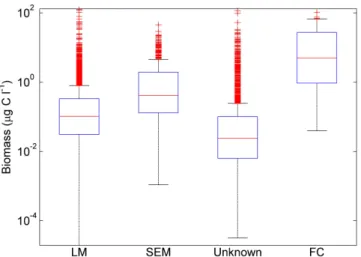
Figure 1.Boxplots depicting distributions of non-zero biomass estimates for different quantification methods: light microscopy (LM), scanning electron microscopy (SEM), unknown method and flow cytometry (FC). Horizontal lines depict the median, boxes depict the interquartile range (25th to 75th percentiles) and points marked beyond the whiskers of the plot are outliers (points falling greater than 1.5 times the interquartile range below the 25th percentile or above the 75th percentile).

18

Figure 1.Boxplots depicting distributions of non-zero biomass

es-timates for different quantification methods: light microscopy (LM), scanning electron microscopy (SEM), unknown method and flow cytometry (FC). Horizontal lines depict the median, boxes depict the interquartile range (25th to 75th percentiles) and points marked beyond the whiskers of the plot are outliers (points falling greater than 1.5 times the interquartile range below the 25th percentile or above the 75th percentile).

et al. (2002) found that species such as syracosphaerids, small reticulofenestrids, small gephyrocapsids and holococ-colithophores are likely to be missed in light microscopy analyses. Cell density has been shown to differ up to 23 % between the two methods when analysing samples with large numbers of small species such as E. huxleyi, Gephyrocapsa ericsonii and G. protohuxleyi.

We have made a statistical comparison of abundance and biomass values to determine whether a systematic bias can be associated with the enumeration method for samples in our database (Table 3, Fig. 1). Our comparison of coccol-ithophore abundance and biomass shows greater differences between methods than would be expected from previous comparisons of enumeration methods, but we suggest that these differences are likely to be at least partially explained by real differences in coccolithophore abundance and com-munity composition. For example, we expect that SEM is more likely to be used for samples with a known portion of small coccolithophores which are difficult to identify or enumerate using light microscopy alone. Although median biomass from SEM studies is higher by a factor of four than the median for light microscopy studies, the highest values reported in the dataset are from light microscopy studies. Since the quantification method is unknown for nearly 50 % of samples, we have chosen to retain SEM data in the gridded dataset and all analyses, though users may access a subset of this data from the raw file. In contrast, we have excluded 199 datapoints collected using flow cytometry from the grid-ded dataset. These values are significantly higher again than those collected using either SEM or light microscopy.

Figure 2.Global distribution of coccolithophore observations included in the dataset. Marker colour denotes the quantification method used: light microscopy (green), SEM (red), flow cytometry (cyan) and unknown (blue)

Figure 3.Distribution of coccolithophore biomass (µgCl−1_{) (a) as a function of latitude and (b) as a function of depth.}

19

Figure 2.Global distribution of coccolithophore observations

in-cluded in the dataset. Marker colour denotes the quantification method used: light microscopy (green), SEM (red), flow cytome-try (cyan) and unknown (blue)

Table 3.Biomass estimates (µgCL−1_{) for four analysis methods:}

light microscopy (LM), scanning electron microscopy (SEM), flow cytometry (FC) and unreported analysis method (unknown). All val-ues are reported for non-zero biomass estimates only.

Method n Median Mean St. Dev. Max LM 4209 0.10 0.72 4.38 126.5

SEM 500 0.41 2.25 4.41 45.2

FC 197 5.04 14.66 18.29 105.5 Unknown 4287 0.024 0.39 2.96 116.0

Based on our full quality control procedure we removed a total of 888 flagged samples for the purposes of our anal-yses, and a further 32 samples were corrected to remove the contribution of T. heimii to total coccolithophore biomass (note: one sample contained data for T. heimii only). All data are included in the published raw dataset in the event that a user has different requirements for the quality control pro-cedure, while the gridded dataset contains the unflagged dat-apoints only.

An additional column in the raw dataset denotes the taxo-nomic level to which coccolithophores are identified, as this has a major influence on the level of uncertainty associated with our biomass calculations. Coccolithophores identified to species level are denoted by the flag value 0, those identi-fied to genus or family level as flag value 1, and unidentiidenti-fied coccolithophores as flag value 3. If coccosphere dimensions are known, cells identified to genus or family level receive flag value 2, and unidentified coccolithophores receive flag value 4. All samples of unidentified or partially identified coccolithophores have been included in our analyses and in the gridded file.

Several datasets report biomass values in addition to abun-dance data. While we have chosen to use our own conver-sion methods for consistency, it is likely that the original biomass values are based on more accurate estimates of cell size. All original biomass values are included in the sub-mitted database and can be substituted for our estimates if desired.

(8)

Figure 2. Global distribution of coccolithophore observations included in the dataset. Marker colour denotes the quantification method used: light microscopy (green), SEM (red), flow cytometry (cyan) and unknown (blue)

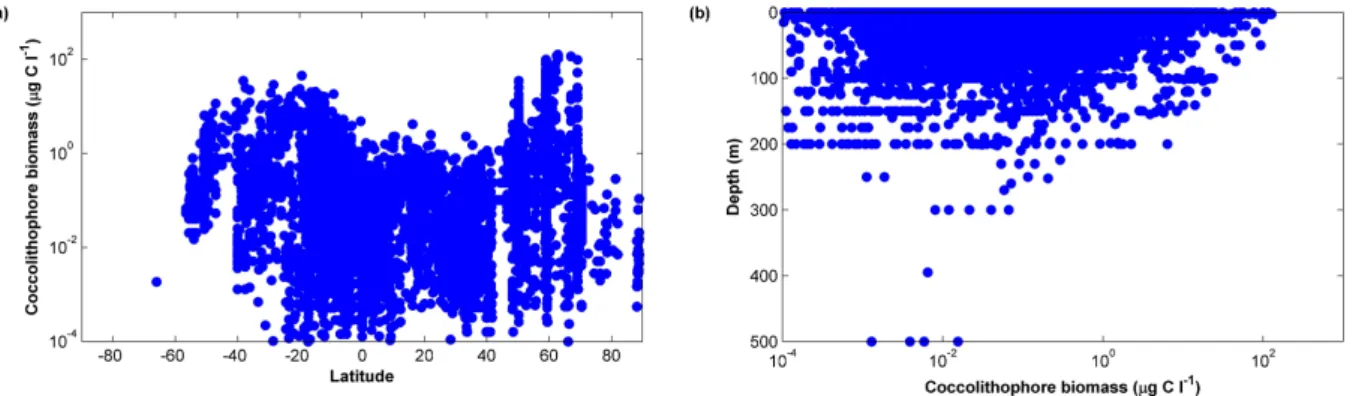
Figure 3.Distribution of coccolithophore biomass (µgCl−1_{) (a) as a function of latitude and (b) as a function of depth.}

19

Figure 3.Distribution of coccolithophore biomass (µgCL−1_{) (a) as a function of latitude and (b) as a function of depth.}

3 Results

Excluding flagged data, the database contains cocithophore biomass observations for 11 503 samples, col-lected from 6741 depth-resolved stations (Fig. 2). Highest coccolithophore abundance is 9.8 × 106cells L−1. 2507, or 21.8 % of samples, were found to be zero values. These data were retained in the dataset, since confirmed zero values hold valuable information for the study of plankton distributions. There is, however, inconsistency in the reporting of zero val-ues in plankton datasets: often abundance data are reported only for a limited range of target groups that are expected to be present. There is also likely to be a bias due to sam-pling focusing on areas where coccolithophores are expected to occur. Values reported in the subsequent sections are there-fore calculated based on non-zero data only. Where zero-datapoints are included, this value follows in parentheses. Arithmetic mean values are reported plus or minus one stan-dard deviation. We also provide median biomass values, as these are less influenced by high values and provide a better representation of the central tendency of the data.

3.1 Spatial and temporal coverage

The database includes non-zero coccolithophore observa-tions from the surface to a depth of 500 m (Fig. 3b, with 83.9 % of observations (84.1 % with zero values included) from the upper 50 m and 61.5 % (63.3 %) from the upper 10 m of the water column. Mean depth is 27.0 (±40.5) m and median depth is 10.0 m. Data are reported from all ocean basins, with 54.4 % of samples (58.9 % with zero values in-cluded) from the Northern Hemisphere and 45.4 % (40.9 %) from the Southern Hemisphere (Table 4). 31.6 % of non-zero data are from the Atlantic Ocean, 40.2 % from the Pa-cific Ocean and 10.4 % from the Indian Ocean. Despite the high number of observations reported from the Pacific com-pared to the Atlantic, the spatial coverage of this ocean basin is relatively poor, with many observations limited to inten-sively studied regions in Peruvian and Japanese coastal wa-ters. 9.9 % of non-zero observations are from the polar

re-Figure 4.Frequency distribution of coccolithophore observations as a function of latitude for the period 1929–2008.

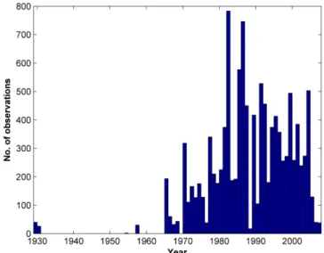
Figure 5.Frequency distribution of coccolithophore observations by year, for the period 1929–2008.

20

Figure 4.Frequency distribution of coccolithophore observations

as a function of latitude for the period 1929–2008.

gions, with 5.1 % from the Southern Ocean and 4.8 % from Arctic waters. Coccolithophores are reported to be present in only one sample below 60◦S (Table 5, Fig. 4). In contrast, the database contains non-zero observations of coccolithophores in Arctic waters up to a maximum of 88.92◦_{N. 46.3 % of} data are from tropical waters between 20◦_{S and 20}◦_N.

Data are reported from the years 1929 to 2008 (Fig. 5). A total of 66 non-zero observations are reported for 1929– 1930, with no further observations until 1954. 78.7 % of observations were collected between 1980 and 2008, and 51.8 % between 1990 and 2008. Data are reported from all months of the year in both hemispheres, although relatively few data were collected during the winter months (13.6 % of all NH data, 15.6 % of SH data, Table 4). Northern Hemi-sphere data are strongly biased towards summer observations (38.4 % of all data).

(9)

Table 4.Seasonal distribution of abundance data for the Northern

and Southern Hemisphere. Number of data points for each month. All: all data, non-zero: data with non-zero carbon biomass.

Month Globe Globe NH NH SH SH all non-zero all non-zero all non-zero Jan 737 367 489 177 247 189 Feb 1271 922 389 260 881 662 Mar 872 729 489 367 383 362 Apr 942 793 433 317 500 467 May 1095 935 634 534 461 401 Jun 944 607 694 394 246 213 Jul 1203 859 1056 734 146 125 Aug 1053 942 697 607 356 335 Sep 1111 1005 810 728 290 266 Oct 1304 975 699 441 605 534 Nov 752 671 245 196 507 475 Dec 219 191 59 50 160 141 Spring – – 1556 1218 1402 1275 Summer – – 2447 1735 1288 992 Autumn – – 1754 1365 1344 1230 Winter – – 937 487 748 673 Total 11 503 8996 6694 4805 4782 4170 3.2 Biomass distribution 3.2.1 Geographical distribution

Coccolithophore biomass values range from 2.0 × 10−5 to 127.2µgCL−1_{. The global mean is 0.88}_µgCL−1 _± 4.8µgCL−1_{and median biomass is 0.072}_µgCL−1_{. Highest} median biomass values were recorded in the Southern Hemi-sphere between 40 and 50◦_{S (0.77, Figs. 3, 6, Table 5), and in} the Northern Hemisphere between 50 and 60◦_{N. Maximum} biomass values show peaks around 60◦_{N and between 40 and} 20◦_{S, with declines towards both the equator and the poles.} Biomass estimates between the equator and 40◦_{N are below} 5µgCL−1_{. The highest biomass estimate of 127.2}_µgCL−1_is for a sample off the Icelandic coast (62.8◦N, 20.0◦W).

Strong differences can be observed between the Atlantic and Pacific Ocean, with Atlantic biomass values reaching 127.2µgCL−1(mean 1.7 ± 7.5, median 0.12µgCL−1) com-pared to just 20.0µgCL−1 in the Pacific (mean 0.3 ± 0.9, median 0.04µgCL−1). The relatively poor spatio-temporal coverage of Pacific Ocean observations, however, may con-tribute to this discrepancy. Indian Ocean biomass values reach a maximum of 45.2µgCL−1_{, with a mean of 1.1 ± 3.4} and median of 0.03µgCL−1_.

In the Southern Ocean, the maximum biomass value re-ported is 6.5µgCL−1_{, mean biomass is 0.19 ± 0.58}_µgCL−1 and median biomass is 0.04µgCL−1_{. Higher values are} recorded in the Arctic Ocean, with a maximum of 98.9µgCL−1_{, mean of 0.78 ± 5.7}_µgCL−1 _{and median of} 0.05µgCL−1.

Figure 4.Frequency distribution of coccolithophore observations as a function of latitude for the period 1929–2008.

Figure 5.Frequency distribution of coccolithophore observations by year, for the period 1929–2008.

20

Figure 5.Frequency distribution of coccolithophore observations

by year, for the period 1929–2008.

3.2.2 Depth distribution

Highest biomass values are reported in surface waters and decline with depth (Figs. 3b, 6), although biomass values of up to 23µgCL−1are still reported at 100 m depth. Mean biomass for the surface layer (0–10 m) is 0.9 ± 5.2µgCL−1 and median biomass is 0.09µgCL−1. Biomass values be-low 200 m reach a maximum of 0.01µgCL−1. The deepest observations of coccolithophores are at 500 m depth, with biomasses reaching a maximum of just 0.004µgCL−1_.

3.2.3 Seasonal distribution

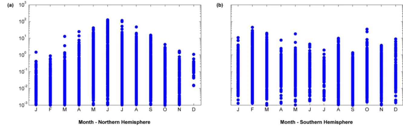
The data show a clear seasonal cycle in the Northern Hemi-sphere, with biomass values reaching just 1.1µgCL−1in De-cember and over 100µgCL−1in the summer months (June– July, Fig. 7). In the Southern Hemisphere the seasonal cycle is less evident, possibly due to the greater contribution of data from low latitudes where seasonal changes are less pro-nounced.

3.2.4 Uncertainty

The expected uncertainty associated with our conversions of cell abundance to carbon biomass due to varying cell size is depicted in Fig. 8. Biomass estimates are best constrained where detailed taxonomic information is available, and for samples containing species for which a limited size range has been reported. Very high uncertainty (range of biomass values greater than 5000 % of the mean biomass) is associ-ated with counts of unidentified coccolithophores. This is to be expected given the large range of sizes reported for the approximately 200 known coccolithophore species (see Ap-pendix Table A3).

(10)

Figure 6.Mean coccolithophore carbon biomass (µgCL−1_{) for six depth bands (a) 0–5 m (b) 5–25 m (c) 25–50 m (d) 50–75 m (e) 75–100 m}

and (f) > 100 m depth.

Figure 7.Seasonal distribution of coccolithophore biomass data for (a) Northern Hemisphere and (b) Southern Hemisphere.

22

Figure 7.Seasonal distribution of coccolithophore biomass data for (a) Northern Hemisphere and (b) Southern Hemisphere.

(11)

Table 5.Latitudinal distribution of quality-controlled data in ten degree latitudinal bands (−90 to 90◦

). All data: total number of data points; non-zero data: number of non-zero biomass values; mean, standard deviation, median and maximum biomass values calculated from non-zero data only.

Latitudinal band All data Non-zero data Mean S.D. Median Max

−90– −80◦ ₀ ₀ _– _– _– _– −80– −70◦ 60 0 – – – – −70– −60◦ 66 1 0.002 – 0.002 0.002 −60– −50◦ 480 456 0.2 0.5 0.04 6.5 −50– −40◦ 116 77 1.8 2.4 0.77 12.3 −40– −30◦ 231 207 1.1 3.7 0.19 35.1 −30– −20◦ 256 247 2.0 4.0 0.16 29.1 −20– −10◦ 1754 1467 0.7 2.2 0.09 45.2 −10– 0◦ 1819 1715 0.2 0.7 0.05 18.4 0–10◦ ₁₀₅₅ ₈₆₀ _0.1 _0.2 _0.03 _2.3 10–20◦ 502 315 0.2 0.4 0.09 4.2 20–30◦ 759 420 0.1 0.2 0.02 2.5 30–40◦ 1340 773 0.1 0.1 0.01 2.3 40–50◦ 804 505 0.3 0.7 0.10 11.5 50–60◦ 1564 1319 2.7 7.8 0.32 99.3 60–70◦ 451 451 3.7 14.7 0.10 127.2 70–80◦ ₂₀₉ ₁₄₆ _0.1 _0.1 _0.05 _0.8 80–90◦ 37 37 0.02 0.05 0.007 0.3

An additional source of uncertainty, however, is the esti-mation of cell biovolumes from coccosphere dimensions, and is more difficult to quantify. A comparison of our biomass estimates based on coccosphere dimensions with estimates from available cytoplasm dimensions suggests that we may be underestimating coccolithophore biomass values by a factor of up to 5 for some species (Table 2). It is worth noting, however, that the cytoplasm dimensions considered here are based on either culture specimens (Stoll et al., 2002) or a small number of field samples from the Icelandic Basin (Poulton et al., 2010) and the Mauritanian Upwelling (Franklin et al., 2009). For one of the best-studied species, E. huxleyi, our mean biomass estimate of 13 pg C cell−1falls within the range of published carbon measurements of 7.8 to 27.9 pg C cell−1(Fernandez et al., 1993; van Bleijswijk et al., 1994; Verity et al., 1992), while our estimates from the cyto-plasm measurements in Table 2 show much lower values of 3.5–3.7 pg C cell−1_.

4 Discussion

There are many sources of uncertainty associated with our calculations. We have attempted to quantify the uncertainty associated with variable cell dimensions by providing mini-mum and maximini-mum biomass values for each datapoint, but this does not represent the full range of uncertainty associ-ated with our biomass values.

The estimation of cell biovolumes from coccosphere di-mensions is likely to result in additional errors which are at present difficult to quantify. A more accurate

estima-tion of coccolithophore biomass will only be possible with improved understanding of coccolithophore cytoplasm di-mensions (e.g. Stoll et al., 2002), and we highlight this as a key data requirement for improved estimates of coccol-ithophore biomass from abundance data. While the routine measurement of coccolithophore cell dimensions is a time-consuming process, there also appears to be potential to esti-mate cell size from coccolith length (Henderiks and Pagani, 2007; Henderiks, 2008).

Few observations of coccosphere dimensions are reported in the literature for most species, and the number of cells that have been studied to derive the given ranges is rarely reported. Measurements are often from a single geographi-cal location, meaning that size variation between strains is not accounted for. There is additionally inconsistency as to whether the range of coccosphere sizes reported is the full range of sizes that occurs or only those most commonly ob-served. A further source of uncertainty is the generalisation of at times complex geometry to fit a particular geometric form.

The uncertainty ranges provided around our biomass esti-mates are intended to reflect the influence of cell size on coc-colithophore biomass. Since these are based on cytoplasm dimensions estimated from total coccosphere size, it is un-clear whether biomass values towards the high end of our uncertainty range are biologically realistic. We may expect larger coccospheres to be characterised by a greater propor-tion of inorganic carbon rather than reflecting a constant ratio of cytoplasm : coccosphere dimensions.

(12)

Figure 8.(a) Surface (0–5 m) mean coccolithophore biomass (µgCl−1

) and (b) range of uncertainty in cell biomass estimates (% of the mean) due to uncertainty in cell size.

23

Figure 8. (a) Surface (0–5 m) mean coccolithophore biomass

(µgCL−1_{) and (b) range of uncertainty in cell biomass estimates}

(% of the mean) due to uncertainty in cell size.

While our uncertainty ranges are very high, a compari-son of our mean biomass estimates to previously published coccolithophore biomass values shows strong consistency: our highest mean biomass estimates (i.e., those associated with large E. huxleyi blooms: maximum of 127µgCL−1) are similar to past estimates from light microscopy-based cell counts (e.g. Holligan et al., 1993: 130µgCL−1), but slightly lower than coccolithophore biomass estimates from fatty acid biomarkers in mesocosm experiments (de Kluijver et al., 2010: 190µgCL−1).

In addition to the errors introduced by the biomass conver-sion process, a considerable degree of uncertainty is already associated with the cell abundance data. Coccolithophores can be quantified using several techniques, including vi-sual or automated identification from scanning electron mi-croscopy, regular light microscopy and light microscopy us-ing cross-polarised light. Additionally, samples can be pre-pared for light microscopy either by filtration or by us-ing the Uterm¨ohl sedimentation method (Uterm¨ohl, 1958). Reid (1980) and Bollmann et al. (2002) both concluded that

inverted light microscopy is unreliable for determining cell densities of small coccolithophores.

Despite these limitations, the Uterm¨ohl method of sed-imentation and inverted light microscopy remains widely used in studies investigating phytoplankton assemblages, and any compilation of global coccolithophore distributions would be incomplete without these data. Cell counts from SEM can additionally be unreliable at high cell densities, where shedded coccoliths can lead to difficulties in distin-guishing individual coccospheres (A. Poulton, personal ob-servation). The synthesis of datasets obtained from these dif-ferent methods would be greatly improved by further com-parative studies similar to those carried out by Bollmann et al. (2002), as it is currently unclear to what extent small and rare species are being overlooked in different ocean re-gions as a result of these methodological differences.

Users of the gridded data file should also take into consid-eration the sparse nature of the original data. Often monthly mean gridded values have been derived from relatively few individual datapoints that do not represent the full range of values that occur in a given location. We expect to see a bias toward higher biomass values, given that studies are often conducted in locations and times of year when blooms are expected to occur.

We have not included estimates of inorganic carbon con-tent in the database, as we do not feel that useful estimates of coccolithophore calcite can currently be provided from the abundance data. The ratio of inorganic : organic carbon has been shown to vary considerably with environmental and growth conditions (Zondervan, 2007), with ratios for the species E. huxleyi alone ranging from 0.26 to 2.3 (van Blei-jswijk et al., 1994; Paasche, 2002). While some estimates have been made of the relationship between inorganic and organic carbon for E. huxleyi-dominated communities (e.g. Fern´andez et al., 1993; Poulton et al., 2010), the relationship of calcite content to biomass for other coccolithophore com-munities remains less well understood.

The biomass estimates presented here represent a first attempt to assess global coccolithophore biomass distribu-tions. While we recognise that the uncertainties associated with these biomass estimates are significant, we neverthe-less feel that they provide a more informative dataset than would a compilation of abundance data alone given the large size variation among coccolithophore species. The coccol-ithophores present particular challenges for the compilation and synthesis of diverse datasets due to the wide range of methods used for their quantification as well as the limited understanding of cell dimensions. The strong biases associ-ated with the different methods highlight the need for coc-colithophore abundance data to be published alongside ap-propriate metadata to allow users to assess data quality.

(13)

5 Conclusions

This database represents the largest effort to date to compile coccolithophore abundance observations and provide stan-dardised biomass estimates to the scientific community. We report our biovolume and biomass conversion procedures in detail and discuss the associated uncertainties. We anticipate that this dataset, together with others from the MAREDAT special issue, will be a valuable resource for studies of plank-ton distributions and ecology and in particular for the evalu-ation and development of marine ecosystem models. While data are clearly lacking for certain regions, the dataset never-theless represents the largest available compilation of global coccolithophore abundance and biomass. We hope to im-prove the spatial and temporal coverage of the dataset as well as the accuracy of biomass conversions as additional data be-come available in the future.

Appendix A

A1 Data table

A full data table containing all biomass data points can be downloaded from the data archive PANGAEA (doi:10.1594/PANGAEA.785092). The data file contains longitude, latitude, depth, sampling time, abundance counts and biomass concentrations, as well as the full data refer-ences.

A2 Gridded netcdf biomass product

Monthly mean biomass data have been gridded onto a 360 × 180◦_{grid, with a vertical resolution of 33 depth levels} (equiv-alent to World Ocean Atlas depths) and a temporal resolution of 12 months (climatological monthly means). This dataset is provided in netcdf format for easy use in model evalua-tion exercises. The netcdf file can be downloaded from PAN-GAEA (doi:10.1594/PANGAEA.785092). This file contains total and non-zero abundance and biomass values. For all fields, the means, medians and standard deviations result-ing from multiple observations in each of the 1◦ pixels are given. The ranges in biomass values due to uncertainties in cell size are not included as variables in the netcdf product, but are given as ranges (minimum cell biomass, maximum cell biomass) in the data table.

(14)

A3 Biomass conversion details

Table A3. Biomass conversion details for coccolithophore taxa reported in the database: biovolume category (best available taxonomic

description, species names corrected where possible); number of datapoints (n, flagged and unflagged data); coccosphere shape (S= sphere,

PS= prolate spheroid, C = cone, CY = cylinder, DC = double cone, V = various shapes, L = species dimensions unknown, cell biovolume

estimate from literature); minimum, maximum and mean coccosphere dimensions (µm), cell biovolume (µm3_{) and cell biomass (pg C L}−1_).

Biovolume Category n Shape Diameter (µm) Length (µm) Width (µm) Biovolume (µm3₎ _{Biomass (pg C cell}−1₎ _References

Min Max Mean Min Max Mean Min Max Mean Min Max Mean Min Max Mean

Acanthoica sp. 199 PS 61 126 85 9 18 12 Acanthoica acanthifera 130 PS 6.0 7.0 6.5 5.0 5.0 5.0 17 20 18 3 3 3 4, 16 Acanthoica janchenii 5 PS 7.0 6.5 17 70 33 3 10 5 16 Acanthoica ornata 4 PS 14.0 16.0 15.0 11.0 12.0 11.5 192 261 224 26 34 30 26 Acanthoica quattrospina 1446 PS 7.0 15.0 11.0 5.0 9.5 7.3 20 153 65 3 21 10 4, 9, 10, 11, 12, 16 Algirosphaera cucullata 25 S 8.0 11.0 9.5 58 151 97 9 21 14 4, 16 Algirosphaera robusta 448 S 6.5 16.0 11.3 31 463 161 5 57 22 4, 9, 10, 11, 12, 16, 25 Alisphaera sp. 60 S 75 211 125 11 28 18 Alisphaera extenta 45 S 6.5 10.0 8.3 31 113 64 5 16 10 17 Alisphaera gaudii 45 S 11.0 12.0 11.5 151 195 172 21 26 23 17 Alisphaera ordinata 67 S 10.0 12.0 11.0 113 195 151 16 26 21 17 Alisphaera pinnigera 70 S 7.0 13.0 10.0 39 248 113 6 32 16 4, 17 Alisphaera spatula 25 S 11.0 75 316 151 11 40 21 5 Alisphaera unicornis 165 S 7.3 12.0 9.7 44 195 102 7 26 15 4, 9, 10, 22 Alveosphaera bimurata 67 DC 18.0 8.0 33 137 65 5 19 10 22 Anacanthoica acanthos 50 PS 8.0 12.5 10.3 7.0 7.0 7.0 44 69 57 7 10 9 4, 11, 16, 26 Anacanthoica cidaris 25 S 13.0 124 522 248 17 63 32 16 Anthosphaera sp. 305 S 4.5 16.0 10.3 10 463 122 2 57 17 4, 10, 18 Anthosphaera fragaria 141 S 4.5 7.0 5.8 10 39 22 2 6 4 4, 10, 18 Braarudosphaera sp. 6 S 5.0 16.0 10.5 14 463 131 2 57 18 Braarudosphaera bigelowii 1034 S 5.0 16.0 10.5 14 463 131 2 57 18 8, 10 Calcidiscus sp. 83 S 5.0 28.0 16.5 64 1432 364 10 157 46 Calcidiscus leptoporus 967 S 5.0 28.0 16.5 14 2483 508 2 257 62 4, 9, 10, 11, 15 Calcidiscus quadriperforatus 67 S 10.0 15.0 12.5 113 382 221 16 48 29 4, 10, 11 Calcioconus sp. 7 C 15.0 18.0 16.5 10.0 12.0 11.0 85 147 113 12 20 16 Calcioconus vitreus 17 C 15.0 18.0 16.5 10.0 12.0 11.0 85 147 113 12 20 16 26 Calciopappus sp. 122 C 18 44 29 3 7 5 Calciopappus caudatus 49 C 26.0 36.0 31.0 3.5 4.0 3.8 18 33 25 3 5 4 10 Calciopappus rigidus 181 C 9.0 12.0 10.5 6.0 9.0 7.5 18 55 33 3 8 5 4, 10, 12 Calciosolenia sp. 61 V 31 817 240 5 95 31 Calciosolenia brasiliensis 1394 DC 33.0 100.0 66.5 4.0 8.0 6.0 30 362 135 5 46 19 1, 4, 9, 10, 12, 19 Calciosolenia murrayi 1311 CY 3.0 10.0 6.5 21.0 75.0 48.0 32 1272 344 5 141 43 1, 4, 9, 10, 11, 12 Calicasphaera blokii 45 S 6.5 7.7 7.1 31 52 40 5 8 6 15 Calicasphaera concava 45 S 7.0 11.0 9.0 39 151 82 6 21 12 15 Calicasphaera diconstricta 25 S 6.2 8.5 7.4 27 69 45 4 10 7 15 Calyptrolithina divergens 67 PS 5.5 8.0 6.8 5.5 6.0 5.8 19 33 25 3 5 4 10 Calyptrolithina multipora 92 S 13.9 22.5 18.2 304 1288 682 39 143 80 10, 15 Calyptrolithina wettsteinii 45 PS 12.5 15.8 14.2 10.7 13.0 11.9 162 302 225 22 39 30 11, 15 Calyptrolithophora gracillima 1 PS 9.5 18.0 13.8 9.0 16.0 12.5 87 521 243 13 63 32 4, 10 Calyptrolithophora papillifera 141 S 9.0 20.0 14.5 82 905 345 12 104 44 4, 10, 11 Calyptrosphaera sp. 820 S 5.0 22.0 13.5 254 484 350 33 59 44 Calyptrosphaera globosa 4 S 17.0 20.0 18.5 556 905 716 67 104 84 26 Calyptrosphaera incisa 1 S 10.0 57 238 113 9 31 16 26 Calyptrosphaera insignis 8 S 11.0 14.0 12.5 151 310 221 21 40 29 26 Caneosphaera sp. 15 S 4.5 18.0 11.3 10 660 161 2 78 22 4, 9, 10, 11, 22 Canistrolithus sp. 74 S 14.3 23.8 19.0 327 1515 776 42 165 90 4 Ceratolithus sp. 6 S 7.0 18.9 13.0 39 764 246 6 89 32 Ceratolithus cristatus 107 S 7.0 18.9 13.0 39 764 246 6 89 32 4, 10, 22 Coccolithus sp. 1191 S 8.0 22.0 15.0 58 1204 382 9 134 48 Coccolithus pelagicus 1108 S 8.0 22.0 15.0 58 1204 382 9 134 48 9, 10, 11

Coccolithus pelagicus holo 625 S 8.0 18.0 13.0 58 660 248 9 78 32 10

Corisphaera sp. 40 S 4.5 9.2 6.9 15 52 28 3 8 5 Corisphaera gracilis 93 S 6.5 16 65 31 3 10 5 10 Corisphaera strigilis 49 S 5.0 7.0 6.0 14 39 24 2 6 4 4 Coronosphaera sp. 626 S 12.0 53.0 32.5 222 509 345 29 62 44 Coronosphaera binodata 4 S 13.0 16.0 14.5 248 463 345 32 57 44 4, 26 Coronosphaera mediterranea 544 S 12.0 17.0 14.5 195 556 345 26 67 44 4, 9, 10 Cribrosphaera sp. 15 S 8.3 32 136 65 5 19 10 23 Cribrosphaera ehrenbergii 5 S 8.3 32 136 65 5 19 10 23 Crystallolithus sp. 11 S 8.0 20.0 14.0 58 905 310 9 104 40 10 Cyrtosphaera aculeata 93 S 7.0 19 81 39 3 12 6 4, 10, 16 Cyrtosphaera lecaliae 45 S 9.0 41 173 82 6 23 12 16 Discosphaera sp. 152 S 4.5 14.0 10.0 10 310 113 2 40 16 Discosphaera tubifera 1312 S 4.5 14.0 10.0 10 310 113 2 40 16 1, 4, 9, 10, 11, 12, 16 Emiliania huxleyi 5651 S 3.5 15.0 9.3 5 382 90 1 48 13 1, 4, 9, 10, 11, 12, 14, 22

Florisphaera profunda var. elongata 49 S 12.0 98 410 195 14 51 26 4, 10, 12, 24, 25

Florisphaera profunda var. profunda 536 S 4.0 12.0 8.0 7 195 58 1 26 9 25

Gephyrocapsa sp. 909 S 2.6 15.0 8.8 22 121 50 4 17 8 Gephyrocapsa ericsonii 254 S 3.0 5.0 4.0 3 14 7 1 2 1 4, 9, 10, 25 Gephyrocapsa muellerae 49 S 7.0 8.0 7.5 39 58 48 6 9 7 4 Gephyrocapsa oceanica 933 S 5.0 15.0 10.0 14 382 113 2 48 16 4, 6, 9, 10, 11, 12 Gephyrocapsa ornata 422 S 3.3 4.5 3.9 31 31 31 5 5 5 4, 10 Gephyrocapsids 9 S 2.6 15.0 8.8 19 165 56 3 22 9 Gladiolithus flabellatus 245 S 8.0 12.0 10.0 58 195 113 9 26 16 4

(15)

Table A3. Continued.

Halopappus sp. 582 V 65 273 132 10 35 18 Halopappus quadribrachiatus 6 S 5.0 8.0 6.5 14 58 31 2 9 5 26 Halopappus vahseli 8 C 21.0 14.0 116 489 233 16 60 31 26 Heimiella excentrica 18 S 18.0 24.0 21.0 660 1563 1047 78 170 118 26 Helicosphaera sp. 398 V 150 672 340 21 79 43 Helicosphaera carteri 553 PS 10.0 28.0 19.0 13.0 20.0 16.5 191 1267 585 26 140 70 1, 4, 9, 10, 11, 12

Helicosphaera carteri (holo) 67 S 10.0 15.5 12.8 113 421 234 16 52 31 4, 11

Helicosphaera hyalina 109 PS 12.0 22.0 17.0 11.0 18.0 14.5 164 806 404 22 94 50 4, 10, 12 Helicosphaera pavimentum 131 PS 10.5 13.5 12.0 10.5 12.5 11.5 131 239 179 18 31 24 4, 22 Helicosphaera wallichii 49 S 14.7 13.4 149 627 299 21 75 38 4, 22 Helladosphaera sp. 60 PS 4.9 9.0 7.0 4.0 6.4 5.2 9 42 21 2 7 4 Helladosphaera cornifera 158 PS 4.9 9.0 7.0 4.0 6.4 5.2 9 42 21 2 7 4 4, 10, 11 Holococcolithophora sphaeroidea 100 S 6.0 12.0 9.0 24 195 82 4 26 12 4, 10 Homozygosphaera sp. 45 S 6.0 15.0 10.5 41 315 131 6 40 18 Homozygosphaera arethusae 45 S 6.0 15.0 10.5 24 382 131 4 48 18 4 Homozygosphaera triarcha 92 S 8.0 13.0 10.5 58 248 131 9 32 18 4, 10 Lohmannosphaera sp. 4 S 6.0 12.0 9.0 24 195 82 4 26 12 1, 9, 10, 11, 12, 25, 26 Lohmannosphaera adriatica 32 S 10.0 12.0 11.0 113 195 151 16 26 21 1, 9, 10, 11, 12, 25, 26 Lohmannosphaera paucoscyphos 18 S 8.0 29 122 58 5 17 9 26 Michaelsarsia sp. 18 V 77 573 247 11 69 32 Michaelsarsia adriaticus 270 PS 10.0 30.0 20.0 8.0 15.0 11.5 72 763 299 11 89 38 1, 9, 10, 11, 12, 25, 26 Michaelsarsia elegans 200 S 9.0 15.0 12.0 82 382 195 12 48 26 4, 9, 10 Michaelsarsia splendens 32 S 12.0 98 410 195 14 51 26 25, 26 Navilithus altivelum 45 S 5.0 8.0 6.5 14 58 31 2 9 5 28 Oolithotus sp. 39 S 60 1651 364 9 178 46 Oolithotus antillarum 301 S 10.0 13.0 11.5 113 248 172 16 32 23 4 Oolithotus fragilis 579 S 4.0 30.0 17.0 7 3054 556 1 310 67 4, 9, 10, 22 Ophiaster sp. 101 S 3.5 10.5 7.0 5 131 39 1 18 6 1, 4, 10, 11, 12 Ophiaster hydroideus 1748 S 3.5 8.0 5.8 5 58 22 1 9 4 1, 4, 10, 11, 12 Palusphaera vandelii 145 S 4.0 8.7 6.4 7 74 29 1 11 5 4, 10, 22 Pappomonas sp. 294 V 21 894 1331 4 103 147 Pappomonas flabellifera 25 PS 4.5 7.5 6.0 3.0 5.0 4.0 5 21 11 1 4 2 20, 29 Papposphaera sp. 192 S 4.0 16.0 10.0 9 48 23 2 7 4 Papposphaera borealis 67 S 7.0 7 58 24 1 9 4 21 Papposphaera lepida 165 S 4.5 16.0 10.3 10 39 22 2 6 4 4, 10, 29 Picarola margalefii 94 S 6.0 12.0 9.0 24 195 82 4 26 12 4 Pleurochrysis carterae 32 S 12.0 17.0 14.5 195 556 345 26 67 44 3, 10

Pleurochrysis roscoffensis 8 S 12.0 20.0 16.0 195 905 463 26 104 57 7

Polycrater galapagensis 141 S 9.8 15.8 12.8 106 446 237 15 55 31 4 Pontosphaera sp. 114 V 261 1056 551 34 119 66 Pontosphaera discopora 2 S 17.0 28.0 22.5 556 2483 1288 67 257 143 9, 10 Pontosphaera echinofera 5 PS 16.0 12.0 195 821 391 26 95 49 26 Pontosphaera haeckelli 2 S 11.0 15.0 13.0 151 382 248 21 48 32 26 Pontosphaera inermis 1 S 7.0 9.0 8.0 39 82 58 6 12 9 26 Pontosphaera nigra 42 PS 20.0 24.0 22.0 14.0 16.0 15.0 443 695 560 55 82 67 26 Pontosphaera ovalis 1 S 5.0 6.0 5.5 14 24 19 2 4 3 26 Pontosphaera stagnicola 1 S 14.0 20.0 17.0 310 905 556 40 104 67 26 Pontosphaera syracusana 555 S 15.0 30.0 22.5 382 3054 1288 48 310 143 1, 10 Poricalyptra sp. 45 V 43 200 103 7 27 15 Poricalyptra aurisinae 67 S 7.0 12.0 9.5 39 195 97 6 26 14 4 Poricalyptra magnaghii 92 PS 10.0 13.5 11.8 6.5 11.6 9.1 48 205 109 7 27 15 22 Poritectolithus sp. 70 S 6.8 14.0 10.4 35 310 126 6 40 18 4, 5 Poritectolithus poritectus 70 S 9.0 41 173 82 6 23 12 4 Reticulofenestra parvula 159 S 3.0 3.8 3.4 3 6 4 1 1 1 4, 10 Reticulofenestra sessilis 284 S 6.0 10.5 8.3 24 131 64 4 18 10 9, 22, 25 Rhabdosphaera sp. 295 S 4.0 12.0 8.0 202 252 223 27 33 29 Rhabdosphaera ampullacea 1 S 6.8 7.3 7.1 36 44 40 6 7 6 25 Rhabdosphaera clavigera 1641 S 7.9 12.0 10.0 56 195 111 8 26 16 1, 4, 9, 10, 11, 12, 16 Rhabdosphaera hispida 46 S 10.0 12.0 11.0 113 195 151 16 26 21 26 Rhabdosphaera tignifer 2 L 800 800 800 93 93 93 27 Rhabdosphaera xiphos 212 S 4.0 6.0 5.0 7 24 14 1 4 2 4 Scyphosphaera apsteinii 414 S 18.0 25.0 21.5 660 1767 1124 78 189 126 1, 4, 9, 10, 11, 25 Solisphaera sp. 45 S 5.0 9.4 7.2 17 76 39 3 11 6 Solisphaera blagnacensis 45 S 5.6 9.4 7.5 20 93 48 3 13 7 2 Solisphaera emidasius 45 S 5.0 8.0 6.5 14 58 31 2 9 5 2 Sphaerocalyptra sp. 45 S 5.0 22.0 13.5 14 1204 278 2 134 36 4, 10, 11 Sphaerocalyptra adenensis 71 S 5.5 8.5 7.0 19 69 39 3 10 6 4 Sphaerocalyptra quadridentata 68 S 5.0 9.0 7.0 14 82 39 2 12 6 4, 10, 11 Syracolithus sp. 47 S 10.0 19.0 14.5 113 776 345 16 90 44 Syracolithus dalmaticus 29 S 10.0 19.0 14.5 113 776 345 16 90 44 4, 10 Syracosphaera sp. 1249 S 92 598 246 13 72 32 Syracosphaera ampliora 25 S 5.6 10.2 7.9 20 120 56 3 17 8 4, 22 Syracosphaera anthos 183 S 7.0 13.0 10.0 39 248 113 6 32 16 4, 9, 10

Syracosphaera anthos holo 2 S 15.0 191 802 382 26 93 48 26

Syracosphaera bannockii 112 S 5.0 7.0 6.0 14 39 24 2 6 4 4 Syracosphaera borealis 49 S 6.5 8.2 7.4 31 62 45 5 9 7 22 Syracosphaera brandtii 43 S 12.0 15.0 13.5 195 382 278 26 48 36 26 Syracosphaera corolla 141 S 9.8 11.6 10.7 641 641 641 76 76 76 22 Syracosphaera cupulifera 3 S 10.0 57 238 113 9 31 16 26 Syracosphaera delicata 45 S 6.5 7.5 7.0 31 48 39 5 7 6 4 Syracosphaera dentata 19 S 5.0 17.0 11.0 14 556 151 2 67 21 26 Syracosphaera dilatata 117 S 9.0 14.0 11.5 82 310 172 12 40 23 5

(16)

Table A3. Continued.

Syracosphaera epigrosa 117 S 8.0 13.0 10.5 58 248 131 9 32 18 22 Syracosphaera exigua 94 S 7.5 11.7 9.6 48 181 100 7 24 14 22 Syracosphaera grundii 38 S 8.0 10.0 9.0 58 113 82 9 16 12 26 Syracosphaera halldalii 116 S 6.0 18.0 12.0 24 660 195 4 78 26 4, 9, 10, 22 Syracosphaera histrica 273 PS 10.8 20.0 15.4 9.0 14.0 11.5 99 443 230 14 55 30 10, 22 Syracosphaera lamina 165 PS 12.0 47.0 29.5 12.5 23.5 18.0 212 2936 1081 28 299 122 9, 11, 22 Syracosphaera marginaporata 165 S 3.0 6.0 4.5 3 24 10 1 4 2 5 Syracosphaera molischii 1083 S 4.5 11.3 7.9 10 163 56 2 22 8 4, 9, 10, 11, 22 Syracosphaera nana 106 S 5.5 8.2 6.9 19 62 36 3 9 6 4, 22 Syracosphaera nodosa 248 S 6.5 20.0 13.3 31 905 263 5 104 34 4, 10, 22 Syracosphaera noroitica 70 S 9.0 11.0 10.0 82 151 113 12 21 16 22 Syracosphaera orbiculus 165 S 6.0 9.3 7.7 24 91 51 4 13 8 22 Syracosphaera ossa 141 S 6.0 8.3 7.2 24 65 41 4 10 6 4, 22 Syracosphaera pirus 240 PS 6.0 18.0 12.0 6.0 10.0 8.0 24 204 87 4 27 13 9, 10, 12, 22 Syracosphaera prolongata 511 C 10.0 70.0 40.0 7.0 8.0 7.5 55 507 254 8 62 33 4, 10, 11, 22 Syracosphaera pulchra 1531 PS 5.0 70.0 37.5 10.0 23.0 16.5 57 4188 1155 9 411 129 1, 4, 9, 10, 11, 12

Syracosphaera pulchra (holo) 257 S 8.0 28.0 18.0 58 2483 660 9 257 78 10, 11

Syracosphaera rotula 116 S 5.0 7.2 6.1 14 42 26 2 7 4 4, 10, 22 Syracosphaera schilleri 1 S 15.0 191 802 382 26 93 48 26 Syracosphaera spinosa 2 S 8.0 9.5 8.8 58 97 76 9 14 11 26 Syracosphaera subsalsa 5 PS 20.0 28.0 24.0 14.0 18.0 16.0 443 1026 695 55 116 82 26 Syracosphaera tumularis 94 S 10.0 20.0 15.0 113 905 382 16 104 48 4 Thoracosphaera heimii 33 S 12.0 12.6 12.3 195 226 210 26 30 28 25 Turrilithus latericioides 206 S 8.0 11.0 9.5 58 151 97 9 21 14 4 Umbellosphaera sp. 690 S 9.2 16.0 12.6 101 422 224 14 52 30 Umbellosphaera irregularis 1079 S 10.0 15.0 12.5 113 382 221 16 48 29 9 Umbellosphaera tenuis 420 S 9.2 16.0 12.6 88 463 226 13 57 30 4, 10, 11 Umbilicosphaera sp. 1968 S 8.5 43.0 25.8 84 3825 929 12 379 106 Umbilicosphaera foliosa 46 S 10.0 18.0 14.0 113 660 310 16 78 40 4, 10, 13, 22, 25 Umbilicosphaera hulburtiana 289 PS 8.5 28.0 18.3 8.5 24.0 16.3 69 1824 545 10 195 66 4, 10 Umbilicosphaera sibogae 1601 S 8.5 43.0 25.8 69 8992 1931 10 818 205 1, 4, 9, 10, 11, 12, 22 Zygosphaera sp. 1 S 6.0 15.0 10.5 32 163 80 5 22 12 Zygosphaera amoena 45 S 5.0 7.0 6.0 14 39 24 2 6 4 4 Zygosphaera hellenica 120 S 8.0 15.0 11.5 58 382 172 9 48 23 4, 10, 11, 12, 15, 25 Zygosphaera marsilii 27 S 6.0 8.5 7.3 24 69 43 4 10 7 4, 10

References: (1) Avancini et al. (2006), (2) Bollmann et al. (2006), (3) Bottino (1978), (4) Cros and Fortu˜no (2002), (5) Cros i Miguel (2002), (6) Doan-Nhu and Larsen (2010), (7) Gayral and Fresnel (1976), (8) Hagino et al. (2000), (9) Hallegrae_{ff (1984), (10) Heimdal (1997), (11) Heimdal and Saugestad (2002), (12) Hernandez-Becerril and Bravo-Sierra} (2001), (13) Inouye and Pienaar (1984), (14) Klaveness (1972), (15) Kleijne (1991), (16) Kleijne (1992), (17) Kleijne et al. (2002), (18) Lecal (1967), (19) Malinverno (2004), (20) Manton and Oates (1975), (21) Manton et al. (1976), (22) Okada and McIntyre (1977), (23) Priewalder (1973), (24) Quinn et al. (2005), (25) Reid (1980), (26) Schiller (1930), (27) Vilicic (1985), (28) Young and Andruleit (2006), (29) Young et al. (2003)

Acknowledgements. We wish to thank Philipp Assmy, Greta

Fryxell, Dimitri Gutiérrez, Patrick Holligan, Catherine Jeandel, Ian Joint, Kalliopi Pagou, Sergey Piontkovski, Tatjana Ratkova, Ralf Schiebel, Mary Silver, Paul Tett, Jahn Throndsen and Paul Wassmann for granting permission to use and redistribute coc-colithophore data, the BODC, JGOFS, OBIS, OCB-DMO, PAN-GAEA, WOD09 and the Observatoire Océanologique de Ville-franche databases for providing and archiving data, Erik Buiten-huis for producing the gridded dataset, Scott Doney for assistance with the quality control procedure and Stéphane Pesant for archiv-ing the data. The research leadarchiv-ing to these results has received funding from the European Community’s Seventh Framework Pro-gramme (FP7 2007–2013) under grant agreement number (238366). M. Vogt, J. A. Peloquin and N. Gruber acknowledge funding from ETH Zurich.

Edited by: D. Carlson

References

Ajani, P., Lee, R., Pritchard, T., and Krogh, M.: Phytoplankton dy-namics at a long-term coastal station off Sydney, Australia, J. Coastal Res., 34, 60–73, 2001.

Aktan, Y., Luglie, A., Aykulu, G., and Sechi, N.: Species compo-sition, density and biomass of coccolithophorids in the Istanbul Strait, Turkey, Pak. J. Bot., 35, 45–52, 2003.

Anderson, T. R.: Plankton functional type modelling: running before we can walk?, J. Plankton Res., 27, 1073–1081, doi:10.1093/plankt/fbi076, 2005.

Andruleit, H.: Living coccolithophores recorded during the onset of upwelling conditions off Oman in the western Arabian Sea, J. Nannoplankton Res., 27, 1–14, 2005.

Andruleit, H.: Status of the Java upwelling area (Indian Ocean) dur-ing the oligotrophic Northern Hemisphere winter monsoon sea-son as revealed by coccolithophores, Mar. Micropaleontol., 64, 36–51, doi:10.1016/j.marmicro.2007.02.001, 2007.

Andruleit, H., St¨ager, S., Rogalla, U., and Cepek, P.: Living coc-colithophores in the northern Arabian Sea: ecological tolerances and environmental control, Mar. Micropaleontol., Supplement, 49, 157–181, doi:10.1016/S0377-8398(03)00049-5, 2003. Assmy, P.: Phytoplankton abundance measured on water

bottle samples at stations PS65/424-3, 514-2, 570-4 & 587-1, Alfred Wegener Institute for Polar and Marine Research, Bremerhaven, doi:10.1594/PANGAEA.603388, doi:10.1594/PANGAEA.603393,

doi:10.1594/PANGAEA.603398 and doi:10.1594/PANGAEA.603400, 2007.