Application of optimization techniques to the design and maintenance of satellite constellations

(1)

Application of Optimization Techniques to the

Design and Maintenance of Satellite Constellations

by

James Earl Smith B.S. Astronautical Engineering United States Air Force Academy, 1997

SUBMITTED TO THE DEPARTMENT OF AERONAUTICS AND ASTRONAUTICS IN PARTIAL FULFILLMENT OF THE REQUIREMENTS FOR THE DEGREE OF

MASTER OF SCIENCE IN AERONAUTICS AND ASTRONAUTICS AT THE

MASSACHUSETTS INSTITUTE OF TECHNOLOGY JUNE 1999

The author hereby grants to MIT permission to reproduce and to distribute publicly paper and electronic copies of this thesis document in whole or in part.

Signature of Author:

7

Department of Aeronautics and Astronautics May 7, 1999 Certified by: Certified by: Accepted by: Dr. Ronald J. Proulx 'hets Supervisor, CSDL _ ' Dr. PaulJ. Cefola Thesis Supervisor, CSDL Lecturr, De art t of Aeronautics and Astronautics :~~~~~~~~~~~~~~~am Peraire1 \ --.J It Jaime Peraire

Associate Professor Chairman, Deprtment Graduate Committee

(2)

[This Page Intentionally Left Blank]

(3)

Application of Optimization Techniques to the

Design and Maintenance of Satellite Constellations

by

James Earl Smith

Submitted to the Department of Aeronautics and Astronautics on May 7, 1999 in Partial Fulfillment of the Requirements for the Degree of

Master of Science in Aeronautics and Astronautics ABSTRACT

Optimization techniques were studied and applied to a variety of applications in both the design and maintenance of satellite constellations. Powell's method and parallel genetic algorithms were used in conjunction with precise orbit propagation schemes to develop robust orbit optimization tools.

Specifically, local and global optimization methods were used to design a 113:14 repeat ground track variant of the EllipsoTM inclined elliptical sub-constellation and a gear array variant of the EllipsoTM _{equatorial sub-constellation. The resulting optimal constellation}

designs were found to maintain stability, even when subjected to full perturbation analysis.

The global optimization technique of parallel genetic algorithms was also used to create an optimization approach capable of maintaining the designed orbits over specified lengths of time. Although the global method proved successful over short time periods, limitations of the approach eliminated longer time span optimizations and led to the creation of a more operational station-keeping optimization scheme. The more operational station-keeping implementation yielded similar station-keeping estimates while allowing for the study of longer time periods.

Thesis Supervisor: Dr. Ronald J. Proulx

Title: Principle Member of the Technical Staff, The Charles Stark Draper Laboratory Thesis Supervisor: Dr. Paul J. Cefola

Title: Lecturer, Department of Aeronautics and Astronautics Program Manager, The Charles Stark Draper Laboratory

(4)

(5)

(6)

(7)

ACKNOWLEDGEMENTS

No major piece of work, such as this, is complete without mention of the many people who made its production possible.

First, I would like to express my appreciation to all those at the Charles Stark Draper Laboratory who provided assistance in so many ways. To my advisors, Dr. Ronald J. Proulx and Dr. Paul J. Cefola-your knowledge, inspiration, guidance, and extra motivational "push" when needed will not be forgotten. Thank you for giving me the chance as well as the tools to make the most of that chance.

To the members of the Education Office, John Sweeney, Loretta Mitrano, Arell Maguire, and George Schmidt, thank you for providing me with the opportunity and for paying the bills along the way.

To my office mates and fellow students, both past and present. To Scott Carter, Naresh Shah, Brian Kantsiper, and Joe Neelon-your association has provided me with valuable examples to emulate and your work paved the way for this work to be accomplished. To Jack Fischer and George Granholm who shared the recycled air of my office, as well as frustration with homework and FORTRAN, I couldn't have done it with out some one to complain to. To Geoff Billingsley and Mike Jamoom, it's been a long two years. Thanks for the shared experiences and insight.

To all others at the Draper Laboratory whose efforts, either directly or indirectly made this thesis possible: Tim Brand, Roger Medeiros, Linda Alger, Lee Norris, Neil Dennehy, Paul Johnson, Joe Sarcia and the reprographics department, and many others. Thank You.

Others, outside of the Draper Laboratory also had a significant impact on this work. To John Draim and the Ellipso Corporation, I express my deepest gratitude for everything from technical support to proofreading of papers. It has been a pleasure to work with you.

To all those at MIT whose association was brief but valuable. To Professor Eric Feron for providing me with academic guidance as well as optimization instruction. To Professors Battin, Van der Velde, Strang, and others who somehow let me pass their classes. To Liz Zotos and others in the graduate office for their behind the scenes efforts in behalf of all graduate students.

To the Air Force and members of AFIT staff, especially Capt. Rick Sutter. Thank you for allowing me this chance at civilian life and giving me the support to succeed.

To my parents for imparting to me the desire to do my best in life and for making many sacrifices to allow me to do so. To my brothers, sisters, nieces, and nephew, and to my recently acquired family-the Cromars, your e-mails and visits helped us remember there was life beyond Boston and your encouragement and prayers made all the difference.

(8)

Finally, I would like to thank the most important people in my life. My wife, Kristy, for providing support, friendship, love, and for catching all my stupid errors (both in this thesis and in life). And to my son James, whose entrance into the world in the middle of this whole project reminded me of what really is important in this life. I look forward to the eternities we can share together.

This thesis was prepared at The Charles Stark Draper Laboratory, Inc., with support from Draper Laboratory's DFY98 and 99 IR&D Programs under Astrodynamics IR&D Task 837.

Publication of this thesis does not constitute approval of Draper or the sponsoring agency of the findings or conclusions contained herein. It is published for the exchange and stimulation of ideas.

Permission is hereby granted by the Author to the Massachusetts Institute of Technology to reproduce any or all of this thesis.

James E. Smith, 2 Lt., USAF

(9)

9

(10)

2-3-3-2 Draper Semi-Analytic Satellite Theory Standalone Orbit Propagator ... 63

2-4 PARALLEL PROCESSING ... 65

2-4-1 Parallel Processing Description ... 66

2-4-2 Message Passing Interface (MPI) ... 66

2-4-2-1 History of MPI ... 67

2-4-2-2 MPI Implementations and MPICH ... 68

CHAPTER 3 OPTIMIZATION THEORIES AND TECHNIQUES ... 71

3-1 OPTIMIZATION TERMS AND FUNDAMENTALS ... ... 71

3-2 ANALYTICAL OPTIMIZATION THEORIES ... ... 72

3-2-1 Calculus Concepts ... 73

3-2-1-1 Functions of More than One Variable ... 74

3-2-1-2 Lagrange Multipliers ... 75

3-2-2 Variational Calculus... 76

3-2-2-1 Functionals of More than One Function ... ... 79

3-2-2-2 Variational Approach to Optimal Control Problems ... 80

3-2-2-2-1 Theory Description ... 80

3-2-2-2-2 Primer Vector Theory: An Application of Optimal Control Techniques ... 84

3-3 NUMERICAL METHODS ... 87

3-3-1 Dynamic Programming and Principle of Optimality ... 87

3-3-1-1 Greedy Algorithms ... 88

3-3-1-2 Principle of Optimality ... 89

3-3-2 Localized Methods ... 93

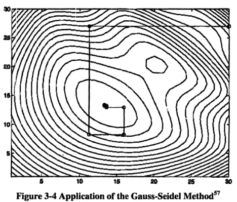
3-3-2-1 Gauss-Seidel Method ... 94

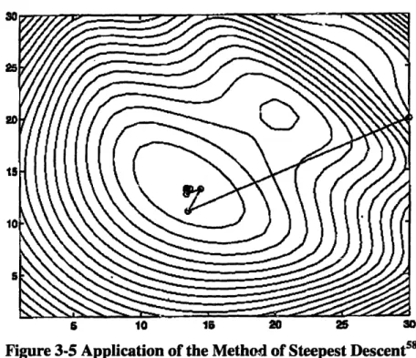
3-3-2-2 Steepest Descent or Gradient Method ... 96

3-3-2-3 Newton's Method ... 97

3-3-2-4 Powell's Method ... 98

3-3-3 Non-localized Approaches ... 99

3-3-3-1 Genetic Algorithms ... 101

(11)

3-3-3-1-2 Cycle of the Genetic Algorithm ... 102

3-3-3-1-3 Mathematical Foundations of the Genetic Algorithm ... 106

3-3-3-1-4 A Computer Implementation of the Genetic Algorithm-PGAPack ... 110

3-3-4 Hybrid Methods ... 112

CHAPTER 4 OPTIMAL CONSTELLATION DESIGN ... 115

4-1 ELLIPSOTM BOREALIS 113:14 REPEAT GROUND TRACK PROBLEM ... 115

4-1-1 113:14 Repeat Ground Track Problem Formulation ... 118

4-1-2 113:14 Repeat Ground Track Localized Solution Process ... 119

4-1-2-1 Powell's Method Program Structure ... ... 120

4-1-2-1-1 113:14 Repeat Ground Track Objective Function Code Structure .. ... 121

4-1-2-1-2 113:14 Repeat Ground Track Propagation Input Parameters .. ... 122

4-1-2-2 Powell's Method Performance on 113:14 Repeat Ground Track Problem ... 123

4-1-2-3 Results of Powell's Method for 113:14 Repeat Ground Track Optimization ... 125

4-1-3 113:14 Repeat Ground Track Genetic Algorithm Solution Process ... 126

4-1-3-1 113:14 Repeat Ground Track Genetic Algorithm Code Structure .. ... 126

4-1-3-1-1 113:14 Repeat Ground Track Variable String Structure ... 129

4-1-3-1-2 113:14 Repeat Ground Track GA Objective Function Structure . ... 130

4-1-3-1-3 113:14 Repeat Ground Track Genetic Algorithm Parameters ... 131

4-1-3-1-4 113:14 Repeat Ground Track Genetic Algorithm Propagation Parameters ... 134

4-1-3-2 Performance of the GA on 113:14 Repeat Ground Track Optimization ... 134

4-1-3-3 Genetic Algorithm Results for 113:14 Repeat Ground Track Optimization ... 136

4-1-4 Performance of Borealis TM With Optimally Designed Elements . ... 136

4-2 ELLIPSOTM GEAR ARRAY DESIGN OPTIMIZATION ... 141

4-2-1 Gear Array Description ... 141

4-2-2 Gear Array Problem Formulation ... ... 143

4-2-2-1 APTS behavior ... 144

4-2-2-2 Commensurability Behavior ... 146

4-2-2-2-1 Geometric or Stroboscopic Constraint ... ... 146

4-2-2-2-2 Period Commensurability or Ratio Constraint ... 149

(12)

4-2-3 Gear Array Solution Process ... ... 151

4-2-3-1 Gear Array Problem Parameterization ... ... 151

4-2-3-2 Gear Array Optimization Code Structure ... ... 155

4-2-3-2-1 Gear Array Genetic Algorithm Variable String Structure ... 155

4-2-3-2-2 Gear Array Objective Function Structure ... 155

4-2-3-2-3 Gear Array Genetic Algorithm Parameters ... ... 157

4-2-3-2-4 Gear Array Propagation Parameters ... ... 158

4-2-4 Genetic Algorithm Performance on Gear Array Design Optimization . ... 159

4-2-5 Results of Gear Array Optimization ... 160

4-2-6 Gear Array Performance ... 161

4-2-6-1 Gear Array Performance Objective Function Analysis ... 161

4-2-6-1-1 Gear Array Design Accuracy ... 162

4-2-6-1-2 Gear Array Orbit Decay Under Full Perturbtions ... 163

4-2-6-2 Gear Array Coverage Analysis ... 166

CHAPTER 5 OPTIMAL CONSTELLATION MAINTENANCE ... 169

5-1 STATION KEEPING PROBLEM FORMULATION ... 169

5-2 PREVIOUS STATION-KEEPING ATTEMPT LIMITATIONS ... ... 171

5-2-1 Simplified Orbit Propagation ... 171

5-2-2 Localized/Greedy Strategy ... 172

5-2-3 Requirement of Pre-defined Targeting Scheme ... 172

5-3 GLOBAL STATION KEEPING APPROACH ... ... 173

5-3-1 Global Station Keeping Implementation ... 174

5-3-1-1 Global Station Keeping Variable Description ... 175

5-3-1-2 Global Station Keeping Objective Function ... 176

5-3-1-3 Global Station Keeping Genetic Algorithm Parameters ... 177

5-3-1-4 Useful Modifications to the Global Station Keeping Implementation ... 179

5-3-1-4-1 Modifications to the Global Station Keeping Objective Function ... 180

5-3-1-4-2 Modifications to the Global Station Keeping Variable Structure ... 182

5-3-1-4-3 Effectiveness of the Global Station Keeping Modifications ... 183

(13)

5-3-1-5 Computer Implementation of the Global Station Keeping Approach ... 183

5-3-1-5-1 Code for Reference Orbit Definition ... ... ... 184

5-3-1-5-2 Code for Time of First Deviation Calculation ... 185

5-3-1-5-3 Objective Function Code Structure (FUNC) ... 185

5-3-2 Global Station Keeping Approach Test Cases ... 187

5-3-2-1 Global Station Keeping Case Descriptions ... 188

5-3-2-1-1 Global Station Keeping Reference Orbit Definition ... 188

5-3-2-1-2 Global Station Keeping Case 1- Epoch Aligned with Reference Elements ... 189

5-3-2-1-3 Global Station Keeping Case 2-Epoch Elements at Extreme Limits ... 191

5-3-2-2 Global Station Keeping Results ... 193

5-3-2-2-1 Case 1 Results-Epoch Elements Aligned with Reference Elements ... 193

5-3-2-2-2 Case 2 Results-Epoch Elements at Extreme Limits ... 196

5-3-3 Global Station Keeping Comparison to ASKS Resuls ... 202

5-3-4 Limitations of the Global Station Keeping Approach ... 204

5-3-4-1 Computational Limitations ... 204

5-3-4-2 Limitation of Ending at Near-Violations ... 205

5-3-4-3 Non-repeatable Limitation ... ... 206

5-3-4-4 Dependence on Propagation Techniques ... 206

5-4 OPERATIONAL STATION KEEPING APPROACH ... ... 207

5-4-1 Definition of Operational Features ... ... 208

5-4-2 Operational Approach Overview ... 209

5-4-3 Implementation of Operational Approach ... 212

5-4-3-1 Operational Approach Variable Description ... 212

5-4-3-2 Operational Approach Objective Function ... 213

5-4-3-3 Operational Approach Genetic Algorithm Parameters ... 216

5-4-3-4 Operational Approach Computer Implementation ... 218

5-4-4 Operational Approach Feasibility Test ... ... 219

5-4-4-1 Feasibility Test Results ... 219

5-4-4-2 Feasibility Test Results Evaluation ... 222

(14)

5-4-5-1 Operational Approach Planning Test ... ... 225

5-4-5-1-1 Planning Test Epoch Elements Definition ... ... 225

5-4-5-1-2 Planning Test One Year Validation Case ... ... 226

5-4-5-1-3 Planning Test 2.5 Year AV Estimation ... 231

5-4-5-1-4 Limitations of the Operational Approach as a Planning Tool ... 233

5-4-5-2 Greediness of the Operational Approach ... ... 235

5-4-5-2-1 Example of the Operational Approach Greediness ... 235

5-4-5-2-2 Possible Solutions to Minimize Greediness of the Operational Approach ... 239

CHAPTER 6 CONCLUSIONS AND FUTURE WORK ... 243

6-1 113:14 REPEAT GROUND TRACK DESIGN ... ... 244

6-1-1 113:14 Repeat Ground Track Design Conclusions ... 245

6-1-2 Areas of Future Work for the 113:14 Repeat Ground Track Design ... 246

6-2 GEAR ARRAY DESIGN ... 247

6-2-1 Gear Array Design Conclusions ... 248

6-2-2 Areas of Future Work for the Gear Array Design ... 249

6-3 GLOBAL STATION KEEPING OPTIMIZATION ... 249

6-3-1 Global Station Keeping Optimization Conclusions ... 251

6-3-2 Areas of Future Work for the Global Station Keeping Optimization . ... 252

6-4 OPERATIONAL STATION KEEPING OPTIMIZATION ... 254

6-4-1 Operational Station Keeping Approach Conclusions ... 255

6-4-2 Operational Station Keeping Approach Areas of Future Work . ... 255

APPENDIX A 113:14 REPEAT GROUND TRACK OPTIMIZATION DATA ... 257

A- 1 113:14 REPEAT GROUND TRACK DSST INPUT DECK ... 257

A-2 113:14 REPEAT GROUND TRACK SURFACE PLOTS ... 259

A-2-1 113:14 Repeat Ground Track Semi-major Axis/Eccentricity Plots ... 260

A-2-2 113: 14 Repeat Ground Track Eccentricity/lInclination Plots ... 262

A-2-3 113:14 Repeat Ground Track Semi-major Axis/ nclination Plots ... 264

(15)

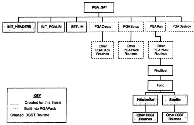
A-3-1 PGA_113_14 ... 266

A-3-2 SETLIM ... ... ... 269

A-3-3 FINDBEST ... 270

A-3-4 FUNC ... 271

A-4 113:14 REPEAT GROUND TRACK ELEMENT HISTORY PLOTS ... 275

A-4-1 113:14 Repeat Ground Track Zonal and Third Body Decay Plots ... 276

A-4-2 113:14 Repeat Ground Track Full Perturbation Decay Plots ... 278

APPENDIX B GEAR ARRAY DESIGN PROBLEM DATA ... 281

B- 1 GEAR ARRAY CONSTRAINT SURFACE PLOTS ... ... 281

B-I- APTS Constraint ... 282

B-1-2 Stroboscopic Constraint ... 284

B-1-3 Ratio Constraint ... 286

B-2 GEAR ARRAY PARAMETERIZATION OPTIONS SURFACE PLOTS ... 288

B-2- Offset Method ... 289

B-2-2 Fixed Circular Semi-Major Axis Method ... 291

B-2-3 Fixed Apogee Height Method ... 293

B-3 GEAR ARRAY OBJECTIVE FUNCTION CODE (FUNC) ... ... 295

B-4 GEAR ARRAY INPUT DECKS ... 299

B-4-1 Gear Array Circular Orbit DSST Input Deck ... ... 299

B-4-2 5:6 Gear Array APTS Elliptical Orbit DSST Input Deck . ... 301

B-5 GEAR ARRAY GENETIC ALGORITHM PERFORMANCE PLOTS ... 302

B-5-1 5:6 Gear 8050 km Apogee Case...303

B-5-2 4:5 Gear 0 km Offset Case ... 304

B-6 DESIRED GEAR BEHAVIOR AND ELEMENT DECAY PLOTS ... 305

B-6-1 5:6 Gear 8050 km Apogee Height Zonal 50 x 0 Field Decay Plots ... 306

B-6-2 5:6 Gear 8050 km Apogee Height Full Perturbation Decay Plots . ... 311

B-6-3 4:5 Gear 0 km Offset Zonal 50 x 0 Field Decay Plots ... 316

(16)

B-7 GEAR ARRAY COVERAGE ANALYSIS PLOTS ... ... 326

B-7-1 Local Time of Noon Coverage Analysis Plots ... 327

B-7-2 Local Time of 3:00 P.M. Coverage Analysis Plots ... 329

APPENDIX C GLOBAL STATION KEEPING APPROACH DATA ... 333

C- I CODE MODIFICATIONS FOR GLOBAL STATION KEEPING IMPLEMENTATION ... 333

C-1-1 FUNC ... 334

C- 1-2 DEFREFORB ... 340

C-1-3 CALCFIRSTDEVTIME ... 342

C-2 GLOBAL STATION KEEPING APPROACH DSST INPUT DECKS ... 343

C-2-1 Reference Orbit ... 344

C-2-2 Case I Actual Orbit ... 345

C-2-3 Case 2 Actual Orbit ... 347

C-3 GLOBAL STATION KEEPING CASE 1 ELEMENT DEVIATION PLOTS ... 348

C-3-1 Global Case 1 Uncontrolled Deviations ... 349

C-3-2 Global Case I Controlled Deviations ... 352

C-4 GLOBAL STATION KEEPING CASE 2 ELEMENT DEVIATION PLOTS ... 355

C-4-1 Global Case 2 Uncontrolled Deviations ... 356

C-4-2 Global Case 2 Controlled Deviations ... 359

APPENDIX D OPERATIONAL STATION KEEPING APPROACH DATA ... 363

D- I CODE MODIFICATIONS REQUIRED FOR OPERATIONAL APPROACH IMPLEMENTATION ... 363

D-J-1 Operational Approach Modifications to PGA_GASK ... 363

D-1-2 Operational Approach Modifications to FUNC ... 368

D-2 FEASIBILITY TEST OF THE OPERATIONAL APPROACH DEVIATION PLOTS ... 377

D-3 INPUT DECKS FOR OPERATIONAL APPROACH AS PLANNING TOOL . ... 381

D-3-1 Reference Orbit ... 381

D-3-2 Actual Orbit ... 382

(17)

D-4-1 Uncontrolled Deviation with Five-year Optimized Epoch Elements ... 384

D-4-2 Results of One Year Test of Operational Planning Tool ... 388

D-4-3 Results of 2.5 Year AV Estimation from Operational Planning Tool ... 392

D-4-4 1200 Day Optimization Using Operational Approach Results . ... 396

(18)

(19)

List of Figures

Figure 1-1 Ellipso Mobile Satellite System Orbits ... 36

Figure 2-1 Perturbing Acceleration Effects ... 44

Figure 2-2 Semi-Major Axis Depiction ... 47

Figure 2-3 Sample Eccentricities of the Four Conic Sections ... 47

Figure 2-4 The Geocentric-Equatorial Coordinate System ... 48

Figure 2-5 Four of the Keplerian Orbital Elements ... 49

Figure 2-6 Typical Hohmann Transfer ... 55

Figure 2-7 The Generalized Method of Averaging ... 63

Figure 3-1 Example of Greedy Optimization Strategy ... 89

Figure 3-2 Problem for Which Principle of Optimality can be Demonstrated . ... 91

Figure 3-3 Local vs. Global Optimal Point ... 94

Figure 3-4 Application of the Gauss-Seidel Method ... 95

Figure 3-5 Application of tle, Method of Steepest Descent ... 96

Figure 3-6 Application of Newton's Method ... 98

Figure 3-7 Gradient Method Convergence to Incorrect Solution ... 100

Figure 3-8 Cycle of Genetic Algorithm ... 103

Figure 3-9 Two-Point Crossover Operation ... ... 105

Figure 3-10 Mutation Operation ... 106

Figure 4-1 Program Structure for Powell's Method ... 120

Figure 4-2 113:14 Repeat Ground Track FUNC Overview ... 122

Figure 4-3 3-D Surface of 113:14 e/i Space (a = 10496.8968 km) ... ... 124

Figure 4-4 Contour Plot of 113:14 e/i Space (a = 10496.8968 kin) ... 125

Figure 4-5 Software Overview for 113:14 Genetic Algorithm Solution Process ... 127

Figure 4-6 String Structure for 113:14 Genetic Algorithm Optimization .... ... 130

Figure 4-7 Best 113:14 Objective Function Value vs. Iteration Number . ... 135

Figure 4-8 Average 113:14 Objective Function Value vs. Iteration Number ... 135

Figure 4-9 113:14 Repeat Ground Track Argument of Perigee Design Accuracy ... 137

(20)

Figure 4-10 113:14 Right Ascension of the Ascending Node Design Accuracy ... 138

Figure 4- 1 113:14 Argument of Perigee Decay Under Full Perturbations...140

Figure 4-12 113:14 RAAN Decay Under Full Perturbations ... 140

Figure 4-13 5:6 Gear Array Viewed from North Pole ... 142

Figure 4-14 APTS Constraint Behavior Contour Plot ... 145

Figure 4-15 Stroboscopic Constraint Behavior ... 148

Figure 4-16 Stroboscopic Constraint Behavior: Edge-on View ... 148

Figure 4-17 Ratio Constraint Behavior... 150

Figure 4-18 Offset Method Contour Plot ... 153

Figure 4-19 Fixed Circular Semi-Major Axis Method Contour Plot ... 153

Figure 4-20 Fixed Apogee Height Method Contour Plot ... 154

Figure 4-21 Gear Array Optimization FUNC Overview ... 156

Figure 4-22 5:6 Case Gear Design Genetic Algorithm Convergence Plot.. ... 159

Figure 4-23 4:5 Case Gear Design Genetic Algorithm Convergence Plot.. ... 160

Figure 4-24 4:5 Gear 0 km Offset 5-Year APTS SMA Divergence (Full Pert.) ... 166

Figure 4-25 Gear Array Minimum Elevation Angle Comparison-Noon Local Time ... 167

Figure 5-1 Box Constraint Depiction ... 170

Figure 5-2 Global Station Keeping Approach Genetic Algorithm String Structure ... 175

Figure 5-3 Global Station Keeping Genetic Algorithm Software Overview ... 184

Figure 5-4 Global Station Keeping Optimization FUNC Routine Overview ... 186

Figure 5-5 Global Case 1 Uncontrolled Mean Anomaly Drift (Limit = 1 °) ... 191

Figure 5-6 Global Case 2 Uncontrolled Argument of Perigee Drift (Limit = 1 °) ... 192

Figure 5-7 Global Case 2 Uncontrolled Mean Anomaly Drift (Limit = 1° )... 193

Figure 5-8 Global Case I Controlled Eccentricity Deviation (Limit = 0.0003) . ... 195

Figure 5-9 Global Case 1 Controlled Mean Anomaly Deviation (Limit = 1 °) ... 196

Figure 5-10 Global Case 2 Controlled Argument of Perigee Deviation (Limit = 1 ) ... 198

Figure 5-11 Global Case 2 Controlled Mean Anomaly Deviation (Limit = 1 )... 198

(21)

Figure 5-13 Semi-Major Axis History for Controlling Argument of Perigee with Radial and Tangeatial

Burns ... 201

Figure 5-14 Operational GA Optimization Approach Overview ... 216

Figure 5-15 Operational Feasibility Test Controlled Mean Anomaly Deviation (Limit = 1 ) ... 221

Figure 5-16 Operational Feasibility Test Controlled Argument of Perigee Deviation (Limit = 1 °) ... 222

Figure 5-17 One Year Operational Approach Planning Test Semi-major Axis Deviation (Limit = 1 km) 229 Figure 5-18 One Year Operational Approach Planning Test Eccentricity Deviation (Limit = 3x 04) ... 229

Figure 5-19 2.5-Year Operational Planning Approach Semi-Major Axis Deviation (Limit = km) ... 232

Figure 5-20 2.5-Year Operational Planning Approach RAAN Deviation (Limit = 0.5° ) ... 234

Figure 5-21 RAAN Deviation of 1200 Day Optimization Showing Greedy Behavior ... 236

Figure 5-22 Cumulative Delta-V vs. Time for Greedy Case ... 238

Figure 5-23 Number of Burns Required vs. Time for Greedy Case ... 238

Figure A-1 3-D Surface of 113:14 a/e Space (i = 116.5782 )... 260

Figure A-2 Contour Plot of 113:14 a/e Space (i = 116.5782 )... 260

Figure A-3 Eccentricity Edge-on View of 113:14 a/e Space (i = 116.5782 °)... 261

Figure A-4 Semi-Major Axis Edge-on View of 113:14 a/e Space (i = 116.57820)... 261

Figure A-5 3-D Surface of 113:14 e/i space (a = 10496.8968 km) ... 262

Figure A-6 Contour Plot of 113:14 e/i space (a = 10496.8968 km) ... 262

Figure A-7 Eccentricity Edge-On View of 113:14 e/i space (a = 10496.8968 km) ... 263

Figure A-8 Inclination Edge-On View of 113:14 e/i space (a = 10496.8968 km) ... 263

Figure A-9 3-D Surface of 113:14 a/i Space (e = 0.32986) ... ... 264

Figure A-10 Contour Plot of 113:14 a/i Space (e = 0.32986) ... 264

Figure A-Il Semi-major Axis Edge-on View of 113:14 a/i Space (e = 0.32986) ... 265

Figure A-12 Inclination Edge-on View of 113:14 a/i Space (e = 0.32986) ... 265

Figure A-13 113:14 SMA Deviation from 10496.8968 km (Zonals/3B Pert.) ... 276

Figure A-14 113:14 Eccentricity Deviation from 0.32986 (Zonals/3B Pert.) .. ... 276

Figure A-15 113:14 Inclination Deviation from 116.5782° (Zonals/3B Pert.) ... 277

Figure A-16 113:14 Node Deviation from Calculated Values (Zonals/3B Pert.) ... 277 21

(22)

Figure A-17 113:14 Perigee Deviation from 260° (Zonals/3B Pert.) ... 278 Figure A-18 113:14 Semi-Major Axis Deviation from 10496.8968 km (Full Pert.) ... 278 Figure A-19 113:14 Eccentricity Deviation from 0.32986 (Full Pert.) ... 279 Figure A-20 113:14 Inclination Deviation from 116.5782°(Full Pert.) ... 279 Figure A-21 113:14 Node Deviation from Calculated Values (Full Pert.) ... 280 Figure A-22 113:14 Perigee Deviation from 260°(Full Pert.) ... 280

Figure B- 1 3-D View of APTS Constraint Surface ... 282 Figure B-2 Contour Plot of APTS Constraint Surface ... 282 Figure B-3 Semi-Major Axis Edge on View of APTS Constraint Surface ... 283 Figure B-4 Eccentricity Edge-on View of APTS Constraint Surface ... 283 Figure B-5 3-D View of Stroboscopic Constraint Surface ... 284 Figure B-6 Contour Plot of Stroboscopic Constraint Surface ... 284 Figure B-7 Semi-Major Axis Edge-on View of Stroboscopic Constraint Surface... 285 Figure B-8 Eccentricity Edge-on View of Stroboscopic Constraint Surface ... 285 Figure B-9 3-D View of Ratio Constraint Surface ... 286 Figure B-10 Contour Plot of Ratio Constraint Surface ... 286 Figure B- 11 Semi-Major Axis Edge-on View of Ratio Constraint Surface . ... 287 Figure B-12 Eccentricity Edge-on View of Ratio Constraint Surface ... 287 Figure B-13 3-D View of Offset Method Parameterization Surface ... 289 Figure B-14 Contour Plot of Offset Method Parameterization Surface ... 289 Figure B-15 Semi-Major Axis Edge-on View of Offset Method Parameterization ... 290 Figure B-16 Eccentricity Edge-on View of Offset Method Parameterization Surface ... 290 Figure B-17 3-D View of Fixed Circular SMA Parameterization Surface ... 291 Figure B-18 Contour Plot of Fixed Circular SMA Parameterization Surface . ... 291 Figure B- 19 SMA Edge-on View of Fixed Circular SMA Parameterization ... 292 Figure B-20 Eccentricity Edge-On View of Fixed Circular SMA Parameterization ... 292 Figure B-21 3-D View of Fixed Apogee Height Parameterization Surface ... 293 Figure B-22 Contour Plot of Fixed Apogee Height Parameterization Surface ... 293

(23)

Figure B-23 Circular SMA Edge-on View of Fixed Apogee Height Parameterization ... 294 Figure B-24 Eccentric SMA Edge-on View of Fixed Apogee Height Parameterization Surface ... 294 Figure B-25 Best 5:6 Gear Array Objective Function Value Convergence ... 303 Figure B-26 Average 5:6 Gear Array Objective Function Value Convergence . ... 303 Figure B-27 Best 4:5 Gear Array Objective Function Value Convergence ... 304 Figure B-28 Average 4:5 Gear Array Objective Function Value Convergence . ... 304 Figure B-29 5:6 Gear APTS Constraint Error (Zonals Only) ... 306 Figure B-30 5:6 Gear Stroboscopic Constraint Error (Zonals Only) ... 306 Figure B-31 5:6 Gear Ratio Constraint Error (Zonals Only) ... 307 Figure B-32 5:6 Gear APTS Semi-major Axis Deviation from 12527.3713 km (Zonals Only) ... 307 Figure B-33 5:6 Gear APTS Eccentricity Deviation from 0.15172 (Zonals Only) ... 308 Figure B-34 5:6 Gear APTS Inclination Deviation from 0.0°(Zonals Only) ... 308 Figure B-35 5:6 Gear APTS Mean Anomaly History (Zonals Only) ... 309 Figure B-36 5:6 Gear Circular Semi-major Axis Deviation from 14143.57 km (Zonals Only) ... 309 Figure B-37 5:6 Gear Circular Eccentricity Deviation from 0.0 (Zonals Only) ... 310 Figure B-38 5:6 Gear Circular Inclination Deviation from 0.0° _{(Zonals Only) ...}

310 Figure B-39 5:6 Gear APTS Constraint Error (Full Pert.) ... 311 Figure B-40 5:6 Gear Stroboscopic Constraint Error (Full Pert.) ... 311 Figure B-41 5:6 Gear Ratio Constraint Error (Full Pert.) ... 312 Figure B-42 5:6 Gear APTS Semi-major Axis Deviation from 12527.3713 km (Full Pert.) ... 312 Figure B-43 5:6 Gear APTS Eccentricity Deviation from 0.15172 (Full Pert.) ... 313 Figure B-44 5:6 Gear APTS Inclination Deviation from 0.0° (Full Pert.) ... 313 Figure B-45 5:6 Gear APTS Mean Anomaly History (Full Pert.) ... 314 Figure B-46 5:6 Gear Circular Semi-major Axis Deviation from 14143.57 km (Full Pert.) ... 314 Figure B-47 5:6 Gear Circular Eccentricity Deviation from 0.0 (Full Pert.) ... 315 Figure B-48 5:6 Gear Circular Inclination Deviation from 0.0°_{(Full Pert.) .} _...

315 Figure B-49 4:5 Gear APTS Constraint Error (Zonals Only) ... 316 Figure B-50 4:5 Gear Stroboscopic Constraint Error (Zonals Only) ... 316

(24)

Figure B-51 4:5 Gear Ratio Constraint Error (Zonals Only) ... 317 Figure B-52 4:5 Gear APTS Semi-major Axis Deviation from 12546.5718 km (Zonals Only) ... 317 Figure B-53 4:5 Gear APTS Eccentricity Deviation from 0.16011 (Zonals Only) ... 318 Figure B-54 4:5 Gear APTS Inclination Deviation from 0.0° (Zonals Only) ... 318 Figure B-55 4:5 Gear APTS Mean Anomaly History (Zonals Only) ... 319. Figure B-56 4:5 Gear Circular Semi-Major Axis Deviation from 14555.4545 km (Zonals Only) ... 319 Figure B-57 4:5 Gear Circular Eccentricity Deviation from 0.0 (Zonals Only) ... 320 Figure B-58 4:5 Gear Circular Inclination Deviation from 0.0° (Zonals Only) ... 320 Figure B-59 4:5 Gear APTS Constraint Error (Full Pert.) ... 321 Figure B-60 4:5 Gear Stroboscopic Constraint Error (Full Pert.) ... 321

Figure B-61 4:5 Gear Ratio Constraint Error (Full Pert.) ... 3... 322 Figure B-62 4:5 Gear APTS Semi-Major Axis Deviation from 12546.5718 km (Full Pert.) ... 322

Figure B-63 4:5 Gear APTS Eccentricity Deviation from 0.16011 (Full Pert.) ... 323 Figure B-64 4:5 Gear APTS Inclination Deviation from 0.0 (!! Pert.) ... 323 Figure B-65 4:5 Gear APTS Mean Anomaly History (Full Pert.) ... 324 Figure B-66 4:5 Gear Circular Semi-Major Axis Deviation from 14555.4545 km (Full Pert.) ... 324 Figure B-67 4:5 Gear Circular Eccentricity Deviation from 0.0 (Full Pert.) ... 325 Figure B-68 4:5 Gear Circular Inclination Deviation from 0.0° (Full Pert.) . ... 325 Figure B-69 Minimum Elevation Angle Comparison-Noon Local Time . ... 327 Figure B-70 Average Elevation Comparison-Noon Local Time ... 327 Figure B-71 Minimum Number of Satellites in View Comparison-Noon Local Time ... 328 Figure B-72 Maximum Number of Satellites in View Comparison-Noon Local Time ... 328 Figure B-73 Average Number of Satellites in View Comparison-Noon Local Time ... 329 Figure B-74 Minimum Elevation Comparison-3 P.M. Local Time ... 329 Figure B-75 Average Elevation Comparison-3 P.M. Local Time ... 330 Figure B-76 Minimum Number of Satellites in View Comparison-3 P.M. Local Time ... 330 Figure B-77 Maximum Number of Satellites in View Comparison-3 P.M. Local Time ... 331 Figure B-78 Average Number of Satellites in View Comparison-3 P.M. Local Time ... 331

(25)

Figure C- Global Case 1 Uncontrolled SMA Deviation (Limit = o) ... 349 Figure C-2 Global Case 1 Uncontrolled Eccentricity Deviation (Limit = 0.0003) ... 349 Figure C-3 Global Case 1 Uncontrolled Inclination Deviation (Limit = 0.05)... 350 Figure C-4 Global Case Uncontrolled RAAN Deviation (Limit = 0.5 )... 350 Figure C-5 Global Case 1 Uncontrolled Argument of Perigee Deviation (Limit = 1 ) ... 351 Figure C-6 Global Case 1 Uncontrolled Mean Anomaly Deviation (Limit = 1 ) ... 351 Figure C-7 Global Case 1 Controlled SMA Deviation (Limit = 1 km).. ... 352 Figure C-8 Global Case 1 Controlled Eccentricity Deviation (Limit = 0.0003) ... 352 Figure C-9 Global Case 1 Controlled Inclination Deviation (Limit = 0.05 )... 353 Figure C-10 Global Case 1 Controlled RAAN Deviation (Limit = 0.5 ) ... 353 Figure C- 11 Global Case 1 Controlled Argument of Perigee Deviation (Limit = 1 ) ... 354 Figure C-12 Global Case 1 Controlled Mean Anomaly Deviation (Limit = 1 ) ... 354 Figure C- 13 Global Case 2 Uncontrolled SMA Deviation (Limit = I kmin). ... 356 Figure C-14 Global Case 2 Uncontrolled Eccentricity Deviation (Limit = 0.0003) ... 356 Figure C-15 Global Case 2 Uncontrolled Inclination Deviation (Limit = 0.05°) ... 357 Figure C-16 Global Case 2 Uncontrolled RAAN Deviation (Limit = 0.5) ... 357 Figure C- 17 Global Case 2 Uncontrolled Argument of Perigee Deviation (Limit = 1° )... 358 Figure C-18 Global Case 2 Uncontrolled Mean Anomaly Deviation (Limit = 1° )... 358 Figure C-19 Global Case 2 Controlled SMA Deviation (Limit = 1 km).. ... 359 Figure C-20 Global Case 2 Controlled Eccentricity Deviation (Limit = 0.0003) ... 359 Figure C-21 Global Case 2 Controlled Inclination Deviation (Limit = 0.05 )... 360 Figure C-22 Global Case 2 Controlled RAAN Deviation (Limit = 0.5)... 360 Figure C-23 Global Case 2 Controlled Argument of Perigee Deviation (Limit = 1 ) ... 361 Figure C-24 Global Case 2 Controlled Mean Anomaly Deviation (Limit = 1)... 361

Figure D- 1 Operational Feasibility Test SMA Deviation (Limit = 1 km) ... 378 Figure D-2 Operational Feasibility Test Eccentricity Deviation (Limit = 0.0003) ... 378 Figure D-3 Operational Feasibility Test Inclination Deviation (Limit = 0.05 )... 379

(26)

Figure D-4 Operational Feasibility Test RAAN Deviation (Limit = 0.5 )... 379 Figure D-5 Operational Feasibility Test Arg. of Perigee Deviation (Limit = 1° )... 380 Figure D-6 Operational Feasibility Test Mean Anormraly Deviation (Limit = 1 ) ... 380 Figure D-7 Operational Planning Case Uncontrolled SMA Deviation (Limit = 1 km) ... 385 Figure D-8 Operational Planning Case Uncontrolled e Deviation (Limit = 0.0003) ... 385 Figure D-9 Operational Planning Case Uncontrolled i Deviation (Limit = 0.05° ) ... 386 Figure D-10 Operational Planning Case Uncontrolled Q Deviation (Limit = 0.5°)... 386 Figure D- 11 Operational Planning Case Uncontrolled o Deviation (Limit = 1) ... 387 Figure D- 12 Operational Planning Case Uncontrolled M Deviation (Limit = 1° )... 387 Figure D-13 1-Year Operational Planning Approach SMA Deviation (Limit = 1 km) ... 389 Figure D-14 1-Year Operational Planning Approach e Deviation (Limit = 0.0003) ... 389 Figure D-15 -Year Operational Planning Approach i Deviation (Limit = 0.05°)... 390 Figure D-16 1-Year Operational Planning Approach K2 Deviation (Limit = 0.5° )... 390 Figure D-17 1-Year Operational Planning Approach co Deviation (Limit = 1 )... 391 Figure D- 18 1-Year Operational Planning Approach M Deviation (Limit = 1 ) ... 391 Figure D- 19 2.5-Year Operational Planning Case SMA Deviation (Limit = 1 km) ... 393 Figure D-20 2.5-Year Operational Planning Case e Deviation (Limit = 0.0003) ... 393 Figure D-21 2.5-Year Operational Planning Case i Deviation (Limit = 0.05° )... 394 Figure D-22 2.5-Year Operational Planning Case Q Deviation (Limit = 0.5 )... 394 Figure D-23 2.5-Year Operational Planning Case o Deviation (Limit = 1 ) ... 395 Figure D-24 2.5-Year Operational Planning Case M Deviation (Limit = 1 ) ... 395 Figure D-25 1200 Day Operational Planning Case SMA Deviation (Limit = 1 km) ... 397 Figure D-26 1200 Day Operational Planning Case e Deviation (Limit = 0.0003)... 397 Figure D-27 1200 Day Operational Planning Case i Deviation (Limit = 0.05)... 398 Figure D-28 1200 Day Operational Planning Case Q Deviation (Limit = 0.50)... 398 Figure D-29 1200 Day Operational Planning Case co Deviation (Limit = 1) ... 399 Figure D-30 1200 Day Operational Planning Case M Deviation (Limit = 10) ... 399

(27)

List of Tables

Table 1-1 Principal Mission Requirements and Design Parameters ... 30 Table 1-2 Comparisons of Pers .nal Communications Satellite Systems ... 35 Table 3-1 Variable and Condition Summary for Optimal Control Problems . ... 84 Table 4-1 113:14 Results from Powell's Method Optimization ... 126 Table 4-2 113:14 Case Genetic Algorithm Parameters ... 134 Table 4-3 GA Derived Optimal Elements for the Borealis Node at Noon 113:14 Case ... 136 Table 4-4 Borealis Node at Noon 113:14 Design Accuracy over 5 Year Life Span ... 138 Table 4-5 BorealisTM Node-at-Noon 113:14 Design Decay over 5 Year Life Span under Full Perturbations

... .141 Table 4-6 Gear Array Genetic Algorithm Parameters ... 158 Table 4-7 Optimal Gear Array Design Parameters ... ... 161 Table 4-8 5:6 Gear 8050 Apogee Design Accuracy ... ... 162 Table 4-9 4:5 Gear 0 km Offset Design Accuracy ... 163 Table 4-10 5:6 Gear 8050 Apogee Decay Under Full Perturbations ... 164 Table 4-11 4:5 Gear 0 km Offset Decay Under Full Perturbations ... 164 Table 5-1 GA Global Station Keeping Solution Process Variable Allocation . ... 176 Table 5-2 Global Station Keeping Approach Genetic Algorithm Parameters ... 178 Table 5-3 90-Day Optimized Ellipso BorealisT Node at Noon Epoch Elements and Tolerances ... 189 Table 5-4 Global Case 1 Epoch Elements and Uncontrolled Deviations ... 190 Table 5-5 Global Case 2 Epoch Elements And Uncontrolled Deviations ... 192 Table 5-6 Global Case 1 Burn Times and Components ... 194 Table 5-7 Global Case 2 Burn Times and Components ... 197 Table 5-8 Global Station Keeping GA and ASKS Results Comparison ... 203 Table 5-9 Global vs. Operational Optimization Approach Comparison ... 212 Table 5-10 GA Operational Station Keeping Solution Process Variable Allocation ... 213 Table 5-11 Operational Station Keeping Approach Maximum Drift Time Optimization Genetic Algorithm

(28)

Table 5-12 Operational Station Keeping Approach AV Optimization Genetic Algorithm Parameters ... 217 Table 5-13 Operational Approach Feasibility Test Case Burn Times and Components ... 220 Table 5-14 5-Year Optimized Ellipso BorealisT M _{Node at Noon Epoch Elements and Tolerances ... 226}

Table 5-15 2.5-Year Borealis Node-at-Noon AV Planning Test Results ... 231 Table 6-1 Optimal Epoch Elements for the Borealis Node at Noon 113:14 5-Year Optimization

(Epoch = January 1, 1997) ... ... 245 Table 6-2 Optimal Gear Array Design Parameters ... 247 Table 6-3 90-Day Optimized Ellipso BorealisTM Node at Noon Epoch Elements and Tolerances

(Epoch = March 21, 2000) ... ... 250 Table 6-4 Results of Two Global Station Keeping Optimization Test Cases ... 250 Table 6-5 Genetic Algorithm Parameter Comparison ... 251 Table 6-6 Results of Three Operational Station Keeping AV Planning Test Cases ... 255

(29)

Chapter 1 Introduction

1-1 Statement of Objectives

In the field of astrodynamics, the areas of orbit design and on-orbit maintenance can have a significant impact upon the success of a given mission. Placing a satellite into an improperly designed orbit can greatly reduce the effectiveness of that satellite in accomplishing its given mission objectives. Similarly, an inability to maintain a spacecraft in the properly designed orbit can also have disastrous effects on the mission of that satellite.

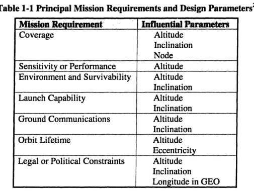
All satellite orbit design is accomplished by first establishing orbit-related mission requirements. Requirement definition is the first step in orbit design as the choice of orbit typically defines not only the satellite's location in space, but also a number of other factors including the space mission lifetime, cost, environment, viewing geometry, and often also payload performance'. Table 1-1 lists a number of mission requirements along with parameters that can have an affect on these mission requirements. Due to the significant effect that the orbit design has on each of these mission requirement related aspects, finding the best or optimal design deserves special attention. By placing emphasis on finding the optimal orbit design, satellite designers can obtain corresponding gains in the overall mission performance of a spacecraft.

' Larson, Wiley J. and James R. Wertz. Space Mission Analysis and Design, Torrance, California: Microcosm, Inc., 1992, p. 157.

(30)

Table 1-1 Principal Mission Requirements and Design Parameters2

Mission Requirement' Influential Parameters

Coverage Altitude

Inclination Node

Sensitivity or Performance Altitude

Environment and Survivability Altitude Inclination

Launch Capability Altitude

Inclination

Ground Communications Altitude

Inclination

Orbit Lifetime Altitude

Eccentricity Legal or Political Constraints Altitude

Inclination

Longitude in GEO

In addition to design of the optimal orbit, finding optimal methods for performing satellite orbit maintenance or "station-keeping" also deserves added emphasis. Even with an optimally designed orbit, if that orbit and/or station within that orbit are not maintained, the performance of the satellite will degrade. Additionally, due to recent gains in the operational lifetime of a variety of satellite component technologies, satellites can maintain on-orbit operational capabilities for longer periods of time than previously estimated. Despite these gains in the operational lifetime of the component technologies, if the spacecraft cannot be maintained in the necessary orbit, there will be no corresponding gain in the operational lifetime of the satellite. Therefore, on-board fuel limitations have an increasingly important role in determining the overall lifetime of spacecraft. By finding optimal station keeping strategies, designers can not only decrease

2 Larson, Wiley J. and James R. Wertz. Space Mission Analysis and Design, Torrance, California: Microcosm, Inc., 1992, p. 179.

(31)

the amount of required on-board fuel, but potentially increase both the satellite lifetime and corresponding system effectiveness metric as well.

The broad objective of this thesis is to explore ways in which both traditional and non-traditional optimization methods can be applied to find improvements in these two mission critical areas of satellite orbit design and on-orbit maintenance. Specifically, this thesis is a compilation of efforts to discover both orbit designs and station-keeping strategies capable of increasing the mission performance of multi-satellite constellations.

1-2 Optimization

Inherent to the efforts of this thesis is the concept of optimization. This concept of optimization can be defined in a number of ways. The American Heritage Dictionary3 states that to optimize something is "to make the most effective use of' it. In many mathematical or other applications, this definition is applied very literally, and finding optimal solutions means obtaining the absolutely best solutions to a given problem. This interpretation is the conventional view of optimization as explained by Beightler, Phillips, and Wilde4:

Man's longing for perfection finds expression in the theory of optimization. It studies how to describe and attain what is Best, once one knows how to measure and alter what is Good or Bad.... Optimization theory encompasses the quantitative study of optima and methods for finding them.

3 The American Heritage Dictionary of the English Language, Houghton Mifflin Company, Boston, Massachusetts, 1981.

4 Beightler, C. S., D. T. Phillips, and D. J. Wilde. Foundations of Optimization, Englewood Cliffs, New Jersey: Prentice-Hall, 1979, p. 1.

(32)

Although finding what is "Best" is the conventional view of optimization, it is not necessarily the only or natural definition. In human decision making, decisions are not usually made based on what is the perfect decision, as this "Best" solution is not typically available. Rather, human decision-makers take into account many factors and choose the solution that, at the time, appears better than any other available options. This more humanized view of optimization is a more natural definition and appears in many applications. In these applications, the goal of optimization shifts, from finding the best solution, to simply finding improvement.5 Using this definition, optimal solutions are not those that give perfect performance, but instead are those that give better performance relative to other solutions. This concept of attempting to quickly find some good level of performance is known as "satisficing"6 and is the view of optimization taken most frequently throughout this work.

1-3 Satellite Constellations

A recent trend in commercial satellite design has been the application of more than one satellite to a given mission. Due to the coordinated manner in which these satellites must perform in order to meet overall mission objectives, these multiple satellites are termed constellations. There are advantages which are evident when more than one satellite is applied to a given mission, but also a number of areas to which precise solutions (and hence optimization) becomes more important.

The main advantage gained when multiple space vehicles are applied to the same mission is in terms of coverage, or areas of the Earth that can see a satellite at any given

5 Goldberg, David E. Genetic Algorithms in Search, Optimization, and Machine Learning, Reading, Massachusetts: Addison-Wesley Publishing Company, Inc., 1989, p. 7.

(33)

time. With one satellite it is impossible to have coverage of more than one area of the globe at a given time. For most satellites, only a certain area of the Earth is covered and this area moves as the satellite orbits the Earth. However, if an appropriate number of satellites are placed in designated locations around the Earth, larger and larger portions of the Earth can be covered. In the late 1960s, Easton and Brecia of the United States Naval Research Laboratory in their 1969 report Continuously Visible Satellite Constellations analyzed coverage by satellites in two mutually perpendicular orbit planes and concluded that at least six satellites would be needed to provide full global coverage.7 In the 1970s, J.G. Walker considered orbit types not previously considered by Easton and Brecia and concluded that continuous coverage of the Earth would require only five satellites8. Following this trend, John Draim, in the 1980s found and patented a constellation of four satellites in elliptical orbits that provide continuous Earth coverage.9

Achieving greater coverage through constellations is not without cost, however. Most noticeable of these costs is the cost to build additional satellites. In order to have multiple satellites in space, multiple satellites must first be built and launched at great expense. Improper design of satellite orbits which calls for a greater number of satellites than is actually needed can have a direct impact on a program's cost. Therefore, optimization is a useful tool in the design of these multi-satellite constellations.

The maintenance of multi-satellite constellations is also an area in which application of proper optimization techniques can lead to program cost savings. An

6 Simon, H. A. The Sciences of the Artificial, Cambridge, Massachusetts: MIT Press, 1969.

7. Larson, Wiley J. and James R. Wertz. Space Mission Analysis and Design, Torrance, California: Microcosm, Inc., 1992, p. 189.

8 Walker, J. G. "Satellite Constellations," Journal of the British Interplanetary Society. 1984, 37: 559-572.

(34)

optimally designed orbit is of little use if the satellite cannot be maintained in that orbit. An unfortunate fact of astrodynamics is that the orbits of satellites degrade. Therefore, in order to achieve mission objectives, small correctional maneuvers must often be performed such that the satellite is repositioned into the desired orbit. Each of these maneuvers, however, has an associated fuel cost. Through application of optimization techniques, the minimum fuel maneuvers can be found which allow the satellite to maintain the designed orbit and therefore, achieve the desired mission objectives at minimum cost. For constellations where the orbits of multiple satellites must be maintained and orbital maintenance costs are multiplied by the number of satellites, finding the minimum fuel maneuvers becomes even more of a priority.

1-3-1 Communication Constellations

An important mission to which constellations have been applied recently is the area of communications, specifically mobile communications. The gains in coverage through the application of multiple satellites to one mission are especially advantageous to the achievement of a communications mission. The goal of this type of mission is simple: provide a means whereby a user in one location on the globe can communicate with a user at an entirely different location on the globe. With only one satellite, achievement of this goal is impossible. However, by careful design and placement of the satellites in a constellation, coverage is increased and the goal of global mobile communications can become a reality.

9 Draim, John. "Three- and Four-Satellite Continuous Coverage Constellations," Journal of Guidance, Control, and Dynamics, 1985, 6: 725-730.

(35)

Seeing the advantage that constellations present to the achievement of a communications mission, a number of companies have proposed systems to meet this goal. At the present time, one of these companies (Iridium) has succeed in creating an operating systemT

' while the others are scheduled to begin operation within the next few years. The specific details about these constellations can be seen in Table 1-2. Note that the data presented in this table is only an approximation as precise orbital designs are often considered proprietary information.

Table 1-2 Comparisons of Personal Communications Satellite Systems"

Orbit Type Altitude (km) Eccentricity Inclination (deg) Period (hr) Number of Sats Number of Planes

Number of Sats Per Plane

Ellipso Borealis/Concordia SSFLA 520-7846 / 8063 0.33 /0.0 116.6/0.0 3.0/4.67 10/8 2/1 5/8 Globalstar'2 LEO 1414 0.0 52.0 1.9 48 8 6

Iridium13 ICO14 Teledesic'

LEO 780 0.0013 86.4 MEO 10390 LEO 1375 0.0 0.00118 45.0 1.7 6.0 66 6 11 10 2 5 98.2 1.9 288 12 24 NOTE: This table contains values that are more up to date than those available in the original reference. The more up to date values were taken from the home pages of the individual companies as contained in the footnotes.

Io Swan, Peter A. "Iridium Gets Re;al," Aerospace America, Vol. 37, No. 2, February 1999, p. 23.

1 Hulkover, Neal D., A Reevaluation of Ellipso Tr Globalstar, IRIDIUM TMand Odyssey ™, Presentation at

Volpe Transportation Center, Cambridge, Massachusetts, 18 October 1994.

12 Globalstar Corporation Internet Homepage. Available at www.globalstar.com. Accessed 28 April 1999. 13 Iridium Corporation Internet Homepage. Available at www.iridium.com. Accessed 28 April 1999. 14 _{ICO Internet Homepage. Available at www.ico.com. Accessed 28 April 1999.}

15 Teledesic Internet Homepage. Available at www.teledesic.com. Accessed 28 April 1999.

(36)

1-3-2 EllipsoTM Constellation

For all of the studies found in this thesis, the EllipsoTM _{constellation was used for}

analysis. As seen in Table 1-2, most of the designs for communications constellations are based on circular orbits. The only constellation that deviates from this circular standard is the EllipsoTM _{constellation.} _{Although the optimization techniques discussed and}

implemented throughout this thesis would be applicable to the circular cases, as well, the non-circular nature of the EllipsoTM constellation presented a slightly more challenging case to which to apply and test the techniques.

Figure 1-1 Ellipso Mobile Satellite System Orbits16

Figure 1-1 depicts the design of the EllipsoTM _{communications constellation}

designed by Ellipso, Inc. This constellation achieves near global coverage using two low/medium altitude sub-constellations operating in tandem. The concept of two

16 Castiel, D. J. W. Brosius, and J. E. Draim. Ellipso T Coverage Optimization Using Elliptic Orbits,

Paper AIAA-94-1098-CP, 15'h AIAA International Communications Satellite Systems Conference, San Diego, California, 28 February to 3 March 1994.

(37)

low/medium altitude sub-constellations operating in tandem, developed and patented by Castiel, Draim, and Brosius'7_{, is more efficient than traditional constellation designs in} balancing the dual demands of global coverage and transmission power.18

The first of the two EllipsoTM sub-constellations is known as BorealisT M_.

BorealisT M _{consists of two critically inclined, sun-synchronous eccentric orbit planes with}

a frozen line of apsides (SSFLA). These two orbit planes are aligned 180° apart, with one ascending node at noon and the other at midnight. This configuration provides 24-hour coverage of the Northern Hemisphere with four spacecraft and one on-orbit spare in each orbital plane.

BorealisTM_{is complemented by a second sub-constellation-a circular, equatorial}

sub-constellation known as ConcordiaT M_. _ConcordiaTM _{is a medium-altitude circular} equatorial orbit consisting of seven satellites and one on-orbit spare. It provides coverage around the tropical and southern latitudes. The altitude of the ConcordiaTM sub-constellation is approximately equal to the apogee height of the BorealisTM

sub-constellation to insure that the same communications equipment can be used for all satellites in the constellation.

1-4 Thesis Overview

The remainder of this thesis is divided into two main sections: a discussion of the techniques and technologies that allow for optimization to be applied to constellation

1_{7 Castiel, D., J. E. Draim and J. W. Brosius. Elliptical Orbit Satellite System and Deployment with}

Controllable Coverage Characteristics, United States Patent Number 5,582,367, 10 December 1996.

18 Draim, J. E. and T. J. Kacena. Populating the Abyss-Investigating More Efficient Orbits, Proceedings

of 6hAnnual AIAA/USU Conference on Small Satellites, Utah State University, Logan, Utah, 21-24 September 1992.

(38)

design and a discussion of the specific cases to which these optimization techniques were applied. Chapters 2 and 3 fall into the first section. Chapter 2 describes the basic enabling technologies and fundamentals required for performing orbit design. Specifically, orbit basics, orbit propagation, and computer aspects of orbit propagation are discussed. This discussion of astrodynamic fundamentals is followed by Chapter 3 in which specific optimization techniques and algorithms are presented. Chapters 4 and 5 discuss the application of these optimization techniques to the orbit design and maintenance applications. Chapter 4 presents an overview of the element/orbit design to which these optimization techniques were applied while Chapter 5 presents an application of the optimization techniques to a specific aspect of satellite constellation maintenance-station-keeping. Finally, Chapter 6 contains some observations resulting from the work completed for this thesis as well as some recommendations for future work.

(39)

Chapter 2 Enabling Techniques and Theories

As this thesis is based upon optimization of various applications relating to satellite constellations, a basic understanding of satellite motion (i.e. astrodynamics) is first required. Although it is impossible to explain astrodynamics in a single chapter, this chapter is an attempt to give the reader who is unschooled in astrodynamics a brief introduction to the basic concepts of this discipline. Specifically, the fundamental concepts used to describe a satellite's orbit and its motion along that orbit are briefly discussed. In an effort to provide a basis for the constellation maintenance applications, basic burn strategies are then presented. An explanation of satellite propagation techniques, and the use of parallel processing in satellite propagation applications, follows this description.

2-1 Fundamentals of Astrod ynamics

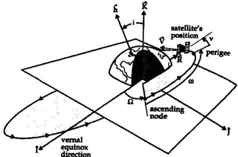
The motion of bodies in space has been studied for centuries. As early as 300 BC Aristotle had developed a complex, mechanical model of the universe. Others, including Ptolemy, Copernicus, Brahe, Kepler, and Galileo added to his contributions.'9 These men, along with many others, helped to lay the foundation of modern astrodynamics, and astrodynamics, in turn, is necessary to lay the foundation for this work.

In order to apply optimization techniques to various satellite constellation applications, it first becomes necessary to understand how objects move in space and also

19 Sellers, Jerry Jon. Understanding Space: An Introduction to Astronautics, New York, New York: McGraw-Hill, Inc., 1994, p. 32.

(40)

to understand the conventions used to describe an orbit and to differentiate one orbit from another. This section is intended to impart some of that understanding to the reader. The discussions in this section are the author's compilation from the following excellent astrodynamic references:

I. Fundamentals of Astrodynamics. By Roger R. Bate, Donald D. Mueller, and

Jerry E. White.20

II. An Introduction to the Mathematics and Methods of Astrodynamics. By Richard H. Battin.2'

III. Understanding Space: An Introduction to Astronautics. By Jerry Jon Sellers.22

IV. Fundamentals of Astrodynamics and Applications. By David A. Vallado.2 3 The interested reader is directed to these sources for a more in depth discussion of any of the fundamental concepts discussed here.

2-1-1 Orbital Motion

Like all motion, the basis for orbital motion is found in Newton's three laws. Especially of interest in astrodynamics is Newton's second law that states that the time rate of change of an object's momentum is equal to the applied force.24 For objects of constant mass, this law is often summarized as follows:

20 New York, New York: Dover Publications, Inc, 1971.

21 New York, New York: American Institute of Aeronautics and Astronautics, 1987.

22 New York, New York: McGraw-Hill, Inc, 1994. 23 New York, New York: McGraw-Hill, Inc, 1997.

24 Sellers, Jerry Jon. Understanding Space: An Introduction to Astronautics, New York, New York:

McGraw-Hill, Inc., 1994, p. 105.

(41)

F = m. * Equation 2-1 where:

F = applied force vectors

m = mass of the body

a = acceleration vector

By enumeration of the forces that act on a satellite orbiting the Earth, a general understanding of orbit motion can begin to be developed. Some of these forces include:

• The gravitational force of the Earth * Drag from the upper atmosphere

· Third-Body gravitational effects from the Sun, the Moon, or other non-Earth bodies

* Solar radiation pressure * Thrust from on-board rockets

By including these and other forces acting on a body in motion about the earth in Equation 2-1, the corresponding acceleration of a body can be computed and the motion of the satellite can then be described (this is the basis of the orbit propagation, see section 2-3). However, to gain an initial understanding of the type of motion to be expected, a number of simplifying assumptions, leading to the creation of the restricted two-body problem, are usually made.

(42)

2-1.1-1 Restricted Problem of T wo-Bodies

Even though all of the forces enumerated above in section 2-1-1 do have an effect on the motion of satellites, the effect of all but the Earth's gravity can be eliminated with the proper assumptions. For example, by assuming that the satellite is traveling far above the Earth's atmosphere, the effect of drag can be ignored. In a similar manner, third-body effects can be ignored by assuming that the satellite is far enough away from any external bodies that their gravitational effects are negligible. P can also be assumed that the satellite is not thrusting and that the solar radiation pressure and other forces are also small enough to be negligible. The result of these assumptions is the elimination of all forces besides the Earth's gravity, where the Earth is assumed to be a point mass and the resulting gravitational field does not include non-spherical gravitational forces. By applying another of Newton's Laws, the Universal Law of Gravitation, the equation of motion of the satellite can now be expressed in a useful, analytic form:

GmEarth m r=satelie = m Equation 2-2

3 satellite

where:

G = universal gravitational constant (6.67 x 10'' N*m2/kg2)

mEarth = mass of the Earth

msatellite = mass of the satellite

F = position vector of the satellite r = magnitude of the position vector

Simple algebraic manipulation allows for derivation of the restricted two-body equation of motion seen below:

(43)

Fr+ ,r = O Equation 2-3

r3

where:

p. = G*mEah (3.986005 x 1014 m3/s2)

Initially, it does not appear that much has been gained by representing the motion of a satellite in this form. Although the restricted two-body equation of motion is quite simple and elegant, it is a second-order, non-linear, vector differential equation from which it is difficult to gain any useful information about the motion of a satellite. However, if this equation is solved, the resulting solution provides insight into the expected motion of objects in orbit about the Earth. The solution process is not detailed here, but the resulting equation is presented below:

r = _ Equation 2-4

1 + C2 cos v where:

cl and c2= constants that depend on p., position and velocity at some epoch time v = polar angle measured from a principle axis to the position vector

This result is quite significant. Not only does it describe the motion of the orbiting body about the Earth, it also represents a general relationship for any of the four conic sections: circle, ellipse, parabola, and hyperbola. Thus, through the restricted problem of two-bodies, it can be shown that any object moving in a gravitational field (note the gravitational field is a result of a point mass in this formulation) must follow one of these basic conic sections.

(44)

2-1-1.2 Orbit Perturbations

The restricted problem of two-bodies and corresponding results are a direct consequence of the simplifying assumptions made in regards to the forces acting on a satellite in orbit about the Earth. In the formulation of the restricted problem of two-bodies, the gravitational field of the Earth was assumed to resemble that formed by a point mass. This is not an entirely valid assumption, due to the non-homogenous nature of the Earth. Additionally, as discussed previously, though the Earth's gravity is the most significant force, it is not the only force acting on a satellite. The forces listed in section 2-1-1, along with some other smaller forces, can cause acceleration in the motion of the satellite. The accelerations that are not part of the two-body model are known as perturbing accelerations.

The perturbing accelerations will generally cause three types of variations in the orbit of a satellite: short period, long period, and secular variations. Figure 2-1 illustrates the difference between these types of effects:

i t ts J4

Time

Figure 2-1 Perturbing Acceleration Effects25

25 Vallado, David A. Fundamentals of Astrodynamics and Applications, New York, New York: McGraw-Hill, Inc., 1997, p. 545.