Analysis of data from the Voyager Plasma Science Experiment using the full cup response

ANALYSIS OF DATA

FROM THE VOYAGER PLASMA SCIENCE EXPERIMENT

USING THE FULL CUP RESPONSE

by

ALAN SETH B)RNETT

S.B. Massachusetts Institute of Technology 1977

Submitted to the Department of Physics

in Partial Fulfillment of the Requirements for the Degree of

DOCTOR OF PHILOSOPHY at the

MASSACHUSETTS INSTITUTE OF TECHNOLOGY. May 1983

,/#~)

A

6

r

Signature of Author

Certified by

Department of Physics, 29 April 1983

Thesis Supervisor

Accepted by_

Chairman, Department Committee on Graduate Students

This work was funded in part by JPL contract 95733 and NASA contract NAGW-165

Arc h

ivp

MASSACHUSETTS _INSTTUT5 OF TECHNOLOGY

JUL 2 7 1983

DISCLAIMER OF QUALITY

Due to the condition of the original material, there are unavoidable

flaws in this reproduction. We have made every effort possible to

provide you with the best copy available. If you are dissatisfied with

this product and find it unusable, please contact Document Services as

soon as possible.

Thank you.

Pages are missing from the original document.

ANALYSIS OF DATA

FROM THE VOYAGER PLASMA SCIENCE EXPERIMENT

USING THE FULL CUP RESPONSE

by

ALAN SETH BARNETT

Submitted to the Department of Physics on 29 May 1983 in partial fulfillment of the

requirements for the degree of

Doctor of Philosophy in Physics ABSTRACT

The Voyager Plasma Science experiment consists of four modulated grid

Faraday cups which measure positive ions and electrons in the

energy-per-charge range of 10-5950 volts. A formula for the full response function of each of the cups is derived from the solution to the equations of motion for a charged particle inside the cup. The current in each of the energy-per-charge channels of the detector can be expressed as the difference between two integrals over velocity space of the product of the response function and the distribution function which describes the plasma. The integrals are performed for two special cases when the distribution function is a convected Maxwellian.

For the case when the sonic Mach number of the flow is large ("cold plasma" approximation), we approximated the dependence of the distribution function on the components of the flow perpendicular to the cup normal by a Dirac delta function, permitting the integrals over those components to be performed trivially. The remaining integral must be performed numerically.

For the more general case when the sonic Mach number is not large, we

approximated the analytic expressions for the response function by a functional form which permits the integration over the components of velocity transverse to the cup normal to be performed analytically. Once again, the integral over the normal component of the velocity must be performed numerically. We developed a special integration scheme which greatly reduces the computer time required for the numerical computation of the remaining integral.

The formula for the response function was tested by using the solar

wind as a test beam when the spacecraft was rotating during a cruise

maneuver. Analysis of the data taken during the maneuver using the "cold plasma" approximation confirmed the accuracy of our response function for angles of incidence of up to 7 0 for the main sensor cups and up to at least

55

precision of better than 0.50.

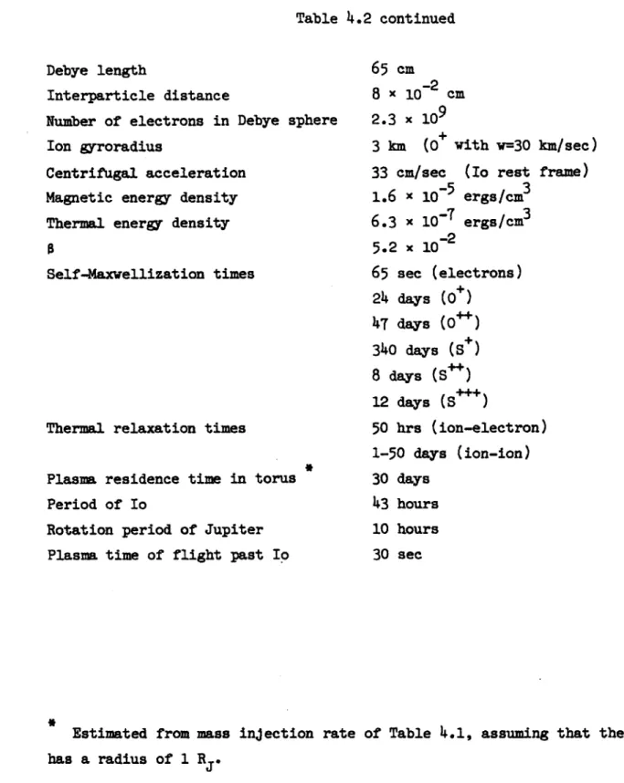
We then present analysis of data taken in the vicinity of the Jovian satellite Io. The interaction between Io and the Jovian

magnetosphere is a topic of considerable interest due to the fact that the decametric radio emmision from Jupiter appears to be modulated by the satellite. Unfortunately, the problem of determining the plasma parameters near Io is extremely difficult due to the low Mach number of the flow, the

large angle of the flow with respect to the cup look directions, and the

presence of several differeU ioPc specie . Under the assumption that the only ions present are 0 , 0 , S , and SO and that all of the ionic

species have the same thermal speed, we otain estimates of the plasma parameters by fitting seven spectra taken in the vicinity of Io. We

interpret our results in terms of a model of the interaction between Io and

the Jovian ionosphere due to Neubauer (1980). The results indicate qualitative agreement with the model that the flow is analogous to the potential flow of an incompressible fluid around an infinitely long cylinder.

Thesis Supervisor: Dr. Stanislaw Olbert

Acknowledgements

For helpful discussions and encouragement, I wish to thank Professors John Belcher and Ralph McNutt, and Drs. Alan Lazarus and Fran Bagenal.

For his assistance in the seemingly futile endeavor to tame the recalcitrant computer, I wish to thank Dr. George Gordon.

For their patience with my plottapes, I wish to thank Pamela Milligan and Mary Terkoski.

For her general helpfulness and cheerfulness, I wish to thank Anne

Bowes.

For his amazing ability to find money to support me term after term, I wish to thank Professor Herb Bridge.

There is more to life than physics, and I would not have been able to finish this thesis and retain Mr sanity without the help of many other people. In particular;

For his companionship as partner in frequent attempts to boldly sail where no windsurfer has sailed before, I wish to thank Dr. Paul Gazis.

For providing (too?) many hours of extremely enjoyable distractions, I wish to thank the staff of the Sailing Pavilion and the members of the MIT

Nautical Association.

For greatly enriching my life through the joy of music, I wish to

thank all of the people with whom I have played chamber music over the past

six years, in addition to the conductor, accompanist, and members of the MIT Choral Society.

For their frequent company and deep friendship, I wish to thank Peter

Shaw, Leslie Silverfine, Penelope Metzidakis, Roland Vanderspek, Donna

Hewitt, and Norman (Gil) Bristol, Jr..

For their love and moral support throughout my entire life, I wish to thank my parents.

And most important, for his many stimulating discussions of physics

and other topics, his infinite patience, his encouragement to help me through the all too frequent discouraging moments, his great generosity with his time, and numerous other things great and small, I wish to thank Professor Stanislaw Olbert.

Table of Contents Title Page p 1 Abstract p 2 Acknowledgements p 4 Table of Contents p

6

Chapter 2 Derivation of the Response Function of the

Voyager Plasma Science Experiment _{p 13}

Section 2.1 Location and Orientation of the Instrument p 14 Section 2.2 Structure and Operation of the Main Sensor Cups p 15

Section 2.3 Response Function of the Main Sensor p 17

Section 2.3a The Grid Transparency p 18

Section 2.3b The Sensitive Area p 20

Section 2.4 Structure and Operation of the Side Sensor p 24

Section 2.ha The Grid Transparency p 25

Section 2.4b The Sensitive Area p 26

Section 2.5 The "Cold Plasma" Approximation p 29

Section 2.6 The "Hot Plasma" Approximation for the Main Sensor p 32

Section 2.7 The "Hot Plasma" Approximation for the D-Cup p 37

Chapter 3 Experimental Test of the Response Function p 38

Section 3.1 The Cruise Maneuver p 39

Section 3.2 Analysis of Data Taken During the Cruise Maneuver p 41

Chapter 4 The Theory of the Interaction Between Io and the

Jovian Magnetosphere p 49

Section 4.1 Introduction _{p 50}

Section 4.2 The Equations Which Describe the Plasma at Io p 52 Section 4.3 The Io-Magnetosphere Interaction p 59 Chapter 5 _{Analysis of Plasma Data Taken in the Vicinity of}

Io by Voyager I p 73

Section 5.1 The Io Flyby p 74

Section 5.2 Analysis of the Data p 75

Section 5.3 The Flow Around the Alfven Wing p 82

Section 5.4 Summary _p 89 References p 92 Tables p 94 Figure Captions p 100 Figures _{p 113} Appendix A p 166 Appendix B p 178 Appendix C p 182 Appendix D p 186

Chapter I

On 20 August

1977,

a spacecraft named Voyager II was launched from the

Kennedy Space Center in Florida, bound for the outer solar system. Voyager I,

its sister ship, was launched two weeks later on September 5. Both spacecraft

were targeted for close encounters with Jupiter and Saturn. Voyager II will

also fly close to Uranus and Neptune.

One of the experiments carried by both of these spacecraft was a set of

four modulated grid Faraday cups called the Plasma Science Experiment (PLS).

The PLS experiment measures positive ions and electrons in the energy range of

10-5950 eV. It was designed and constructed at MIT, and includes several

novel features (Bridge et al). Three of its four cups are very shallow,

resulting in an extremely wide field of view. These same three cups are

arrayed about an axis of symmetry such that their fields of view overlap.

This region of overlap includes the direction of the solar wind flow

throughout most of the mission. By analyzing positive ion data taken by all

three of these cups simultaneously, it is possible to determine the direction

of the solar wind flow to better than one-half degree and its magnitude to

within a few km/sec.

The fourth cup is more conventional in design, and it looks in a

direction perpendicular to the symmetry axis of the main cluster.

During the

interplanetary, or cruise, phase of the

mission, this cup is used to measure

electrons.

In addition, during the inbound pass .of planetary encounters, this

cup looks in the direction of the corotating plasma, measuring both electrons

and positive ions.

The main sensor cups were designed in such a way that for a wide range of

sonic Mach numbers and flow directions, including all of the situations which

one expects to encounter during the cruise phases of the mission, almost all

of the particles which enter the aperture and are not stopped by the modulator voltage do reach the collector. During planetary encounters, however, the facts that the Mach number is frequently low and that the flow is highly oblique to the cups makes the "unity response" approximation not valid. In order to analyze data taken at these times, a knowledge of the full response function of the cups is required.

This thesis presents a derivation of the full response function based on a calculation of the trajectories of charged particles inside the cups. The

current measured by the sensors is given by the integral over velocity space of the product of the plasma distribution function and the cup response

function. A computer program which performs this integration numerically has already been written by V. Vasyliunas, one of the designers of the instrument. Unfortunately, his algorithm is very slow. Not only is it impossible to use

it to perform any iterative fitting procedure to determine the macroscopic plasma parameters, but it is even too slow to use at all for simulating the

high resolution (M-mode) energy-per-charge spectra. We have overcome this difficulty by approximating the analytic expression for the response function

by a functional form which permits the integrations over the components of

velocity perpendicular to the cup normal to be performed analytically for the case where the distribution function is a convected Maxwellian. This

derivation is the topic of Chapter 2.

In order to test the response function derived in Chapter 2, it is neccessary to have an extremely narrow test beam. Since such a beam is very

difficult to make in the laboratory and the quiet solar wind has just these properties, we have tested the response function by analyzing data taken by Voyager I during a cruise maneuver. During the cruise maneuver, the

cup response functions is the topic of Chapter 3.

On the outbound pass of its Jupiter encounter, Voyager I flew about 20,000 km above the south pole of the satellite Io. As the decametric radio burst from Jupiter are known to be correlated with the phase angle of Io, the interaction between Io and the magnetospheric plasma is a topic of

considerable interest. During the Io flyby, the sonic Mach number of the plasma was low (about 2) and the flow direction was perpendicular to the main sensor symmetry axis. This situation makes knowledge of the full response function neccessary for the analysis of the data taken during this period. This stretch of data was chosen for the first use of the full response function in analyzing data.

The satellite Io appears to have a high electrical conductivity. Drell, Foley and Ruderman (1965) have shown that any conductor which moves through a magnetized plasma will be a source of Alfven waves. If the velocity of the conductor with respect to the ambient medium does not change with time, there will be a standing wave pattern in the rest frame of the conductor consisting

of a pair of Alfven "wings" which extend away from the conductor in the direction of the Alfven characteristics. Neubauer (1980) has shown that the plasma flow around each of these wing is analogous to the potential flow of an incompressible fluid around an infinite cylinder.

The final two chapters of the thesis are concerned with Io's interaction with the Jovian magnetospheric plasma. Chapter 4 contains a discussion and critique of Neubauer's theory, while Chapter 5 consists of analysis of the

data taken by Voyager I during the Io flyby. We conclude that the data is consistent with the overall picture that the plasma flows around the Alfven wing as if the wing were a long, cylindrical obstacle.

Chapter 2

Derivation of the Response Function

of the

2.1 Location and Orientation of the Instrument

The Voyager Plasma Science Experiment consists of four modulated grid

Faraday cups. A sketch of the instrument is shown in Figure 2.1. Three of the cups, called the A-cup, B-cup, and C-cup, comprise the main sensor.

These three cups have the same pentagonal shape and are arrayed with their

cup normals 200 from an axis of symmetry. The fourth cup, called the side

sensor or D-cup, has a circular aperture. The normal to the D-cup aperture points in a direction 880 from the main sensor symmetry axis.

Figure 2.2 shows the location and orientation of the plasma instrument on the spacecraft. The instrument is mounted on the science boom, a metal support structure which extends away from the main body of the spacecraft. Also on the science boom are the cosmic ray, imaging, UV spectrometry, IR

spectrometry, photopolarimetry, and low energy charged particle experiments.

The system of coordinates called spacecraft coordinates is defined as follows: The spacecraft center of mass is taken as the origin. The

unit vector zsc points along the axis of the main antenna, with +sc

pointing into the antenna. The unit vector ysc lies in the plane

containing the zsc and the axis of symmetry of the science boom. It is

perpendicular to the 2sc and makes an acute angle with the science boom.

The unit vector

isc

The outward pointing symmetry axis of the PLS main sensor is parallel to -Z sc As this axis is also parallel to the axis of the main antenna, it is pointed at the earth during most of the mission. Since the angular separation between the earth and the sun as seen from the outer solar

system is small, the solar wind flow direction is substantially into the main sensor. The D-cup is oriented such that it looks into corotating flow during the inbound pass of a planetary flyby. The relative orientations of the cup apertures as viewed from along the main sensor symmetry axis is shown in Fig. 2.3.

During the interplanetary, or cruise, phase of the mission, the main sensor measures positive ions and the side sensor measures electrons. During planetary encounters, the D-cup is also used to measure positive

ions.

2.2 Structure and Operation of the Main Sensor Cups

A vertical cross section of a main sensor cup is shown in Figure 2.4,

and a top view is shown in Figure 2.5. The collector of the cup has the shape of home plate on a baseball field with the corners smoothed out. The aperture is similar in shape, differing in that it is smaller and its

parallel sides are shorter with respect to its other sides. The aperture

2

area (A ) is 102 cm . Around the edge of the collector is a rim of metal.

ap

The collector plane is considered to be the plane defined by the top of this rim. The distance (h) from the aperture to this plane is 4.1 cm.

The cup has nine parallel grids. Each grid consists of a woven mesh of two perpendicular sets of parallel wires. When measuring ions, the suppressor grid is held at -95V relative to the collector, and the same positive voltage square wave is impressed on all three modulator grids. The rest of the grids and the collector are grounded to the spacecraft. When a square wave voltage is impressed on the modulator grids, the

collector current is a square wave differing in phase by 1800, as shown in

Figure 2.6. The amplitude of this square wave is the information which is telemetered back to Earth. During operation, a sequence of such square

waves is used. The frequency of the wave is 400hz, and the limiting

voltages are changed every 0.240 secs. The voltages are changed such that

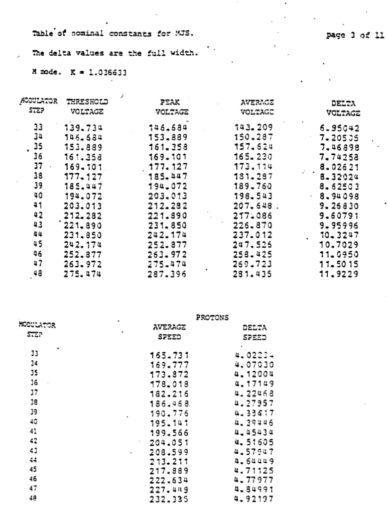
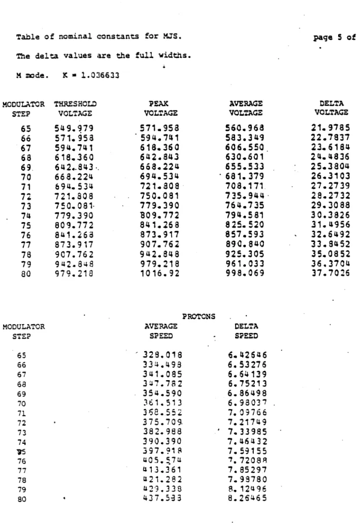
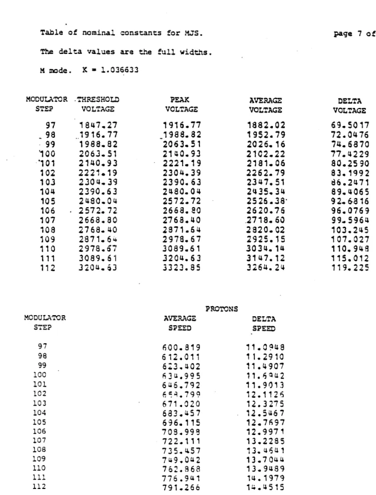
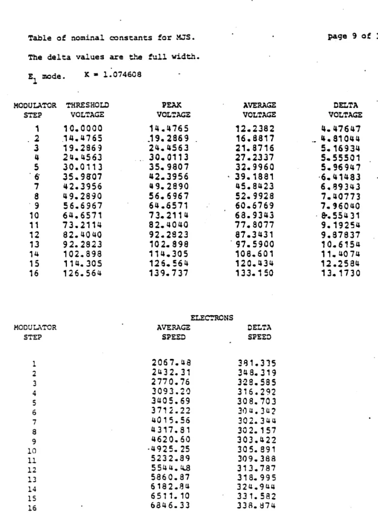
the higher voltage of any one square wave is the lower voltage of the next. In this way the voltage range of 10-5950 volts is divided into contiguous channels. In the low resolution (L-)mode there are 16 channels; in the high resolution (M-)mode there are 128 channels. Hereafter, we will label the channels with a subscript k. Appendix A includes a table which lists the threshold voltage #k, the voltage width Ak *k+1~ *k), and the average voltage 'k ((*k+l+

*

In order to define the threshold speeds vk we will use a coordinate

system called cup coordinates. We take as the origin the center of the long side of the aperture (point 0 in Figure 2.5). The unit vector 2 is

cup

perpendicular to the aperture plane and points into the cup, the unit vector xCUp is defined by the vector cross product of z s with Z cup and the unit vector gcup is defined to make a right-handed coordinate system.

Consider a parallel beam of positive monoenergetic ions incident on the cup. The only particles to reach the collector will be those with a z-component of velocity greater than vk given by

vk=(Zek/M)

*

where Z _{is the charge state of the ion, e is the elementary charge,}

_*

convient to define the average proton speed k and the channel width Avk as

rkk

Vk (vk+1+vk)/2 2.lb

Avk ~k+l~ k 2.1c

The values of 7k and Avk for each channel are included in Appendix A. In terms of the distribution function f(v) which describes the plasma environment of the spacecraft, the current in the k-th channel is given by Equations 2.2a and 2.2b.

* *

Ik k k+l 2.2a

I*=A Z e I ldv dv fdv v f(v)R(v,vk) 2.2b

kC 0W

y

where A0 is the aperture area times the transparency at normal incidence and R(V,vk) is the cup response function, to be derived hereinafter. The quantity

f(v) in the above equation is the distribution function of a single species;

if the plasma contains more than one species the current will be given by a sum of terms like Equation 2.2b, one for each type of ion.

The quantity Ik can be thought of as a function of vk. For the remainder of this thesis, the quantity I k(vk)/Ak will be referred to as the reduced

distribution function. This is because when the unity response approximation is valid, Ik/"k is in fact proportional to the object which generally goes by that name (see McNutt et al (1981)).

2.3 Response Function of the Main Sensor

Our problem is to determine the function R. A particle incident'on the

voltage, it collides with a grid, or its trajectory is such that it misses the collector and collides with the side of the cup. The first effect is taken

care of by the lower limit of the integration over vz; the latter two effects are included in R. R can therefore by written as a product of two terms and a normalization constant,

R=TA/A_{0 2.3}

where T is the transparency of the grids and A is the "sensitive" area of the collector. Note that R is normalized to unity at normal incidence. T and A are functions of velocity and channel number, while A0 is a constant. We will first consider the effect of collisions with the grids (transparency).

2.3a The Grid Transparency

The transparency of a single grid is defined as the probability of an incident particle traversing the plane of the grid without colliding with the wires. We model a grid as a planar structure consisting of two perpendicular sets of parallel cylindrical wires. In the main sensor, the sets of wires of all of the grids are parallel to the x- and y- axes in cup coordinates. The transparency of the grid will be the product of the transparencies of each set of wires considered separately.

Consider the wires which run in the x-direction. Since the transparency of these wires does not depend upon v , we only need to consider the

projection of the motion into the y-z plane. The probability of a particle

colliding with one of the wires is simply the ratio of the area of the wires to the area of the gaps between the wires projected into a plane perpendicular to the particle velocity vector (see Figure 2.T). Per unit length along the

wire, this ratio is

Probability of collision = d = c sec a 2.4

L cos a

where d is the wire diameter, L is the grid spacing, c(=1/42) is their ratio, and a is the angle between the particle velocity and the grid normal. The probability of a particle not colliding with the grid, is

Probability of no collision = 1- (c sec a) 2.5 If v* is the velocity of the particle as it crosses the grid plane, we see that the transparency of one grid is

v* 2₁ 2V21/

T=[l-,(1+ _V*V2/l[-+( 27/) 2.6

z z

Under the assumption that the potential inside the cup depends only on z,, v* depends solely upon the velocity of the particle before it enters the cup and the voltage on the grid. The validity of this approximation will be discussed in the next section. An expression relating v* with v is now found from

energy conservation to be V* _x = VY 2. Ta v* = v 2.Tb y y V* = (v2 - 2e /Am )1/2 _2.Tc z z p

The transparency of all of the grids is the product of the transparencies of the individual grids. It is given by

2 2 Vi v l' T=H1-c(l+ )1/2I (1-c(l+

)1/2

where is the voltage on the i-th grid

Each cup has three modulator grids, one suppressor grid, and five

by v2,2 2 T=[1-c(l+ -) 1/2]5[1-ce(,+ vx 2 1/213[1-c(,+ 2 y1/2 x

2

vs2

z

z

v )125lv

_y

)_/25

2

vz('

2

Tz (:.i

The subscript s refers to the suppressor grid; vs is defined in a manner analogous to the definition of vk in Equation 2.1

v =(2Z*e#₈/Amp )1/2 2.10

where

*s

Note that for normal incidence T=T 0=(-c)18=0.65 and AO=66 cm2.

2.3b The Sensitive Area

The second factor in Equation 2.3 is the "sensitive area". This is defined to be the overlap of the area of the collector with the area of the image of the aperture in the plane of the collector.

Consider a beam of particles incident at an angle a to the cup normal. In the collector plane, the beam will have the shape of the aperture, but its position will be displaced because of the components of the particle velocity transverse to the cup normal direction, as shown in Figure 2.8. First we will

compute the amount of the shift., and then we will discuss the functional dependence of the sensitive area on the shift vector.

We define a two dimensional vector , also shown in Figure 2.8, to be the

aperture into the plane of the collector. Figure 2.9 shows the projection into the x-z plane of a possible trajectory of a positive ion as it moves from the aperture to the collector of one of the main sensor cups. If the

particles were not deflected by the electrostatic fields inside the cup, the shift would be given by

xv

S = -- h 2.11a

Z

S = - h 2.llb

y vz

The effect of the fields is to bend the beam, thereby changing the amount of the shift. To compute the amount of the shift, we will solve the equations of motion for a charged particle moving in the electric field of one of the cups.

We will assume that the potential between the grids depends only upon z. This neglects the fine structure of the fields close to grids as well as the

fringing fields near the edges of the grids.

The fine structure of the fields in the vicinity of the wires decays in a

distance comparable to the mesh size of the grid. Since this distance is much

less than the spacing between grids, the ripple in the fields near the wires can safely be ignored.

The fringing fields are important only in a region around the edge of the grids which has a width comparable to the grid spacing. Because of the cup goemetry, any particle whose trajectory includes the region where the fringing

fields are important will miss the collector. As.this will occur whether or not the fringing fields are used in computing the trajectory, these fields can be ignored.

The potential is therefore well approximated by a linear function of distance between any two neighboring grids. Figure 2.10a shows the potential

as a function of z for a typical channel. Using energy conservation and the

fact that the fields are entirely in the z-direction the equation of motion is

easily solved. The equations of motion of the particle are

V* dx = v 2.12a

x

dt

x

dz

.762

k

(z)= 3.089-z

#

2.700<z<3.089

2.13f

Equations 2.12a and 2.12b can be solved by inspection. For a particle which crosses the aperture plane at the origin of the cup coordinate system, the

result is

x=v t 2.14a

Y-v t 2.14b

y

The components of the shift vector are simply the values of x and y

evaluated for t equal to the transit time of the particle from the aperture to

the collector plane. This can be evaluated with the aid of Equation 2.12c, which can be rewritten as

t _h

dz

fdt = I _(

2

z Am

Inserting the expressions for $(z) from Equations 2.13a-2.13g and performing the integrations we find

t=t +tb +t +t +t +t f+t 2.16 2 IV -)1/2 1-2 V t (.762 z 2.17a a v z (v 2 2 z k tb=(. v X )2.1Tb z v

(1-

-)

td

[(1+

)1/2

(2 )(.414)

Using Equations 2.14a, 2.14b, 2.16, and 2.17a-2.17g the shift vector can be written as

S = S(

)h

2.18a

z

S

y=

S(

I

)h

2.18b

with S, the shift function, defined by :2 2 (1-( k)1/2] _[

₎₍₊

2

1(+2

+.392(

(v /v

)

1-(vv

/V)

(v /v )

We shall now very briefly consider the sensitive area as a function of the shift vector, which we will denote by A(S). Because of the shapes of the aperture and the collector, this functional dependence is complicated. As there are 16 separate regions where the dependence is different (see Figure 2.11), an analytic representation is cumbersome. A(S S y) is given in tabular

form in Table 1. A plot of the sensitive area as a function of S y with S as

y x a parameter, is shown in Figure 2.15.

2.4 Structure and Operation of the Side Sensor

The geometry of the D-cup is quite different from that of the main sensor cups. Figure 2.12 shows its cross section. Its aperture and collector are circular, and it has a metal annulus called the guard ring which is located 1.4 cm above the collector. The outer edge of the guard ring is connected to the side of the cup, while its inner diameter is smaller than the diameter of the aperture. The radii of the aperture, guard ring, and collector are 5.64

cm, 5.13 cm, and 6.35 cm, respectively. The distance from the collector to

the guard ring is 1.413 cm, and from the collector to the aperture is 6.000 cm. It has eight grids, two of which are suppressor grids and only one of which is the modulator grid for the positive ion mode. The potential as a function of position for a typical channel is shown in Figure 2.10b.

In addition to measuring positive ions, the D-cup-is also used to measure

electrons. A different modulator grid is used for the electron mode. The

potential as a function of position for a typical channel in the electron mode

is shown in Figure 2.10c. The voltage thresholds for the two electron modes

are included in appendix A.

2.4a The Grid Transparency

We will first consider the transparency function for the D-cup. The only

complication not found in the main sensor cups is caused by the fact that the

wires meshes in the different grids are not parallel to each other, but are

rotated relative to each other by a specific angle. Also, the Voyager I and

Voyager II instruments are different from each other. The mesh orientations

for both spacecraft are given in Table 2.2.

We define cup coordinates for the D-cup a fashion analagous to that used

for main sensor cups; the z

cup-axis is parallel to the cup normal and points

into the cupq CUp =sc X

,cup

xcup.

coordinate system is defined to be the center of the aperture. The

transparency of any grid is still given by Equation 2.6 provided vx and vy are

interpreted as the components of velocity along the directions of the grid

wires. The grid orientation as given in Table 2.2 can then be used to rotate

from cup coordinates to "grid" coordinates. The resulting expression for the

transparency of the D-cup is

6 2 V2

T= _1-c(l+ - cos2( -a )) 1 [1-c(l+ sin (t-a))1 j x

z z

-2 2 2 2

v cos (t-a

)

Ii-c

(i+

2

)1/2Il-c

(1+

2

)J

2 2 v2

v (1- ) v (1- M)

2 2 2. 2

z

z

2 Cos 2 (-a / _{sin (-as}

1l- tl F S )1/2J Il-( 2t 2__V / 2 V ( - )2 [ -c(s v (1- 8) v (1- S) z v2 v2 z z

where the a's are the angles from Table 2.2 which describe the grid orientation, and t and Vt are defined by

V =(V2+v2) 1/2 2.21a

t x y

t=arctan(vy/v x) 2.21b

At normal incidence, T=TO=(1-c) 16=0.68 and AO=56.2 cm2.

2.4b The Sensitive Area

We now proceed to the sensitive area calculation. Because of the guard ring, the sensitive area is the mutual overlap of three circles of different sizes, the centers of which lie on the same line. There are now two

independent shift vectors, one for the collector-guard ring shift and one for the collector-aperture shift. Because of the circular symmetry, the sensitive area does not depend upon the direction of the shift vector, only its

magnitude. We therefore assume, without loss of generality, that the velocity vector of the incident beam lies in the x-z plane. By assumption, the

magnitude of the (x-directed) shifts between the aperture and collector and between the guard and collector, respectively. It is also convenient to

define Sag as the relative shift between the aperture and the guard ring,

S

=s -s.

ag ac ge

We will now derive an expression for the overlap area of two circles with radii Rs and RL (RL>Rs) whose centers are separated by a distance S, as shown in Figures 2.13a, 2.13b and 2.13c. Let the coordinates of the centers of the circles be (0,0) and (s,0). The equations of the two circles are

X2+y2=2 _2.22a

(x-s)2 +y 2=R2 2.22b

s

An important parameter, which we shall call X, is the x-coordinate of the points where the two circles intersect (see Figure 2.13b). X can be

determined as a function of s, RL, and Rs by subtracting Equation 2.22b from 2.22a and solving for x. The result is

2 -2+2

X= 2s _2.23

Note that X as defined by Equation 2.23 is real and well defined even when the circles do not intersect. In this case X>RL and the corresponding value of y which simultaneously satisfies Equations 2.22a and 2.22b is imaginary. We shall find it convienient to define X by Equation 2.23 even when the

geometrical interpretation of it no longer holds.

Now consider the following three cases, as shown in Figures 2.13a, 2.13b,

and 2.13c.

Case I _szRL-Rs

In this case the overlap area is obviously just the area of the smaller circle.

A=wR 2.24a

Case II _{R1-Rs<s<RL+Rs}

The overlap area is given by the following sum of two integrals.

XR

A= X [(x-s)2_-R2 _1/2_{dx + jL I2-R I/dx}

2.25

s-R5 X

This integral is elementary, yielding

A=R2 [2 + arcsin Q (1-Q1)1 /21+R2

[1 -

Q

)

1 2sR

In this case the overlap area is zero.

A=0 2.24c

We shall denote by X and X the x-coordinates of the points of

ac g

intersection of the image of the aperture in the plane of the collector and

the collector and of the image of the guard in the plane of the collector and

the collector, respectively (see Figure 2.14). These can be evaluated with

Equation 2.23 by substituting the radius of the collector for RL, the radius

of the aperture(guard ring) for Rs, and S ac(S g) for s.

To determine the overlap area of the three circles, one must consider the

following two cases; Case A: X >X

gc ac

This is the most frequently encoutered case, and it covers several apparently different situations. These are all shown in Figures 2.14a-2.14c. For all of these cases the sensitive area is given by

A=A +A g-A 2.2Ta

of the guard ring and the collector, respectively, as given by Equations 2.24a-2.24c, and A is the area of the guard ring.

Case B: X =X gc ac

For this case, shown in Figure 2.14d, the sensitive area is the overlap area of the aperture and the collector.

A = Aac 2.2Tb

This completes the derivation of the cup response function.

2.5 The "Cold Plasma" Approximation

The problem of data reduction now formally reduces to inverting a set of integral equations like Equations 2.2 to solve for the distribution function. Unfortunately, this task is very difficult, and a unique solution may not exist. The approach which we have adopted involves paramaterizing the

distribution function and then searching parameter space for the "best fit" to the data.

From statistical mechanics we know that the distribution function which describes a gas in thermodynamic equilibrium is the Maxwell-Boltzmann

distribution

-- N 0 2 2

f(v) 3/ 3 exp-(v-V)

w

ir w

where N is the particle number density, V is the bulk flow velocity, and w is the thermal speed. Although neither the solar wind nor the Jovian

magnetospheric plasma is in local thermodynamic equilibrium, there is some empirical justification for using this form for the distribution function. It can be shown that distributions with more than one peak are unstable, and in

the vicinity of the peak one expects the distribution function to be bell

shaped. We shall therefore assume that the distribution functions can be approximated by expressions like Equation 2.28.

We now must evaluate the integrals in Equation 2.2b. This cannot be done analytically without further approximations. For the case of a "cold" plasma, i.e. when IVI/w>>l, we can approximate the dependence of f('V) on the

components of velocity transverse to the cup normal by a product of two delta functions

N

2

f(V)= 6(v -V ) 6(vy-v ) exp{-(vz-z) 2v 2} 2.29

This permits the integrations over v and vy to be performed trivially. The

result is

N

I = exp(-(v z 2_/ 2_{) R(V XV ,}

9 vz) dvz 2.30

vk

For the D-cup, Equation 2.2b can be evaluated numerically using Equations 2.20, 2.21 and 2.23-2.27. For the main sensor Table 2.1 must be-used in

addition to Equation 2.9. The use of the lookup table can be eliminated by fitting the area overlap with an easily evaluated function. This approach will be particularly important for the "hot plasma" approximation described

hereinafter.

The family of curves representing the sensitive area is shown in Figure

These functions will be fit by the "trapezoidal approximation"

A=A (S /h)A (S /h,S /h)=A, (S /h)C(S /h)A (S /hSy//h)

A= x r (s /h) -X'<S /h<X x X'-X x r x r

r r

1

r

(S/)

-X

Otherwise

2.32a

2.32b

2.32c

2.33d

(S /h)-Y (S )

0

X

X'

=4. 94

r

y

Y'=-3.62

_d

.762 cos{1.018(S /h)+.247}

2.3

e

Y'=2.50-0.125 [(S/h)-1.2

2.34f

x

x

x

All of the quantities defined by Equations 2.34a-2.34f are dimensionless.

Yu

and Yu' are plotted in Figure 2.16. Fiqure 2.17 shows the

trapezoidal

approximation for A plotted versus S

y/h with

S

/h as a parameter, while Figure

2.18 shows A plotted versus

S

/h for S equal to

0.

Figure 2.19 shows a 3D

plot of A(S). The values of X

,

X1'

9d'

_r

_VYA

_r

A'

,

and Y' were chosen so as to

A

x

A

y

y

2.33e

2.33g

2.33h

2.34a

2.34b

2.34c

2.34d

match the volume of the solid of Fig. 2.19 as closely as possible with the

volume of the solid representing the true area overlap. Figure 2.20 shows a

3D plot of R(S /h,S /h)

for which the "trapezoidal" approximation was used to

eveluate the sensitive area and Eq. 2.9 was used to compute the transparency.

Appendices B and C contains listings of Fortran programs which compute the

integrals in Equation 2.2b for the main sensor cups using the "trapezoidal"

approximation and for the D-cup, respectively.

The "cold plasma" approximation was used to test our theoretical response

function

by analyzing data taken during a cruise maneuver, as described in the

next chapter.

2.6 The "Hot Plasma" Approximation for the Main Sensor

When the thermal speed of the plasma is comparable to the magnitude of

the bulk

streaming velocity Equation

2.30 is no

longer valid. This is the

case during Voyager I's

pass near the Io flux tube.

To perform the integral

of Equation 2.2b in this case we have fit the previously derived expression

for the transparency, Equation 2.9, by an expression with a functional form

which permits the integrals over v and v to be performed analytically. The

x

y

expression we have used is a sum of two Gaussians

2

2

v

T=-TO

_0.i~

.E

ZC

_cjicex

excp(-a.(

_i

(

2.35

3

2

J

v2

i=1 j=

vz

2 2

2 2

where c , cj, ai, and aj are functions of vZ /k and of v

2/v, and T

is the

transparency at normal incidence. The values of the c's and a's were

determined from Equation 2.9 by the following procedure: We reduced the

integral over v and y of Eq. 2.2b give the correct answer for an infinitely

hot plasma, and then did a nonlinear least-squares fit to determine the best

values for the a's and c's.

Using a Maxwell-Boltzmann distribution (Equation 2.28) for f( o), the "trapezoidal approximation" (Equations 2.31-2.34) for A, and Equation 2.35 for T, Equation 2.2b becomes T z*eN * (v

-V

v2

(v -V )

(v-V )

IA Z c c exp{-a-2i -a-- - 2 }dv dvy

-- -- ij v v w

z

z

It wiU be convient to perform the following change of variables

X = Svx/vz = Sx/h 2.3Ta

Y = Svy/v =S Sy/h 2.3Tb

After some algebra Equation 2.36 becomes

N ez*T R a

v

-V

3

0 _{k- 1323v} fjdXdY z2

_{2 exp(-}

)0

_{ij jix jy}

₃

2 2

2aiw

a w

C.

v2+a w yv+a w G =exp{-a (X-a )2} 2.39b G₃y=exp{-a (Y-a )2 2.39c a.w2 +v2 2 z 2.39d Sv x w X= 2.39e V2+a w2 Sz I Z = -- _2.39f V +a w2

zJ

2.39g

We are now ready to carry out the necessary integrations. We will

perform the integral over Y first. Regrouping terms in Equation 2.36 we find N 0z*eT0 A0

I*= /

.E

s

2

2

v z 2 2( a w 2 w2

D ij=c C expf-[(- - z +11 2 2 )+1y2 2)]}

2.40b

w v +a w v +a w

The Y-integration can be expressed in terms of elementary functions and the Gaussian error function. The result is

- /, T(Z

*(Z')-

H

f(X)=

=

}

2.41a

-a 2/a Z'-Z

Z

J

u

d

*(Z)=Z erf(Z) +(l//w)exp(-Z

)

2.41b

Zd=/ ( d MX) aj) 2.41c

ZA=7/0

(Yu(X)--)

2.41d

Zu=a (u(X)--V ) 2.41e

Z'=/Q (Y'(X)-a )2.41f

u

u

J

Equation 2.36 now becomes

Noz*eTOA

2

2

w.

2

x

2z

{fdv[-

zD LdX AX(X)G.X(X)H

(X)JI)24

k W3/2 3 i~

jz _aZS

ii

Ai

Since the integral over X is now very complicated, it cannot be done without

further approximations. If H

(X)

is a slowly varying function of its

argument, we can use the saddle point method to write the integral over X as

fdX AX(X)GiX(X)Hj (X) H (R )E((X) dX AX(X)GiX(X) 2.43a

I XI AX(X)GiX(X)dX

2.43b

1 a

JAX(X)GiX (X)dX

-M

Again, all the integrals can be expressed in terms of elementary functions and the Gaussian error function. The results are

CO /

(Z

X

=-X'=-4.94

2.44g

1r

)+(Z')-

)+

_2a

T(Z)=(a /a Z-(1/2))/lw erf(Z)+a / a exp(- 2) 2.44 We now sumarize the results of this section by rewriting Eq. 2.2 in terms

of the functions defined by Eqs. 2.19 and 2.39-2.44 as

z*eTOAONO 2 2 a v D

I*= _4/ww3 I X

ffdv

The integral over vz in Eq. 2.45 must be performed numerically. To devise an efficient scheme for calculating Ik for many adjacent channels, we

shall rewrite Eqs. 2.2a and 2.2b as

vk+l O

Ik = I dvz Q z' k) + I dvz (Q(vz vk)-Q(vz'vk+l) 2.46

vk+l

where Q denotes the integrand of Eq. 2.45. The contribution from the second integral on the right side of Eq. 2.46 is called the feedthrough current. The dependence of Q upon vk is implicit in its dependence on the a's and c's. Since the a's and c's are slowly varying functions of vk for vz<v k, we can expand the second integrand in Eq. 2.46 in a Taylor series in the a's and c's.

Q(V

(aQ/ac₂)(c2(V zvk)-c2(vz vk+)+(aQ/aal)(al(vzgvk)-al(vzvk+l)+ 2.47

(BQ/3a2)(a 2(vz' k-a2(vz' _k+1)

This enables us to use compute one value of Q(vz) and use it in the numerical integration of several channels, greatly reducing the amount of computer time required to simulate an M-mode. Appendix D contains the listing of a Fortran program which utilizes this technique to simulate an M-mode spectrum. We

expect that this program can simulate the response of the main sensor cups to

2.7 The "Hot Plasma" Approximation for the D-Cup

Except for a small effect due to the alignment of the grids, the D-cup response is azimuthally symmetric about its z-axis. Therefore, the response can only depend upon v +v2 and cannot depend upon v and vy individually. We have fit the the full response function by a function of the form

3 v2 2

R(v,vk'v s . c exp{-ai 2 1} 2.48

i=l

v

z

where once again the a 's and c 's are functions of v2 /0 and *s. Using a

Maxwellian for the distribution function and Equation 2.48 for R in Equation

2.2b we obtain

3 AoToNoz*e (v z

-V

Ik 1 1i 3/2

W3

z

z

w2

2

2

2

22.9

Ce (v -V) ajv x o (vy-Vy) a v

lexp{- x 2 - v1 x exp{- w 2 - ydv

- w 2v

_z

_z

The integration over the transverse components of the velocity are easily done, yielding

3 AoToNoz*e vzdvz v -V a (V2+V2)

=Z C. 0 vv exp-( (e ) - } 2.50

k

k

w2/v

As in the case of the main sensor cups, the integration over vz must be done numerically.

This completes the discussion of the response function of the Voyager PLS

Chapter 3

3.1 The Cruise Maneuver

Before the formulas derived in the preceding chapter can be used with

confidence to analyze data, they should be tested. Attempts to measure the

response of the cups as a function of angle were made prior to launch.

This was done by placing the instrument in an evacuated chamber in the path

of a beam of charged particles. Data were then taken with the instrument

in different orintations.

Unfortunately, it was not possible to test the cup response function

to the desired accuracy. Tests were performed with both a proton beam and

an electron beam. Since the quantity which is measured is an integral over

velocity space of the product of the response function and the distribution

function (Eqs. 2.2a,b), it is desirable to have a beam with a small thermal

velocity dispersion. The proton beam had too great a velocity dispersion

for the desired measurement. The electron beam, although sufficiently

narrow, caused the emission of a large number of secondary electrons which

contaminated the data. In particular, the response at large angles of

incidence was different from what was expected.

The quiet solar wind, on the other hand, has ideal properties for use

as a test beam. At 1 AU, the magnitude of its bulk streaming velocity is

typically eight times its thermal speed, and this ratio increases with

distance from the sun. In order to test the response function, however,

the direction of the test beam must be varied. Since the direction of the

solar wind is steady to within a few degrees, this requirement can only be met by rotating the spacecraft.

On 14

September 1978, Voyager I, then 4.1 AU from the sun, executed a

series of rotations called a cruise maneuver. Data from this particular

maneuver were selected for analysis because during it the solar wind was

quiet and the Mach number of the flow was high (-.20). The maneuver consisted of ten rotations about the spacecraft z-axis(rolls), ten rotations about the spacecraft y-axis(yaws), and ten more rolls. Each rotation took about 33 minutes. Since the symmetry axis of the main sensor

is aligned with the spacecraft z-axis, only the yaws are useful for the purpose of determining the cup response because the angle of the solar wind to the cup normals does not change appreciably during the rolls.

During the cruise maneuver the PLS experiment was taking one M-mode measurement every 96 seconds. Due to telemetry rate constraints, the data from all 128 channels of each spectrum was not sent back to Earth. On alternate spectra, the data from channels 1-72 and 57-128 were transmitted. During the maneuver the solar wind speed was about 380 km/sec, so the peaks in the spectra were never in a channel higher than about 68. Thus, only the spectra containing channels 1-72 could be used for analysis when the

beam was oblique to one or more of the cups.

Due to a coincidence, the period between PLS M-mode spectra and the rotation period of the spacecraft during the maneuver were almost

commensurate, resulting in the spacecraft having almost the same orientation at the times of corresponding spectra taken in different rotations. Since an odd number (21) of M-mode spectra were taken during

each rotation, an upper-half spectrum was taken with the spacecraft in the

same orientation as a lower-half spectrum from the previous rotation. Weo

therefore did not lose any angular coverage due to the fact that only 72 of the 128 channels were available from each spectum.

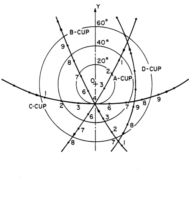
The angular coverage of the cruise maneuver is shown in Figure 3.0, which is a polar plot of a unit vector which points radially away from the

sun. This vector, the nominal solar wind direction, is plotted in cup

coordinates at the times of the start of the M-modes for each of the four

-.

cups. The polar angle 0 and the azimuth angle $ of a vector V are defined

by Equations 3.la and 3.lb

O=cos- (v //e(V2+V2+V2)) 3.1a

z x y z

*=tan (V /V ) 3.lb

y x

where V,, Vy, and Vz are the cartesian components of V. The numbered points in Fig. 3.1 correspond to the spectra which were analyzed as described hereinafter.

3.2 Analysis of Data Taken During the Cruise Maneuver

To test the response function we adopted the following strategy. We analyzed data from all of the orientations for which there were signals in

at least three of the four cups. We then did a simultaneous fit to these data using the "cold" plasma approximation described in Section 2.5. The derived macroscopic plasma parameters were then compared with each other. We also fit an additional spectrum taken when the plasma flow direction was

almost aligned with the main sensor symmetry axis. In this case we expect the "unity" response approximation to be valid. Since we have confidence

in the parameters we derive at these times we can estimate how much the solar wind is changing between the times of the other measurements and see

if the parameters derived from the other measurements stay reasonably

steady. If they are, this fact and the goodness of the fits indicates how well we understand the response function. In addition, comparison of the parameters derived from the fits of the solar wind using the "unity"

fits to these same spectra using the "cold beam" approximation indicate the

systematic error, if any, which the former approximation introduces. Nine spectra taken during the cruise maneuver were analyzed. The numerical integrations in Equation 2.30 were done using Simpson's rule. For a term with velocity threshold vk, we chose a step size of

Avk/10. Since the integrand is formally undefined at vz k, the proper

limiting value of zero was used.

The spectra consist of a background and one or two peaks. The main

peak, due to protons, was fitted. In each cup, about twelve channels around the peak were included. The fits have five parameters; the three

components of bulk velocity in spacecraft coordinates, the density, and the thermal speed. The velocity was then rotated into cup coordinates and the

currents were computed.

The criterion used to define the "best" fit was the minimization of X , defined by

X 2=Z(D.-A) 2/(.o4D )2 3.2

where each of the D i's is the measured current divided by the channel

voltage width and the A. 's are the simulated reduced distribution

functions. The solution to the extremum problem was found using a gradient

search algorithm similar to that described in Bevington (1969). The

derivatives with respect to the velocity components and thermal speed were computed numerically, while the derivative with respect to the density was computed analytically.

The results of the analysis of the cruise maneuver are shown in Table 3.1 and Figures 3.2-3.10. Figure 3.2 corresponds to point 1 in Fig. 3.1,

distribution function versus velocity for the nine spectra used. The data

are represented by the "staircase" while the fit is represented by the smooth curve. Table 3.1 lists the time, the wind velocity in RTN

coordinates, the density, and the thermal speed derived from the fits for each of the spectra. (RTN coordinates are a sun centered orthogonal

system. r points radially away from the sun;

£

The variation in these parameters is about what one expects to find in

a quiet solar wind, and the fits are quite good. The fits correctly

reproduce the relative heights, positions, and shapes of the spectra in the oblique cups.

The question of choosing the proper criterion for determining the

"best fit" deserves more discussion. If one chooses to minimize the square

of the difference between the data and the fitting function, there remains the problem of choosing the proper statistical weights. This choice must be made by analyzing the sources of error in the measurement. In our case, there are two main sources of error; electrical noise and digitization

error. Since the logarithm of the currents is digitized, this error is a

fixed percentage of the signal. This accounts for the weight factor of 1/Q.04D2 in Eq. 3.2. The electrical noise is a more difficult problem. We

expect thermal fluctuations in the amplifiers to be seen as fluctuations in

the current. The rms power in these current fluctuations should be about

the same in all of the channels. Since the reduced distribution function is the current divided by the channel width and the channel width increases with increasing channel number, this component of the noise should be most

An example of spectra which we expect to be entirely noise are the

D-cup spectrum in Fig. 3.4 and the lower channels in the main sensor cups in the same figure. The predominately smooth trace is due to the signal

being less than the minimum that can be digitized with our coding scheme; the fluctuations are noise. The predominant smoothness of the curve, especially the lower channels in the B-cup, indicate that the true thermal noise is below the threshold of the detector. We conclude that the noise which we see has another origin. Other sources of noise, such as cosmic

rays or interference with other instruments on the spacecraft, are more difficult to estimate. I have accounted for them in nqr selection of which channels to include in the fits. Unless specifically mentioned, all of the graphs of the results of fits to spectra include all of the data in a

particular spectrum and the simulations for all of the channels used in determining the best fit, and no others.

The question of estimating the uncertainty in the macroscopic plasma parameters derived from the previously described fitting procedure deserves

discussion. The formal uncertainty in the fit parameters is contained in the so-called error matrix. The properties of this matrix are described in Bevington (1969). The uncertainties which I quote throughout the remainder

of this chapter are defined by 2 2

"i =ii X /nf 3.3

where a. is the formal uncertainty in the determination of the i-th parameter, c is the error matrix, and nf is the number of degrees of

freedom (number of data points/number of parameters). In the case of linear parameters and Gaussian statistics, a is simply the standard

deviation one would expect to find in the value of the i-th parameter if the same experiment were done many times.

If the uncertainty in the individual data points can be accurately

2

2

estimated, a2 is simply equal to e. Unfortunately, the values of x we obtained in the fits of the cruise maneuver were sufficiently large to convince us that we had underestimated the uncertainty in the measurement.

The factors which multiply c in Eq. 3.3 are an attempt to compensate for

this underestimate.

In addition to random errors estimated by a, there is always the possibility of some systematic error. There are many possible causes for systematic errors. They can be related to the detector, such as

uncertainty in the values of the threshold voltages, or they can be

related to the plasma itself, such as the presence of suprathermal tails to

the distribution functions or thermal anisotropy. In general, systematic

errors are more difficult to estimate than random errors.

3.3 Discussion and Conclusions

An examination of Table 3.1 shows that the formal errors in the

density and thermal speed are about 3%. In addition, the magnitude of the bulk flow velocity is determined with a precision of less than one percent, and the direction is determined to within 10 arcseconds. We expect that the systematic errors in the determination of these quantities is

considerably larger.

The quality of the fits, even at large angles of incidence, gives us

great confidence in the accuracy of the response function. For example, compare Figures 3.1, 3.la, 3.lb, and 3.5. (The following numbering scheme is used; the spectrum in Figure 3.n was taken when the orientation of the spacecraft was such that the nominal solar wind direction corresponded to