Measurement of the differential cross section d\sigma/dt in elastic $p\bar{p}$ scattering at sqrt(s)=1.96 TeV

arXiv:1206.0687v1 [hep-ex] 4 Jun 2012

Measurement of the differential cross section dσ

_√

/dt in elastic pp scattering at

s = 1.96 TeV

V.M. Abazov,33 _{B. Abbott,}71 _{B.S. Acharya,}27_{M. Adams,}47 _{T. Adams,}45 _{G.D. Alexeev,}33 _{G. Alkhazov,}37 A. Altona_,59_{G. Alverson,}58_{G.A. Alves,}1_{M. Aoki,}46 _{A. Askew,}45 _{S. Atkins,}56 _{K. Augsten,}8_{C. Avila,}6 _{F. Badaud,}11

L. Bagby,46 _{B. Baldin,}46_{D.V. Bandurin,}45_{S. Banerjee,}27_{E. Barberis,}58 _{P. Baringer,}54_{J. Barreto,}2_{J.F. Bartlett,}46 U. Bassler,16_{V. Bazterra,}47 _{A. Bean,}54_{M. Begalli,}2 _{L. Bellantoni,}46 _{S.B. Beri,}25 _{G. Bernardi,}15 _{R. Bernhard,}20

I. Bertram,40 _{M. Besan¸con,}16 _{R. Beuselinck,}41 _{V.A. Bezzubov,}36_{P.C. Bhat,}46 _{S. Bhatia,}61 _{V. Bhatnagar,}25 G. Blazey,48 _{S. Blessing,}45_{K. Bloom,}62 _{A. Boehnlein,}46 _{D. Boline,}68 _{E.E. Boos,}35 _{G. Borissov,}40 _{T. Bose,}57 A. Brandt,74 _{O. Brandt,}21 _{R. Brock,}60_{G. Brooijmans,}66_{A. Bross,}46 _{D. Brown,}15 _{J. Brown,}15 _{X.B. Bu,}46 M. Buehler,46 _{V. Buescher,}22 _{V. Bunichev,}35_{S. Burdin}b_,40_{C.P. Buszello,}39_{E. Camacho-P´erez,}30_{W. Carvalho,}2

B.C.K. Casey,46_{H. Castilla-Valdez,}30 _{S. Caughron,}60_{S. Chakrabarti,}68 _{D. Chakraborty,}48 _{K.M. Chan,}52 A. Chandra,76_{E. Chapon,}16_{G. Chen,}54 _{S. Chevalier-Th´ery,}16 _{D.K. Cho,}73_{S.W. Cho,}29 _{S. Choi,}29 _{B. Choudhary,}26

S. Cihangir,46 _{D. Claes,}62 _{J. Clutter,}54 _{M. Cooke,}46 _{W.E. Cooper,}46 _{M. Corcoran,}76 _{F. Couderc,}16 M.-C. Cousinou,13 _{A. Croc,}16 _{D. Cutts,}73 _{A. Das,}43 _{G. Davies,}41 _{S.J. de Jong,}31, 32 _{E. De La Cruz-Burelo,}30

C. De Oliveira Martins,2 _{F. D´eliot,}16 _{R. Demina,}67 _{D. Denisov,}46 _{S.P. Denisov,}36 _{S. Desai,}46 _{C. Deterre,}16 K. DeVaughan,62 _{H.T. Diehl,}46 _{M. Diesburg,}46 _{P.F. Ding,}42 _{A. Dominguez,}62 _{A. Dubey,}26 _{L.V. Dudko,}35 D. Duggan,63 _{A. Duperrin,}13 _{S. Dutt,}25 _{A. Dyshkant,}48 _{M. Eads,}62 _{D. Edmunds,}60 _{J. Ellison,}44 _{V.D. Elvira,}46 Y. Enari,15_{H. Evans,}50 _{A. Evdokimov,}69_{V.N. Evdokimov,}36 _{G. Facini,}58 _{L. Feng,}48_{T. Ferbel,}67 _{F. Fiedler,}22

F. Filthaut,31, 32 _{W. Fisher,}60 _{H.E. Fisk,}46 _{M. Fortner,}48 _{H. Fox,}40 _{S. Fuess,}46 _{A. Garcia-Bellido,}67 J.A. Garc´ıa-Gonz´alez,30_{G.A. Garc´ıa-Guerra}c_,30 _{V. Gavrilov,}34_{P. Gay,}11 _{W. Geng,}13, 60 _{D. Gerbaudo,}64 C.E. Gerber,47 _{Y. Gershtein,}63_{G. Ginther,}46, 67 _{G. Golovanov,}33_{A. Goussiou,}78_{P.D. Grannis,}68 _{S. Greder,}17

H. Greenlee,46 _{E.M. Gregores,}3 _{G. Grenier,}18_{Ph. Gris,}11 _{J.-F. Grivaz,}14 _{A. Grohsjean}d_,16 _{S. Gr¨unendahl,}46 M.W. Gr¨unewald,28 _{T. Guillemin,}14 _{G. Gutierrez,}46 _{P. Gutierrez,}71 _{A. Haas}e_,66 _{S. Hagopian,}45 _{J. Haley,}58

L. Han,5 _{K. Harder,}42 _{A. Harel,}67 _{J.M. Hauptman,}53 _{J. Hays,}41_{T. Head,}42 _{T. Hebbeker,}19 _{D. Hedin,}48 H. Hegab,72 _{A.P. Heinson,}44 _{U. Heintz,}73 _{C. Hensel,}21 _{I. Heredia-De La Cruz,}30 _{K. Herner,}59_{G. Hesketh}f_,42

M.D. Hildreth,52 _{R. Hirosky,}77 _{T. Hoang,}45 _{J.D. Hobbs,}68 _{B. Hoeneisen,}10 _{M. Hohlfeld,}22 _{I. Howley,}74 Z. Hubacek,8, 16 _{V. Hynek,}8 _{I. Iashvili,}65 _{Y. Ilchenko,}75_{R. Illingworth,}46 _{A.S. Ito,}46 _{S. Jabeen,}73 _{M. Jaffr´e,}14 A. Jayasinghe,71_{R. Jesik,}41 _{K. Johns,}43 _{E. Johnson,}60 _{M. Johnson,}46_{A. Jonckheere,}46 _{P. Jonsson,}41 _{J. Joshi,}44 A.W. Jung,46_{A. Juste,}38 _{K. Kaadze,}55 _{E. Kajfasz,}13_{D. Karmanov,}35_{P.A. Kasper,}46 _{I. Katsanos,}62_{R. Kehoe,}75 S. Kermiche,13 _{N. Khalatyan,}46 _{A. Khanov,}72_{A. Kharchilava,}65_{Y.N. Kharzheev,}33_{I. Kiselevich,}34_{J.M. Kohli,}25 A.V. Kozelov,36 _{J. Kraus,}61_{S. Kulikov,}36_{A. Kumar,}65_{A. Kupco,}9 _{T. Kurˇca,}18 _{V.A. Kuzmin,}35 _{S. Lammers,}50

G. Landsberg,73_{P. Lebrun,}18 _{H.S. Lee,}29 _{S.W. Lee,}53 _{W.M. Lee,}46 _{J. Lellouch,}15 _{H. Li,}12 _{L. Li,}44_{Q.Z. Li,}46 J.K. Lim,29 _{D. Lincoln,}46 _{J. Linnemann,}60 _{V.V. Lipaev,}36 _{R. Lipton,}46 _{H. Liu,}75 _{Y. Liu,}5 _{A. Lobodenko,}37 M. Lokajicek,9_{R. Lopes de Sa,}68 _{H.J. Lubatti,}78 _{R. Luna-Garcia}g_,30 _{A.L. Lyon,}46 _{A.K.A. Maciel,}1 _{R. Madar,}16

R. Maga˜na-Villalba,30_{S. Malik,}62 _{V.L. Malyshev,}33 _{Y. Maravin,}55_{J. Mart´ınez-Ortega,}30_{R. McCarthy,}68 C.L. McGivern,54 _{M.M. Meijer,}31, 32 _{A. Melnitchouk,}61 _{L. Mendoza,}6 _{D. Menezes,}48 _{P.G. Mercadante,}3 M. Merkin,35_{A. Meyer,}19 _{J. Meyer,}21_{F. Miconi,}17 _{J. Molina}h_,2 _{N.K. Mondal,}27_{H. da Motta,}1 _{M. Mulhearn,}77 L. Mundim,2 _{E. Nagy,}13 _{M. Naimuddin,}26 _{M. Narain,}73_{R. Nayyar,}43 _{H.A. Neal,}59 _{J.P. Negret,}6_{P. Neustroev,}37

S.F. Novaes,4_{T. Nunnemann,}23 _{G. Obrant}‡_,37 _{V. Oguri,}2 _{J. Orduna,}76 _{N. Osman,}13_{J. Osta,}52_{M. Padilla,}44 A. Pal,74_{N. Parashar,}51_{V. Parihar,}73 _{S.K. Park,}29_{R. Partridge}e_,73 _{N. Parua,}50_{A. Patwa,}69_{B. Penning,}46 M. Perfilov,35 _{Y. Peters,}42 _{K. Petridis,}42_{G. Petrillo,}67_{P. P´etroff,}14_{M.-A. Pleier,}69_{P.L.M. Podesta-Lerma}i_,30 V.M. Podstavkov,46_{M.-E. Pol,}1 _{A.V. Popov,}36_{W.L. Prado da Silva,}2 _{M. Prewitt,}76 _{D. Price,}50 _{N. Prokopenko,}36

J. Qian,59_{A. Quadt,}21 _{B. Quinn,}61 _{M.S. Rangel,}1_{K. Ranjan,}26 _{P.N. Ratoff,}40 _{I. Razumov,}36 _{P. Renkel,}75 I. Ripp-Baudot,17 _{F. Rizatdinova,}72_{M. Rominsky,}46 _{A. Ross,}40 _{C. Royon,}16 _{P. Rubinov,}46 _{R. Ruchti,}52 G. Sajot,12 _{P. Salcido,}48_{A. S´anchez-Hern´andez,}30_{M.P. Sanders,}23 _{B. Sanghi,}46 _{A. Santoro,}2 _{A.S. Santos,}4 G. Savage,46_{L. Sawyer,}56_{T. Scanlon,}41 _{R.D. Schamberger,}68 _{Y. Scheglov,}37_{H. Schellman,}49 _{S. Schlobohm,}78

C. Schwanenberger,42_{R. Schwienhorst,}60 _{J. Sekaric,}54_{H. Severini,}71 _{E. Shabalina,}21 _{V. Shary,}16 _{S. Shaw,}60 A.A. Shchukin,36 _{R.K. Shivpuri,}26_{V. Simak,}8 _{P. Skubic,}71 _{P. Slattery,}67_{D. Smirnov,}52 _{K.J. Smith,}65 _{G.R. Snow,}62

J. Snow,70 _{S. Snyder,}69 _{S. S¨oldner-Rembold,}42 _{L. Sonnenschein,}19 _{K. Soustruznik,}7 _{J. Stark,}12 _{D.A. Stoyanova,}36 M.A. Strangj_,74 _{M. Strauss,}71_{L. Stutte,}46 _{L. Suter,}42 _{P. Svoisky,}71 _{M. Takahashi,}42 _{M. Titov,}16_{V.V. Tokmenin,}33

Y.-T. Tsai,67 _{K. Tschann-Grimm,}68_{D. Tsybychev,}68 _{B. Tuchming,}16 _{C. Tully,}64 _{L. Uvarov,}37_{S. Uvarov,}37 S. Uzunyan,48 _{R. Van Kooten,}50_{W.M. van Leeuwen,}31_{N. Varelas,}47_{E.W. Varnes,}43_{I.A. Vasilyev,}36 _{P. Verdier,}18

A.Y. Verkheev,33 _{L.S. Vertogradov,}33_{M. Verzocchi,}46 _{M. Vesterinen,}42 _{D. Vilanova,}16_{P. Vokac,}8 _{H.D. Wahl,}45 M.H.L.S. Wang,46 _{J. Warchol,}52 _{G. Watts,}78 _{M. Wayne,}52 _{J. Weichert,}22 _{L. Welty-Rieger,}49 _{A. White,}74

D. Wicke,24 _{M.R.J. Williams,}40 _{G.W. Wilson,}54 _{M. Wobisch,}56 _{D.R. Wood,}58 _{T.R. Wyatt,}42 _{Y. Xie,}46 R. Yamada,46 _{W.-C. Yang,}42_{T. Yasuda,}46 _{Y.A. Yatsunenko,}33 _{W. Ye,}68 _{Z. Ye,}46_{H. Yin,}46_{K. Yip,}69 _{S.W. Youn,}46

J. Zennamo,65 _{T. Zhao,}78 _{T.G. Zhao,}42 _{B. Zhou,}59 _{J. Zhu,}59_{M. Zielinski,}67 _{D. Zieminska,}50 _{and L. Zivkovic}73 (The D0 Collaboration∗₎

1_{LAFEX, Centro Brasileiro de Pesquisas F´ısicas, Rio de Janeiro, Brazil} 2_{Universidade do Estado do Rio de Janeiro, Rio de Janeiro, Brazil}

3_{Universidade Federal do ABC, Santo Andr´e, Brazil} 4_{Universidade Estadual Paulista, S˜ao Paulo, Brazil}

5_{University of Science and Technology of China, Hefei, People’s Republic of China} 6_{Universidad de los Andes, Bogot´a, Colombia}

7_{Charles University, Faculty of Mathematics and Physics,}

Center for Particle Physics, Prague, Czech Republic

8_{Czech Technical University in Prague, Prague, Czech Republic} 9_{Center for Particle Physics, Institute of Physics,}

Academy of Sciences of the Czech Republic, Prague, Czech Republic

10_{Universidad San Francisco de Quito, Quito, Ecuador} 11_{LPC, Universit´e Blaise Pascal, CNRS/IN2P3, Clermont, France}

12_{LPSC, Universit´e Joseph Fourier Grenoble 1, CNRS/IN2P3,}

Institut National Polytechnique de Grenoble, Grenoble, France

13_{CPPM, Aix-Marseille Universit´e, CNRS/IN2P3, Marseille, France} 14_{LAL, Universit´e Paris-Sud, CNRS/IN2P3, Orsay, France} 15_{LPNHE, Universit´es Paris VI and VII, CNRS/IN2P3, Paris, France}

16_{CEA, Irfu, SPP, Saclay, France}

17_{IPHC, Universit´e de Strasbourg, CNRS/IN2P3, Strasbourg, France}

18_{IPNL, Universit´e Lyon 1, CNRS/IN2P3, Villeurbanne, France and Universit´e de Lyon, Lyon, France} 19_{III. Physikalisches Institut A, RWTH Aachen University, Aachen, Germany}

20_{Physikalisches Institut, Universit¨at Freiburg, Freiburg, Germany}

21_{II. Physikalisches Institut, Georg-August-Universit¨at G¨ottingen, G¨ottingen, Germany} 22_{Institut f¨ur Physik, Universit¨at Mainz, Mainz, Germany}

23_{Ludwig-Maximilians-Universit¨at M¨unchen, M¨unchen, Germany} 24_{Fachbereich Physik, Bergische Universit¨at Wuppertal, Wuppertal, Germany}

25_{Panjab University, Chandigarh, India} 26_{Delhi University, Delhi, India}

27_{Tata Institute of Fundamental Research, Mumbai, India} 28_{University College Dublin, Dublin, Ireland}

29_{Korea Detector Laboratory, Korea University, Seoul, Korea} 30_{CINVESTAV, Mexico City, Mexico}

31_{Nikhef, Science Park, Amsterdam, the Netherlands} 32_{Radboud University Nijmegen, Nijmegen, the Netherlands}

33_{Joint Institute for Nuclear Research, Dubna, Russia} 34_{Institute for Theoretical and Experimental Physics, Moscow, Russia}

35_{Moscow State University, Moscow, Russia} 36_{Institute for High Energy Physics, Protvino, Russia} 37_{Petersburg Nuclear Physics Institute, St. Petersburg, Russia}

38_{Instituci´o Catalana de Recerca i Estudis Avan¸cats (ICREA) and Institut de F´ısica d’Altes Energies (IFAE), Barcelona, Spain} 39_{Uppsala University, Uppsala, Sweden}

40_{Lancaster University, Lancaster LA1 4YB, United Kingdom} 41_{Imperial College London, London SW7 2AZ, United Kingdom} 42_{The University of Manchester, Manchester M13 9PL, United Kingdom}

43_{University of Arizona, Tucson, Arizona 85721, USA} 44_{University of California Riverside, Riverside, California 92521, USA}

45_{Florida State University, Tallahassee, Florida 32306, USA} 46_{Fermi National Accelerator Laboratory, Batavia, Illinois 60510, USA}

47_{University of Illinois at Chicago, Chicago, Illinois 60607, USA} 48_{Northern Illinois University, DeKalb, Illinois 60115, USA}

49_{Northwestern University, Evanston, Illinois 60208, USA} 50_{Indiana University, Bloomington, Indiana 47405, USA} 51_{Purdue University Calumet, Hammond, Indiana 46323, USA}

52_{University of Notre Dame, Notre Dame, Indiana 46556, USA} 53_{Iowa State University, Ames, Iowa 50011, USA} 54_{University of Kansas, Lawrence, Kansas 66045, USA} 55_{Kansas State University, Manhattan, Kansas 66506, USA} 56_{Louisiana Tech University, Ruston, Louisiana 71272, USA} 57_{Boston University, Boston, Massachusetts 02215, USA} 58_{Northeastern University, Boston, Massachusetts 02115, USA}

59_{University of Michigan, Ann Arbor, Michigan 48109, USA} 60_{Michigan State University, East Lansing, Michigan 48824, USA}

61_{University of Mississippi, University, Mississippi 38677, USA} 62_{University of Nebraska, Lincoln, Nebraska 68588, USA} 63_{Rutgers University, Piscataway, New Jersey 08855, USA} 64_{Princeton University, Princeton, New Jersey 08544, USA} 65_{State University of New York, Buffalo, New York 14260, USA}

66_{Columbia University, New York, New York 10027, USA} 67_{University of Rochester, Rochester, New York 14627, USA} 68_{State University of New York, Stony Brook, New York 11794, USA}

69_{Brookhaven National Laboratory, Upton, New York 11973, USA} 70_{Langston University, Langston, Oklahoma 73050, USA} 71_{University of Oklahoma, Norman, Oklahoma 73019, USA} 72_{Oklahoma State University, Stillwater, Oklahoma 74078, USA}

73_{Brown University, Providence, Rhode Island 02912, USA} 74_{University of Texas, Arlington, Texas 76019, USA} 75_{Southern Methodist University, Dallas, Texas 75275, USA}

76_{Rice University, Houston, Texas 77005, USA} 77_{University of Virginia, Charlottesville, Virginia 22901, USA}

78_{University of Washington, Seattle, Washington 98195, USA}

(Dated: June 4, 2012)

We present a measurement of the elastic differential cross section dσ(pp → pp)/dt as a function of the four-momentum-transfer squared t. The data sample corresponds to an integrated luminos-ity of ≈ 31 nb−1 _{collected with the D0 detector using dedicated Tevatron pp Collider operating}

conditions at √s = 1.96 TeV and covers the range 0.26 < |t| < 1.2 GeV2

. For |t| < 0.6 GeV2_,

dσ/dt is described by an exponential function of the form Ae−b|t| _{with a slope parameter}

b = 16.86 ± 0.10 (stat) ± 0.20 (syst) GeV−2_{. A change in slope is observed at |t| ≈ 0.6 GeV}2_,

fol-lowed by a more gradual |t| dependence with increasing values of |t|. PACS numbers: 13.85.Dz

I. INTRODUCTION

The differential cross section, dσ/dt, for pp → pp, where t is the four-momentum-transfer squared [1], contains information about proton structure and non-perturbative aspects of pp interactions. In the |t| range studied here, the nuclear scattering amplitude is expected to dominate [2], and with increasing |t|, dσ/dt is expected to fall exponentially, followed by a local diffractive mini-mum, after which dσ/dt continues to decrease [3].

Studies of dσ/dt at different center-of-mass energies,

∗_{with visitors from} a_{Augustana College, Sioux Falls, SD, USA,} b_{The University of Liverpool, Liverpool, UK,}c_UPIITA-IPN, Mex-ico City, MexMex-ico, d_{DESY, Hamburg, Germany,} e_{SLAC, Menlo} Park, CA, USA,f_{University College London, London, UK,}g_Centro de Investigacion en Computacion - IPN, Mexico City, Mexico, h_{Universidad Nacional de Asuncion, Facultad de Ingenieria,} Asun-cion, Paraguay i_{ECFM, Universidad Autonoma de Sinaloa,} Cu-liac´an, Mexico andj_{Ohio State University, Columbus, OH, USA} ‡_Deceased.

√_{s, have demonstrated an effect known as shrinkage,} namely that the slope of the exponential fall-off of the dif-ferential cross section as a function of |t| becomes larger with increasing√s, and the |t| value at which the local diffraction minimum occurs is reduced [4]. It has also been observed that the shape of the local diffractive min-imum is different between pp and pp elastic scattering [5]. The elastic differential cross section plays an important role in constraining soft diffractive models [6–8] which cannot be directly calculated by perturbative QCD [9].

In this Article, we present a measurement of the pp elastic differential cross section at √s = 1.96 TeV in the range 0.26 < |t| < 1.2 GeV2_{, measured using the} for-ward proton detector (FPD) spectrometer system of the D0 experiment [10]. Since p and ¯p elastic scattering angles are typically very small (on the order of mil-liradians), they are not covered by the main D0 de-tector. The elastically scattered protons and antipro-tons are tagged with detectors inserted in the beam pipe on either side of the interaction point (IP). Our measurement extends the |t| range previously studied by the CDF (0.025 < |t| < 0.29 GeV2_{) [11] and by the}

E710 (0.034 < |t| < 0.65 GeV2_{) [12] Collaborations at} the Tevatron and constitutes the first confirmation of a change in the |t| dependence of dσ(pp → pp)/dt at center-of-mass energy √s = 1.96 TeV. A similar mea-surement in pp collisions at √s = 7.0 TeV has recently been reported by the TOTEM Collaboration [13] show-ing similar trends for the slope of the differential cross section and for the position of the local diffraction min-imum, although the local minimum found in pp elastic scattering is much more pronounced than the kink we observe.

This article is organized as follows. First we describe, in Sec. II, the D0 detector, with particular emphasis on the FPD. Next, in Sec. III, we discuss various aspects of the selection of the sample of candidate elastic scatter-ing events, includscatter-ing the details on the position measure-ments in the FPD, their alignment, the reconstruction of p and p scattering angles, the background subtraction, the measurements of acceptance and efficiencies. System-atic uncertainties are discussed in Sec. IV and the results of this measurement are described in Sec. V.

II. D0 DETECTOR

We briefly describe the elements of the detector that are relevant for the measurement reported here. A de-tailed description of the D0 detector can be found in reference [10]. The central tracking system of the D0 detector comprises a silicon microstrip tracker (SMT) and a central fiber tracker (CFT), surrounded by a 2 T superconducting solenoidal magnet. The pseudorapid-ity [14] coverage for the tracking detectors is |η| < 3 for the SMT and |η| < 2.5 for the CFT. Outside of the superconducting magnet, the liquid-argon and uranium calorimeter is composed of three sections housed in sepa-rate cryostats: a central calorimeter section covering the pseudorapidity range |η| < 1.1 and two end calorimeter sections that extend coverage to |η| ≈ 4.2 [15]. A muon system [16], outside of the calorimetry, consists of three layers of tracking detectors and scintillation trigger coun-ters, and large toroidal magnets for muon momentum measurement. The luminosity monitor (LM) consists of plastic scintillator arrays located at z = ±140 cm (where z is measured from the IP along the nominal direction of the proton beam), and covers the pseudorapidity range 2.7 < |η| < 4.4. The LM is used to detect non-diffractive inelastic collisions and to make an accurate determina-tion of the luminosity.

A. Forward Proton Detectors

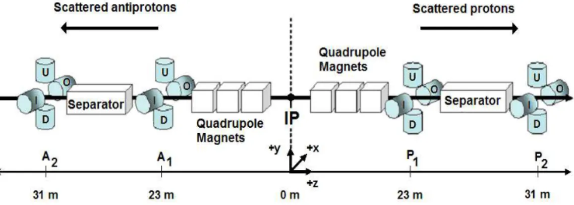
Figure 1 shows the layout of the main components of the FPD system relevant to this measurement [10]. In the center of the diagram is the interaction point, IP, at the center of the main D0 detector. A scattered proton/antiproton goes through 3 Tevatron quadrupole

magnets (with a field gradient of about 20 T/m) which alternate defocusing in the horizontal and vertical planes, passes through the first station of detectors, goes through a region free from magnetic field where electrostatic sep-arators are located, and arrives at a second station of detectors.

The FPD consists of four quadrupole spectrometers on both the scattered proton (P) and scattered antiproton (A) sides plus a dipole spectrometer (not shown). Each quadrupole spectrometer is composed of two scintillating fiber detectors, one located at about 23 m (A1 or P1) and the second at about 31 m (A2 or P2) from the IP along the Tevatron beam line. Both detectors are either above (U), below (D), on the inner side (I), or on the outer side (O) of the beam line. Given the location of the two detectors, the spectrometers on the A side are named AU, AD, AI, and AO (a similar definition is made for the P side). The pseudorapidity range covered by the detectors is about 7.3 < |η| < 8.6.

Scattered protons and antiprotons cross thin stainless steel windows at the entrance and exit of a vessel (Roman pot) containing the detectors [17]. The pots are remotely controlled and moved to within a few millimeters of the beam during stable beam conditions. The Roman pots house position detectors using 0.8 mm × 0.8 mm square double-clad polystyrene scintillating fibers to detect the passage of charged particles. Each position detector con-sists of six layers of scintillating fibers (U, U′_{, V, V}′_{, X,} X′_{), where the scintillating fibers of the U, U}′_{(V, V}′₎ lay-ers are rotated by plus (minus) 45 degrees with respect to the vertical X, X′ _{fibers (see Fig. 2).}

The fibers of the “primed” planes are offset by 0.53 mm (two-thirds of a fiber width) with respect to the fibers of the “unprimed” layers. By combining the fiber informa-tion from “primed” and “unprimed” layers, we obtain “wide” fiber segments (about 1.07 mm wide) that are used for triggering and “fine” fiber segments (about 0.27 mm wide) used for offline hit reconstruction (see Fig. 3). Each detector also contains a scintillator (read out by a time-to-digital converter system [10]) which provides a time measurement for particles passing through the de-tector with a resolution of about 1 ns. The time measure-ment is used to distinguish particles coming from the cen-ter of the D0 detector from background beam halo par-ticles (parpar-ticles traveling far enough outside of the main beam core that they pass through the FPD detector).

Beyond the active areas of the detectors, matching square clear fibers transport signals from the scintillators to 16-channel multi-anode photomultiplier tubes. The electronic signals are subsequently amplified, shaped, and sent to the D0 triggering and data acquisition system [10]. The elastic triggers are defined by the logical OR of coincident hits in all four detectors, in either of the four possible configurations of a p spectrometer and a diago-nally opposite (collinear) p spectrometer: AUPD, ADPU, AIPO, and AOPI. Several different conditions on the hits in the scintillating fiber detectors were used in the triggers: a tight (T) trigger that registered a single hit

FIG. 1: Schematic view of the Roman pot stations (A1, A2, P1, P2) comprising the forward proton detector as described in

the text (not drawn to scale). The dipole spectrometer is not shown. The letters U, D, I, O make reference to the up, down, inner and outer detectors, respectively.

FIG. 2: Schematic view of the design of one FPD scintillating fiber detector. U, U′_{, V, V}′_{, X, and X}′ _{are the scintillating}

fiber layers. The local detector x, y coordinates are indicated by the arrows. The scintillating fibers are indicated by the green stripes.

formed by the coincidence of UU′_{, VV}′_{, XX}′ _wide seg-ments; a medium (M) trigger that allowed up to three wide segments; and a loose (L) trigger that allowed hits formed from coincidences of two out of the three UU′_, VV′_{, XX}′ _{wide segments with no requirements on} num-ber of hits. To reduce backgrounds from inelastic colli-sions, LM vetoes (no hits in either the LM counters on the proton and antiproton sides) were included as part of the elastic triggers. The timing scintillator in each detector is only used for providing time information for off-line analysis and is not part of the triggers.

III. ELASTIC EVENT SELECTION

An initial data sample is obtained by requiring events to satisfy one of the elastic triggers. The p and p hit coordinates are measured in the FPD system using the fibers information and then used to select the sample of elastic scattering events. We align the detectors with

1.07 mm 0.8 mm 0.27 mm fine segment wide segment 0.53 mm 0.8 mm

U’ fiber layer U fiber layer

FIG. 3: Schematic view of part of the U and U′ _{fiber layers}

with the definitions of wide and fine fiber segments. Similar definitions are used for the X, X′ and V, V′fiber layers.

respect to the beam and then use the beam transport matrices [18] (which are functions of the currents of the magnets located between the IP and the FPD detectors and correlate the x, y coordinates and scattering angle of a particle at two specific z locations) to reconstruct the paths of protons and antiprotons through this re-gion of the Tevatron. Next, background subtraction and efficiency corrections are performed. We use a Monte Carlo (MC) event generator to apply corrections for ac-ceptance, detector resolution, beam divergence and IP size effects.

A. Data Sample

The data for this analysis were collected with dedicated beam conditions designed to facilitate the positioning of the FPD Roman pots as close to the beam axis as possi-ble. The Tevatron injection tune with the betatron func-tion of β∗ = 1.6 m at the D0 IP was used instead of the standard β∗_{= 0.35 m lattice [19]. Additionally, only} one proton bunch and one antiproton bunch were present in the Tevatron. Scraping in the vertical and horizontal

planes to remove the halo tails of the bunches was per-formed and the electrostatic separators were turned off before initiating collisions. The initial instantaneous lu-minosity was about 0.5 × 1030 _cm−2_s−1 _{with a lifetime} of about 30 hours, corresponding to a mean number of ≈ 0.8 interactions per bunch crossing. The recorded lu-minosity is about L = 31 nb−1_{, which corresponds to the} sum of two data sets used in this analysis, each with dif-ferent detector positions with respect to the beams. One set of data was taken with the closest detector position reaching about 4 mm with respect to the beam (data set 1), and the other data set was taken with detectors about 1 mm closer to the beam (data set 2). For the given instantaneous luminosity and the conditions of this store, about 33% of the elastic events are expected to be produced together with an inelastic collision in the same bunch crossing.

Approximately 20 million events were recorded using a special trigger list optimized for diffractive physics, in-cluding triggers for elastic, single diffractive, and double pomeron [20] exchange. This analysis uses elastic trig-gers, which make up about 10% of the total data col-lected. Independent triggers were used to determine effi-ciencies.

B. Hit Reconstruction

We reconstruct the proton and antiproton hits using fibers with an associated signal above the same thresh-old as used in the FPD trigger system, that is tuned to accept hits from a minimum ionizing particle. For each fiber in an un-primed layer above threshold, we verify if there is an adjacent fiber in the primed layer in order to define a “fine” fiber segment through which the particle traversed the plane. Events with more than four fibers firing in a plane are typically not due to single particles and are rejected (more than 99% of the elastic triggered events survive this condition). We require at least two out of the three UU′_{, VV}′_{, and XX}′ _{fine segments to} be reconstructed in each detector, with their intersection yielding the transverse coordinates of the hit. Since noise in some of the fibers could produce fake hits, in the case of more than one reconstructed hit in a detector (which hap-pens in about 10% of the events), we weight the hits by the sum of the analog-to-digital converter (ADC) pulse height of all the fibers that contributed to each hit and retain only the hit with the highest weight. The cor-rection for the selection efficiency, discussed in Sec. III I, accounts for elastic events discarded by this requirement. Utilizing events with fine segments in U, V, and X, we are able to estimate the offset in position and resolution within each detector by taking the difference between the x coordinate obtained from UV fiber intersection and a similar measurement using the X fiber plane. Most of the detectors used in this analysis have a resolution of about 150 µm with the exception of some of the A2 detectors that had several inactive scintillating fibers, degrading

(mm)

y

(mm)

y

DØ

a)

(mm)

y

(mm)

y

DØ

b)

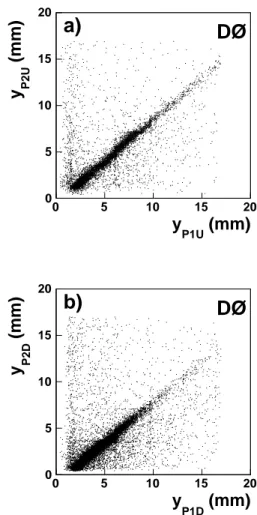
FIG. 4: Comparison of detector y coordinates in the spec-trometers a) PU and b) PD.

their resolution to about 250 µm.

C. Selection of Candidate Elastic Events

Elastic collisions produce one of the four possible hit configurations in the FPD: AUPD, ADPU, AIPO, AOPI. Since the inner and outer detectors are farther from the beam than the U and D detectors, they have poorer ac-ceptance for elastic events and are only used for align-ment purposes (see Sec. III D). If we compare the hit coordinates reconstructed by each of the two detectors of one spectrometer, we observe a correlation band from particles going through the spectrometer, but also ob-serve some uncorrelated background hits (see Fig. 4). We require hits to lie within ±3σ (σ ≈ 220 µm) from the cen-ter of the band. We decen-termine the quantity σ by fitting a Gaussian distribution obtained by projecting the hits onto an axis perpendicular to the correlation band.

We then investigate the correlation between the co-ordinates of the protons and antiprotons in diagonally

opposite spectrometers. In addition to the expected cor-relation due to the collinearity of elastic events, some background contamination due to halo particles remains. This contribution is reduced through the use of the FPD timing system, but there is still some residual back-ground, partially due to inefficiency of the trigger scintil-lators and to different acceptances of the spectrometers. A correction for the contribution from halo within the correlation band is discussed in Sec. III F.

For a specific set of p and p spectrometers in an elastic combination, we observe that elastic events with a pro-ton passing through a small region of the detectors in one spectrometer will have p positions distributed over a simi-lar but somewhat simi-larger region of the diagonally opposite spectrometer. Depending on the location of the proton, the Gaussian distribution of the p position may be trun-cated due to the finite detector size. After calculating the p acceptance correction as a function of the coordinates of the proton spectrometer, a fiducial cut is applied in the P1 detectors such that only regions in these detec-tors which require a correction of 2% or less are used. The region we select in the P1 detectors is thus guaran-teed to correspond to an acceptance greater than 98% in the other three detectors. Figure 5 shows the ypvs yp co-ordinate correlation plots (y coco-ordinate measured in the local coordinate system shown in Fig. 6), the tagging of the hits according to time-of-flight information, and the fiducial cuts applied (indicated by the dashed lines). We also check that there is no activity in the calorimeter for events in the elastic data sample. The contribution to the elastic sample from events that have a non-zero energy in the calorimeter is less than 0.1% of the total number of selected events. Most of the elastic events pro-duced in beam crossings with multiple pp interactions are suppressed by the vetoes on the LM detectors.

D. Forward Proton Detector Alignment

In order to reconstruct the tracks from the protons and antiprotons, we first align the detectors with respect to the beam and then determine the position and angle of a particle at the IP from the measured hit positions in the FPD detectors after application of the Tevatron transport matrices.

The location of the detectors with respect to the beam is determined using a sample of tracks that pass through one vertical and one horizontal detector at the same Ro-man pot station, allowing determination of the relative alignment of the detectors. We use elastic events to align one horizontal detector that did not have any overlap with the other detectors at the same z location. We de-fine the center of a vertical and a horizontal pot at each Roman pot station and then measure the positions of all four detectors with respect to this reference system. Due to the beam optics the x (y) hit coordinate distributions in the vertical proton (horizontal antiproton) detectors are narrower than in the vertical antiproton

(horizon-tal proton) detectors. Because of this effect, the offset of the beam in x for the vertical proton detectors (and the offset of the beam in y for the horizontal antiproton detectors) is determined by fitting a Gaussian distribu-tion to the x and y distribudistribu-tions in these detectors. All other beam offsets are obtained given the fact that the reconstructed IP offset and scattering angle is the same for both the proton and antiproton in an elastic event. We take the average over all four elastic combinations to determine the offset of the beam at each Roman pot station. Figure 6 shows the position of each detector ob-tained with the alignment procedure described above for the data set corresponding to the detector configuration with Roman pots located closest to the beam. The coor-dinates are plotted with respect to the beam coordinate system (dashed lines shown in the figure). For the data collected with the Roman pots retracted further away from the beam line, we use positional difference infor-mation obtained from the pot motion system added to the previously determined aligned positions. The uncer-tainty of the location of the detectors after the alignment procedure is estimated to be about 200 µm.

E. Reconstruction of p/ ¯p tracks and |t| measurement

The Tevatron transport matrices are unique for these data due to the use of the injection lattice. The beam radius (at 1σ level) ranges from 0.4 mm to 0.8 mm at the different FPD detector locations while the beam di-vergence is about 44 µrad. The change in the proton or antiproton divergence caused by the quadrupoles system is typically of the order of 1 mrad for the smallest |t| values considered in this measurement.

The size of the IP in x, y and z is typically determined by reconstructing the primary vertex using the tracking detectors [10]. Given the absence of central tracks in elas-tic events, data from non-elaselas-tic triggers, simultaneously collected with the elastic scattering events used in this analysis, are used to obtain the x, y and z distributions of the IP. The size of the IP in each direction is obtained by fitting a Gaussian function to each distribution. The measured Gaussian width of the IP distribution is about 100 µm in the transverse plane and about 45 cm along the z axis (see Fig. 7). The offsets observed in x and y from the primary vertex reconstruction are due to the fact that the center of the tracker is shifted with respect to the beam line. We use the reconstructed elastic events to determine these offsets, as described below.

To tag an elastic event, we reconstruct the coordinates of the hits in the two proton and two antiproton detec-tors. The difference of coordinates between a proton and antiproton detector yields a Gaussian distribution with a width related to the fiber offset and resolution of the two detectors, the IP size, and the beam divergence. Given the previously estimated detector resolutions and IP size, these distributions can be used to estimate the beam

(mm) AU y 0 5 10 15 20 (mm) PD y 0 5 10 15 20

No time window required DØ a) (mm) AU y 0 5 10 15 20 (mm) PD y 0 5 10 15 20

Hits in early time window DØ b) (mm) AU y 0 5 10 15 20 (mm) PD y 0 5 10 15 20

No hits in early time window DØ c) (mm) AD y 0 5 10 15 20 (mm) PU y 0 5 10 15 20

No time window required DØ d) (mm) AD y 0 5 10 15 20 (mm) PU y 0 5 10 15 20

Hits in early time window DØ e) (mm) AD y 0 5 10 15 20 (mm) PU y 0 5 10 15 20

No hits in early time window DØ f)

FIG. 5: The correlation plots ypvs ypfor the first detectors in the spectrometers (y coordinates measured in the local coordinate

system shown in Fig. 6) for AUPDand ADPU. Plots a) and d) show the correlations without any timing requirement; b) and

e) correspond to hits with a coincident tag in the corresponding scintillator early time windows; c) and f) show events with no hits within the early time window (most of the hits in this case are in the in-time window). The dashed lines correspond to the fiducial requirements applied.

x (mm) -30 -20 -10 0 10 20 30 y (mm) -30 -20 -10 0 10 20 30 1U A 1O A 1D A 1I A x (mm) -30 -20 -10 0 10 20 30 y (mm) -30 -20 -10 0 10 20 30 2U A 2O A 2D A 2I A x (mm) -30 -20 -10 0 10 20 30 y (mm) -30 -20 -10 0 10 20 30 1U P 1O P 1D P 1I P x (mm) -30 -20 -10 0 10 20 30 y (mm) -30 -20 -10 0 10 20 30 2U P 2O P 2D P 2I P

FIG. 6: Detector positions with respect to beam center (dashed lines) for the data set corresponding to the closest pot insertion to the beam. The arrows indicate the local co-ordinate system in each detector.

vergence. The values obtained are similar (40 ± 5 µrad) to those estimated using the injection tune lattice param-eters. With the coordinates of the two detectors in each spectrometer we determine the offsets of the IP (x0, y0)

(cm) IP x -0.08 -0.06 Events / cm (Normalized) 0.05 0.1 a) DØ (cm) IP y 0.18 0.2 Events / cm (Normalized) 0.05 0.1 b) DØ (cm) IP z -100 0 100 Events / cm (Normalized) 0 0.05 0.1 c) DØ

FIG. 7: Size of the IP determined by the reconstruction of the primary vertex from non-elastic triggers (black points) fitted with a Gaussian function (solid line). a) x distribution of the IP. b) y distribution of the IP. c) z distribution of the IP.

and the horizontal and vertical scattering angles (θx, θy respectively) by using the following equations:

xi = Mx,ix0+ Lx,iθx (1) yi = My,iy0+ Ly,iθy

where xi, yi are the hit coordinates in a detector i and Mx,i, Lx,i(My,i, Ly,i) are the transport matrix elements in the horizontal (vertical) axis for that detector

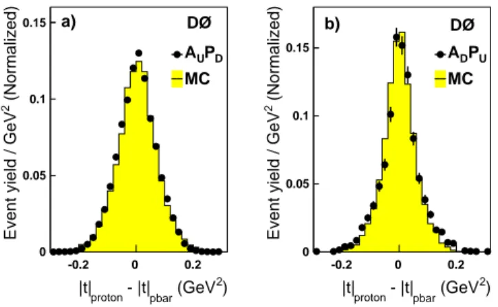
loca-) 2 (GeV pbar - |t| proton |t| -0.2 0 0.2 (Normalized) 2

Event yield / GeV

0 0.05 0.1 0.15 a) DØ D P U A MC ) 2 (GeV pbar - |t| proton |t| -0.2 0 0.2 (Normalized) 2

Event yield / GeV

0 0.05 0.1 0.15 DØ b) U P D A MC

FIG. 8: Difference in the reconstructed |t| between p and p vertical spectrometers. The MC (solid line) expected distri-bution is compared to data (solid points). a)AUPD

combina-tion. b) ADPU combination. The number of entries in each

distribution is normalized to unity.

tion. We verify that the distributions of the difference of the IP offsets and scattering angles obtained from the proton spectrometer and the antiproton spectrometer for every event are centered around zero. Since the values of θ obtained are of the order of milliradians, the four-momentum-transfer squared, t, can be approximated as

t = −p2_(θ2

x+ θ2y) (2)

where p is the momentum of the scattered particle. Given that the momenta of the elastically scattered proton and antiproton are the same as that of the incoming parti-cles (980 GeV) and that the beam momentum spread is negligibly small (0.014%) [21], the uncertainty in |t| is dominated by the measurement uncertainty of the scat-tering angle. Figure 8 shows the difference in the re-constructed |t| from the p and p vertical spectrometers, ∆|t| = |t|p− |t|p. The non-zero standard deviation of ∆|t|, σ∆t, is due to the resolution on |t|p and |t|p. The average of |t|pand |t|p(|t|ave= (|t|p+ |t|p)/2) has a reso-lution of approximately σ∆|t|/2. The |t| bin size is chosen as the largest of the observed σ∆|t| for the two detector combinations AUPD and ADPU, where the difference in σ∆|t| results from different detector resolutions. We also study the |t| resolution as a function of |t| and observe a gradual increase with |t|, from 0.02 GeV2 _{to 0.04 GeV}2_, which is reflected in the bin widths.

F. Background Subtraction

The primary source of background in the selected sam-ple is due to beam halo, consisting of either a halo pro-ton and a halo antipropro-ton in the same bunch crossing or a halo particle combined with a single diffractive event. A halo particle passing through the proton detectors in

the time window for the protons which have undergone elastic scattering usually passes through the diagonally opposite antiproton detector at an earlier time (and vice versa). Therefore, the time information can be used to veto events with early time hits, consistent with halo pro-tons and antipropro-tons in the elastic sample. The veto is not 100% efficient due to a combination of scintillator efficiency and positioning of the detectors with respect to the beam (a closer detector position both increases a detector’s signal acceptance and its ability to reject halo). Consequently, it is necessary to subtract the re-maining background. We consider an event to be caused by p (p) halo if one or both of the two p (p) detectors of an elastic combination have hits in their early time interval. We require events to have no activity in either the phalo or the phalo timing window. We select back-ground samples by requiring hits consistent with p halo and p halo simultaneously. First, we verify that outside the elastic correlation band between the coordinates of a proton and antiproton detector the signal tagged events have the same |t| dependence as the background tagged ones (see Fig. 5). Next, assuming that signal and back-ground tagged events also have the same |t| dependence inside the correlation band, we use the ratio of these two distributions and use it to estimate the percentage of background events inside the signal tagged correlation band. This background is subtracted from all events in-side the correlation band to obtain dN /dt as a function of |t|. The amount of background subtracted inside the elastic correlation band varies from 1% at low |t| to 5% at high |t|. The absolute uncertainty of the background, which is propagated as a statistical uncertainty to dσ/dt, varies from 0.3% at low |t| to 5.0% at high |t|. As a cross check, we vary the detector band cuts from 3.0σ to 3.5σ and to 6.0σ, to allow more background, and obtain sim-ilar dN /dt results after applying the same background subtraction procedure (within 1%).

G. Monte Carlo Simulation of Elastic Events

We have developed a MC generator interfaced with the Tevatron transport matrices to generate elastic events. The MC allows us to study the geometrical acceptance of the detectors, resolution of the position measurement, alignment, and effects of the beam size and beam diver-gence at the IP. The generation of events is based on an Ansatz function that we obtain by fitting the dN /dt dis-tribution of the data. We study the acceptance and bin migration effects using samples generated with a wide range of different dN /dt Ansatz distributions. The vari-ations in the corrections are included as systematic un-certainties.

The positions of hits in each detector are transformed into fiber hit information, and the reconstruction then proceeds using these hits, following the same procedure as with the data. The reconstructed correlation patterns in MC are in good agreement with those observed in data.

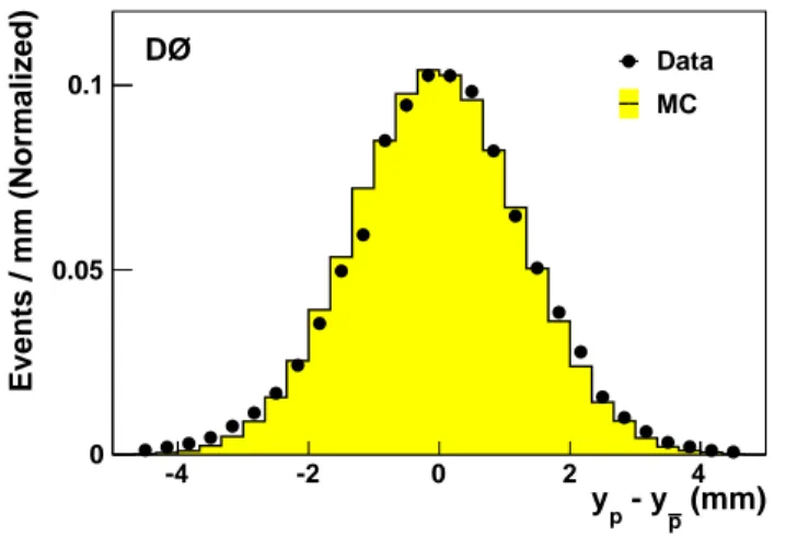
(mm) p - y p y -4 -2 0 2 4 Events / mm (Normalized) 0 0.05 0.1 Data MC DØ

FIG. 9: Comparison of MC (solid line) and data (black points) for the coordinate difference yp- ypfor the elastic

configura-tion A1,UP1,D for the data set with detectors closer to the

beam.

In addition, the MC also predicts the widths of the dif-ferent correlations as shown in Fig. 8 and Fig. 9 .

H. Acceptance and Bin Migration Correction

Due to accelerator optics, protons and antiprotons of a particular |t| are transported to an elliptical region in the x−y plane at each detector location. Each detector has a different coverage in the azimuthal angle φ and therefore a different coverage of the ellipses of constant |t|. The φ acceptance correction accounts for the fraction of the |t| ellipse for each |t| bin that is not covered by the fidu-cial area used in each detector. This correction depends only on the detector location with respect to the particle beam and on the geometry of the fiducial area used in the detector for selecting the events. Figure 10 shows the φ acceptance calculated as a function of |t| for data at the closest detector position with respect to the beam and after the fiducial cuts. We obtain similar results for the φ acceptance using the MC described in the previous sec-tion before adding the effects of beam divergence, IP size and detector resolution. The uncertainty in the φ accep-tance correction, which comes from the size of the MC sample used, is less than 0.1% at low |t| values and less than 1.0% at high |t| values. To estimate the correction for bin migration effects that is applied in data to obtain the dσ/dt distribution, we include the measured values of beam divergence, IP size, detector resolution and pot position uncertainties in the MC generator and compare to a same size MC sample with no smearing effects.

)

|t| (GeV

acceptance

φ

FIG. 10: Azimuthal acceptance of the FPD in data, after fiducial cuts, for the closest detector position of the AUPD

elastic combination. The points correspond to MC, the solid line corresponds to the calculation of the φ acceptance from the detector positions and the fiducial area.

I. Selection and Trigger Efficiencies

We simultaneously determine the effects of selection and trigger efficiencies for each of the four detectors cor-responding to an elastic configuration. To determine the efficiency of a particular detector, we use an indepen-dent trigger which does not include that detector. We obtain the dN /dt distributions with an elastic track re-constructed in the other three detectors and for all four detectors, with the trigger conditions satisfied. The ratio of the two distributions is used to extract the efficiency of the detector as a function of |t| (where |t| is reconstructed from the coordinates of the opposite side spectrometer). To avoid any additional effect from detector acceptance, we use only hits in the other three detectors in a region determined to have full geometrical acceptance in the detector of interest. We repeat a similar procedure for each of the four detectors in every elastic combination and multiply the efficiencies of the four detectors to de-termine the final efficiency correction. Typical selection and trigger efficiencies are in the range of 50% to 70% depending on the detector and trigger requirements. Ad-ditionally, we make a correction for the veto in the LM which was part of the elastic trigger. This veto filters out elastic events that are produced in coincidence with an inelastic collision in the same bunch crossing (pileup). To make this correction, we use a trigger based on hits in the proton spectrometers with no LM requirement and determine the fraction of candidate elastic events recon-structed in coincidence with the LM. We find that about 27% (20%) of elastic events for data set 1 (2) as defined in Sec. III A were removed by the LM veto.

J. Luminosity

Since elastic data were collected with Tevatron con-ditions modified with respect to standard operations of the D0 experiment, we compare the number of inclusive jet events obtained from our data to the number of jet events used for the inclusive cross section measurement discussed in [22] to determine the integrated luminosity. The corresponding integrated luminosity for data set 1 (2) is 18.3 nb−1_{(12.6 nb}−1_{), with an uncertainty of 13%.} We add in quadrature the uncertainty in the standard lu-minosity determination (6.1% [23]) and obtain an overall normalization uncertainty of 14.4%.

IV. SYSTEMATIC UNCERTAINTIES

The major |t|-dependent contributions to the system-atic uncertainties in the measurement of dσ/dt are due to detector efficiencies, beam divergence, detector posi-tions, and the choice of the Ansatz function. The lumi-nosity measurement contributes to the overall normaliza-tion uncertainty. The Tevatron beam transport matrices are known with high precision (within 0.1%) and there-fore produce a small uncertainty in our results compared to the other sources. We take the uncertainty in the posi-tion of the pot from the beam center as an extra “smear-ing” factor for the hit coordinates in the MC. Since the efficiencies vary with |t|, we fit either a polynomial or an exponential function to each trigger efficiency and prop-agate the uncertainties in the fit parameters to dσ/dt, using the covariance matrix of the fit. For the beam di-vergence term, we vary the beam didi-vergence by ±5 µrad in the MC, and we propagate the change in the accep-tance correction bin-by-bin to dσ/dt. We also consider 26 possible variations of the Ansatz function used in the MC to account for the uncertainties in the logarithmic slopes before and after the kink and also for the |t| value where the kink is observed.

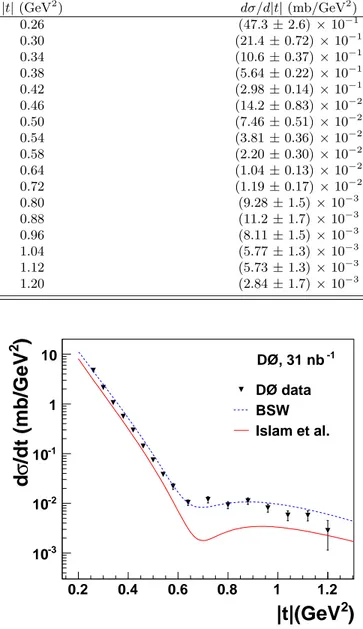
V. RESULTS

In total, we have four independent measurements of dσ/dt that come from the two elastic combinations (AUPDand ADPU) and two data sets, which agree with each other within the uncertainties. We combine the four measurements using a bin-by-bin weighted average. The resulting values for the dσ/dt distribution, together with their total uncertainties, are listed in Table I and shown in Fig. 11. The uncertainties are the total experimen-tal uncertainties excluding the 14.4% normalization un-certainty. The |t| bin centers are determined using the prescription described in [24], however, the values found are very close to the middle of the bin. Two phenomeno-logical model predictions for√s = 1.96 TeV (BSW [25], Islam et al. [26]) are also shown. The BSW model shows a good description of the data in shape and normalization

TABLE I: The dσ/dt differential cross section. The statistical and systematic uncertainties are added in quadrature. The luminosity uncertainty of 14.4% is not included.

|t| (GeV2₎ dσ/d|t| (mb/GeV2₎ 0.26 (47.3 ± 2.6) × 10−1 0.30 (21.4 ± 0.72) × 10−1 0.34 (10.6 ± 0.37) × 10−1 0.38 (5.64 ± 0.22) × 10−1 0.42 (2.98 ± 0.14) × 10−1 0.46 (14.2 ± 0.83) × 10−2 0.50 (7.46 ± 0.51) × 10−2 0.54 (3.81 ± 0.36) × 10−2 0.58 (2.20 ± 0.30) × 10−2 0.64 (1.04 ± 0.13) × 10−2 0.72 (1.19 ± 0.17) × 10−2 0.80 (9.28 ± 1.5) × 10−3 0.88 (11.2 ± 1.7) × 10−3 0.96 (8.11 ± 1.5) × 10−3 1.04 (5.77 ± 1.3) × 10−3 1.12 (5.73 ± 1.3) × 10−3 1.20 (2.84 ± 1.7) × 10−3

)

|t|(GeV

)

/dt (mb/GeV

σ

d

FIG. 11: The measured dσ/dt differential cross section. The normalization uncertainty of 14.4% is not shown. The uncer-tainties are obtained by adding in quadrature statistical and systematic uncertainties. The predictions of BSW ([25]) and Islam et al. ([26]) are compared to the data.

and is able to reproduce the kink within experimental uncertainties.

The |t| range covered by our measurement is 0.26 < |t| < 1.2 GeV2_{. We observe a change in} the logarithmic slope of the dσ/dt distribution at |t| ≈ 0.6 GeV2_{. A fit to the dσ/dt distribution in} the range 0.26 < |t| < 0.6 with an exponential func-tion of the form Ae−b|t| _{yields a logarithmic slope} pa-rameter of b = 16.86 ± 0.10 (stat) ± 0.20 (syst) GeV−2

)

|t|(GeV

)

/dt (mb/GeV

σ

d

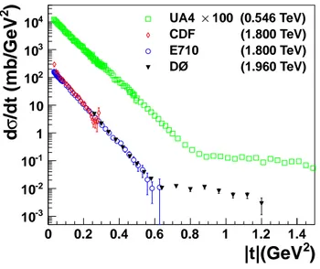
FIG. 12: The dσ/dt differential cross section measured by the D0 Collaboration and compared to the CDF and E710 mea-surements at√s = 1.8 TeV, and to the UA4 measurement at √_{s = 0.546 TeV (scaled by a factor of 100). A normalization} uncertainty of 14.4% on the D0 measurement is not shown.

(χ2_{= 6.63 for 7 degrees of freedom).}

Figure 12 shows a comparison of our results to those obtained at √s = 1.8 TeV by the CDF and E710 Teva-tron Collaborations [11, 12], and also to that of the UA4 Collaboration at√s = 0.546 TeV [27]. Our measurement of the slope parameter agrees within uncertainties with previous measurements by the CDF (b = 16.98 ± 0.25 GeV−2_{) and E710 (b = 16.30 ± 0.30 GeV}−2₎

Collabora-tions. A comparison of the shape of our measured dσ/dt to UA4 measurement shows that the kink in dσ/dt moves towards lower |t| values as the energy is increased, but, as in the UA4 data, we do not see a distinct minimum as observed in pp elastic interactions ([13]).

In summary, we have presented the first measurement of dσ(pp→ pp)/dt as a function of |t| at√s = 1.96 TeV. Our measurement extends the |t| and √s range previ-ously studied and shows a change in the |t| dependence, consistent with the features expected for the transition between two diffractive regimes.

VI. ACKNOWLEDGEMENTS

We thank the Fermilab Beams Division for designing and providing the special beam conditions for the data taking. In particular we thank N. Mokhov, S. Drozhdin, M. Martens and A. Valishev for their important contri-butions to the FPD. We also thank J. Soffer and M. Islam for useful discussions.

We thank the staffs at Fermilab and collaborating institutions, and acknowledge support from the DOE and NSF (USA); CEA and CNRS/IN2P3 (France); MON, Rosatom and RFBR (Russia); CNPq, FAPERJ, FAPESP and FUNDUNESP (Brazil); DAE and DST (In-dia); Colciencias (Colombia); CONACyT (Mexico); NRF (Korea); FOM (The Netherlands); STFC and the Royal Society (United Kingdom); MSMT and GACR (Czech Republic); BMBF and DFG (Germany); SFI (Ireland); The Swedish Research Council (Sweden); and CAS and CNSF (China).

[1] t = (pf − pi)2 where pi and pf are the initial and final

particles four-momenta, respectively. [2] M. Block, Phys. Rep. 436, 71 (2006). [3] G. Giacomelli, Phys. Rep. 23, 123 (1976). [4] G. Alberi and G. Goggi, Phys. Rep. 74, 1 (1981). [5] A. Breakstone et al., Phys. Rev. Lett. 54 2180 (1985). [6] E. Nagy et al.(CHHOV Collaboration), Nucl. Phys. B

150, 221 (1979).

[7] V. Barone and E.Predazzi, High Energy Particle Diffrac-tion (Springer-Verlag, Berlin, 2002).

[8] A. Donnachie, P. Landshoff, Nucl. Phys. B 387, 637 (1996).

[9] J. Forshaw and D.A. Ross, Quantum Chromodynamics and the Pomeron (Cambridge University Press, Cam-bridge, 1997).

[10] V. M. Abazov et al. (D0 Collaboration), Nucl. Instr. Meth. Phys. Res. A 565, 463 (2006).

[11] F. Abe et al. (CDF Collaboration), Phys. Rev. D 50, 5518 (1994).

[12] N. Amos et al. (E710 Collaboration), Phys. Lett. B 247, 127 (1990).

[13] G. Antchev et al.(TOTEM Collaboration), Eur. Phys. Lett. 95, 41001 (2011).

[14] The pseudorapidity is defined as η = − ln[tan(θ/2)], where θ is the polar angle with respect to the proton beam direction.

[15] S. Abachi et al. (D0 Collaboration), Nucl. Instr. Meth. Phys. Res. A 338, 185 (1994).

[16] V. M. Abazov et al. (D0 Collaboration), Nucl. Instr. Meth. Phys. Res. A 552, 372 (2005).

[17] U. Amaldi et al., Phys. Lett. B 44, 112 (1973).

[18] M. G. Minty and F. Zimmerman, Measurement and Con-trol of Charged Particle Beams (Springer-Verlag, Berlin, 2003).

[19] S. D. Holmes, FERMILAB-TM-2484 (1998).

[20] V. M. Abazov et al. (D0 Collaboration), Phys. Lett. B 705, 193 (2011).

[21] J. Stogin, T. Sen and R.S. Moore, JINST 7, T01001 (2012).

[22] V. M. Abazov et al. (D0 Collaboration), Phys. Rev. Lett. 101, 062001 (2008).

[23] T. Andeen et al., FERMILAB-TM-2365 (2007).

[24] G. Laferty and T. Wyatt, Nucl. Instr. Meth. Phys. Res. A 355, 541 (1995).

[25] C. Bourrely, J. Soffer, and T.T. Wu, Eur. J. Phys. C 28, 97 (2003).

[26] M. M. Islam, J. Kaspar, R. J. Luddy, and A. V. Prokudin, in Proceedings of the 13th _{International Conference on}

Elastic and Diffractive Scattering, CERN, Geneva, June-July 2006, arXiv:1002.3527 [hep-ph].

[27] M. Bozzo et al. (UA4 Collaboration), Phys. Lett. B 155, 197 (1985).