The accretion process in neutron-star low-mass X-ray binaries

The Accretion Process in Neutron-star Low-mass X-ray

Binaries

by

Dacheng Lin

B.S., University of Science and Technology of China (2003) Submitted to the Department of Physics

in partial fulfillment of the requirements for the degree of Doctor of Philosophy

at the

MASSACHUSETTS INSTITUTE OF TECHNOLOGY September 2009

c

Dacheng Lin, MMIX. All rights reserved.

The author hereby grants to MIT permission to reproduce and distribute publicly paper and electronic copies of this thesis document in whole or in part.

Author . . . . Department of Physics

July 27, 2009

Certified by . . . . Ronald A. Remillard Principal Research Scientist Thesis Supervisor Certified by . . . . Deepto Chakrabarty Professor of Physics Thesis Co-supervisor Accepted by . . . . Thomas J. Greytak Lester Wolfe Professor of Physics Associate Department Head for Education

The Accretion Process in Neutron-star Low-mass X-ray Binaries by

Dacheng Lin

Submitted to the Department of Physics on July 27, 2009, in partial fulfillment of the

requirements for the degree of Doctor of Philosophy

Abstract

There had been long-standing fundamental problems in the spectral studies of accreting neutron stars (NSs) in low-mass X-ray binaries involving the X-ray spectral decomposition, the relations between subtypes (mainly atoll and Z sources), and the origins of different X-ray states. Atoll sources are less luminous and have both hard and soft spectral states, while Z sources have three distinct branches (horizontal(HB)/normal(NB)/flaring(FB)) whose spectra are mostly soft.

I analyzed more than twelve-year RXTE observations (∼ 2500 in total) of four atoll sources Aql X–1, 4U 1608–522, 4U 1705–44, and 4U 1636–536. I developed a hybrid spec-tral model for accreting NSs. In this model, atoll hard-state spectra are described by a single-temperature blackbody (BB), presumed to model emission from the boundary layer where the accreted material impacts the NS surface, and a strong Comptonized compo-nent, modeled by a cutoffpl power law (CPL). Atoll soft-state spectra are described by two thermal components, i.e., a multicolor disk (MCD) and a BB, with additional weak Comp-tonized component, modeled by a single power law. I found that the accretion disk in most of the soft state is truncated at a constant value, most probably at the innermost stable circular orbit (ISCO), predicted by general relativity. This allows us to derive upper limits of magnetic fields on the NS surface of the above four atoll sources. The apparent emission area of the boundary layer is small, ∼1/16 of the whole NS surface, but is fairly constant, spanning the hard and soft states. All this was not seen if the classical models for thermal emission plus high Comptonization were used instead. By tracking the accretion rate onto the NS surface, I inferred a strong mass jet in the hard state. My study of 4U 1705–44 using broadband spectra from Suzaku and BeppoSAX supported the above results.

From my spectral study of the above four atoll sources, I also found that in a part of the soft state with frequent occurrences of kilohertz quasi-periodic oscillations (kHz QPOs), the accretion disk appears to be truncated at larger radii than in other parts of the soft state where the disk is presumably truncated at the ISCO. Thus the production of kHz QPOs in accreting NSs should be closely related to the behavior of the accretion disk. It is well known that the kHz QPO amplitude spectrum tracks the BB, even though we see no changes in the BB spectral evolution track when kHz QPOs are present. The simplest interpretation is that accretion oscillations are imparted in the inner disk and then seen as the waves impact the NS surface in the boundary layer.

The transient XTE J1701-462 (2006-2007) is the only source known to exhibit properties of both the Z and atoll types. I carried out the state/branch classifications of all the ∼900 RXTE observations. The Z-source branches evolved substantially in the X-ray color-color diagram during this outburst. In the decay, the HB, NB and FB disappeared successively, with the NB/FB transition evolving to the atoll-source soft state. Spectral analyses using my new spectral model show that the inner disk radius maintains at a nearly constant

value, presumably at ISCO, when the source behaves as an atoll source in the soft state, but increases with accretion rates when the source behaves as a Z source at high luminosity. We interpreted this as local Eddington limit effects and advection domination in the accretion disk. The disks in the two Z vertices probably represent two stable accretion configurations, and we speculate that the lower (NB/FB) vertex represents a standard thin disk and the upper (HB/NB) vertex a slim disk. The changes in the accretion rate are responsible for movement of Z-source branches and the evolution from one source type to another. However, the three Z-source branches are caused by three mechanisms that operate at a roughly constant accretion rate. The FB is an instability tied to the Eddington limit. It is formed as the inner disk radius temporarily decreases toward the ISCO. The NB is traced out mostly due to changes in the boundary layer emission area, as a result of the system transiting from a standard thin disk to a slim disk. The HB is formed with the increase in Comptonization, consistent with strong radio emission detected from this branch.

Thesis Supervisor: Ronald A. Remillard Title: Principal Research Scientist

Thesis Co-supervisor: Deepto Chakrabarty Title: Professor of Physics

Acknowledgments

It is the most worthwhile journey to have written this work, during which I harvest knowl-edge, love, and friendship, and eventually reach this milestone of my life. Here I would like to make the acknowledgments to my mentors, colleagues, friends, and family, without whom, this thesis would be impossible.

First, I would like to express my deepest appreciation to my advisor, Ronald A. Remil-lard. His help includes many aspects, and the impact on my life is invaluable. It is not often that one finds an advisor who not only always finds time to give expert guidance to research projects but also care about his common life, including learning of English and understanding of American culture, which is essential for me, an international student here in the United States. I am also indebted to other MIT RXTE group members, i.e., Hale V. Bradt, Alan M. Levine, and Edward H. Morgan, for their great help.

Second, my special thanks go to Jeroen Homan, who is my another constant collabo-rator at MIT. He has made his support available in a number of ways. There are also a lot of other collaborators who I would like to show my gratitude to. They include Jeffrey E. McClintock and Ramesh Narayan and other members in their group at Harvard CFA, Diego Altamirano, Tomaso M. Belloni, Rudy Wijnands, etc. I would also like to thank my thesis committee members Deepto Chakrabarty, Saul A. Rappaport, and Joshua N. Winn for their instructions during my preparation for this thesis.

Also, I would like to thank all astrograds, both former and current, for the help and happiness they brought to me in the past six years. They include Lindy Blackburn, Jeff Blackburne, Ben Cain, Josh Carter, Aidan Crook, Tamer Elkholy, Will Farr, Joel Fridriks-son, Jake Hartman, Miriam Krauss, Ryan Lang, Adrian Liu, Ying Liu, Jinrong Lin, Jared Markowitz, Michael Matejek, Madhusudhan Nikku, En-Hsin Peng, Leslie Rogers, Robyn Sanderson, Leo Stein, Michael Stevens, Pranesh Adhyan Sundararajan, Molly Swanson, Sarah Vigeland, Chris Williams, and Philip Zukin. Several current and past post-doctors, such as Li Ji and Yangsen Yao, also help me a lot. Thank you.

In addition, I thank a lot of friends, from those who share their happiness in common life with me to those in the Ashdown House Executive Committee and the MIT Graduate Student Council in the same year as me. I learned a lot from them.

Last, but not the least, I have many thanks to my family. In particular, I thank my wife, Yaning Li, for her incredible support and love. I also thank my mother, brothers, sister and sisters-in-law for their long-term understanding, support and love.

Contents

List of Figures 14

List of Tables 15

1 Introduction 17

1.1 X-ray binary systems . . . 17

1.2 Physics in X-ray binaries: why we study them . . . 20

1.3 Techniques used to study X-ray binaries . . . 26

1.4 BH and NS X-ray binaries . . . 27

1.5 Weakly magnetized NS LMXBs . . . 28

1.6 Organization and content of thesis . . . 29

2 X-ray Observatory and Data Analyses 31 2.1 The Rossi X-ray Timing Explorer . . . 31

2.1.1 Instruments . . . 31 2.1.2 Data Analyses . . . 33 2.2 Suzaku . . . 34 2.2.1 Instruments . . . 36 2.2.2 Data Analyses . . . 37 2.3 BeppoSAX. . . 38 2.3.1 Instruments . . . 38 2.3.2 Data Analyses . . . 39

3 Accretion Physics and X-ray Emission Mechanisms 41 3.1 Accretion physics . . . 41

3.1.1 Spherically symmetric accretion and Eddington luminosity . . . 41

3.1.2 The standard thin disk . . . 44

3.1.3 The magnetorotational instability . . . 46

3.1.4 Local Eddington limit in the accretion disk . . . 46

3.1.5 Accretion timescales . . . 47

3.1.6 The relativistic accretion disk . . . 48

3.1.7 ADAF and slim disk . . . 48

3.1.8 The boundary layer . . . 49

3.2 X-ray emission mechanisms . . . 51

3.2.1 Blackbody radiation and multicolor disk blackbody . . . 51

3.2.2 Inverse Compton Scattering . . . 55

3.2.3 Bremsstrahlung . . . 55

4 Evaluating Spectral Models and the X-ray States of Neutron-Star X-ray

Transients 57

4.1 Introduction . . . 57

4.2 Observations and data reduction . . . 59

4.3 Light curves and color-color diagrams . . . 60

4.4 Spectral modeling . . . 64

4.4.1 Spectral models and assumptions . . . 64

4.4.2 Comptonized + thermal two-component models . . . 65

4.4.3 Double thermal models . . . 74

4.5 Timing properties and comparison with black holes . . . 76

4.6 Physical interpretations of model 6 for thermal components . . . 78

4.7 Physical consequences of model 6 for the hard state . . . 80

4.8 Summary and discussion . . . 82

5 Suzaku and BeppoSAX X-ray Spectra of the Persistently Accreting Neutron-Star Binary 4U 1705-44 85 5.1 Introduction . . . 85

5.2 Observations and data reduction . . . 87

5.2.1 Suzaku data . . . 88

5.2.2 BeppoSAX data . . . 91

5.3 Spectral modeling . . . 93

5.3.1 Spectral models and assumptions . . . 93

5.3.2 Spectral fit results . . . 95

5.3.3 Relativistic Fe lines . . . 100

5.4 Discussion . . . 103

5.4.1 Inner disk radius . . . 103

5.4.2 Constraint on the magnetic field in 4U 1705–44 . . . 104

5.4.3 The boundary layer . . . 104

5.5 Conclusion . . . 106

6 Spectral Study of Accreting Neutron-Star X-ray Sources and Hint on Origins of Kilohertz Quasi-periodic Oscillations 107 6.1 Introduction . . . 108

6.2 Observations and data reduction . . . 109

6.3 Light curves and color-color diagrams . . . 110

6.4 Spectral variability . . . 113

6.5 Kilohertz quasi-periodic oscillations . . . 116

6.6 Spectral modeling . . . 116

6.6.1 Spectral models and assumptions . . . 116

6.6.2 Spectral fit results . . . 118

6.7 Timing properties and comparison with spectral fit results . . . 124

6.7.1 Rapid variability and Comptonization . . . 124

6.7.2 Kilohertz quasi-periodic oscillations in the lower left banana . . . 125

7 Spectral States of XTE J1701-462: Link between Z and Atoll Sources 127

7.1 Introduction . . . 127

7.2 Observations and data reduction . . . 133

7.3 Light curves and color-color diagrams . . . 134

7.3.1 Source state/branch classification . . . 134

7.3.2 Source evolution and relations between source types . . . 138

7.3.3 Evolution speed along branches . . . 139

7.3.4 Selection of spectra for spectral fits . . . 142

7.4 Spectral modeling . . . 146

7.4.1 Spectral models and assumptions . . . 146

7.4.2 Atoll source stage . . . 149

7.4.3 Z Source Stages . . . 150

7.5 Broadband variability . . . 157

7.6 Discussion . . . 158

7.6.1 Secular evolution of XTE J1701-462 and the role of ˙m . . . 158

7.6.2 Physical processes along the Z branches of XTE J1701–462 . . . 161

7.6.3 Comparison with other NS LMXBs . . . 163

7.7 Conclusions . . . 163

8 Type I X-ray Bursts from the Neutron-star Transient XTE J1701-462 167 8.1 Introduction . . . 167

8.2 Observations and burst search . . . 168

8.3 Burst spectral fits . . . 171

8.4 Burst oscillation search . . . 173

8.5 Discussions and conclusions . . . 173

9 Spectral Properties of GX 17+2 177 9.1 Introduction . . . 177

9.2 Observations and color-color diagrams . . . 178

9.3 Spectral modeling . . . 182

9.4 Conclusions and discussions . . . 185

10 Physical Interpretations of Accretion in NS LMXBs 187 10.1 Brief summary of results of this thesis . . . 187

10.2 Detailed summary of the spectral study results . . . 188

10.2.1 Color-color and hardness-intensity diagrams . . . 188

10.2.2 Summary of spectral fit results . . . 192

10.3 Physical interpretations derived from spectral analyses . . . 199

10.3.1 A new spectral model for weakly magnetized NS LMXBs . . . 199

10.3.2 The accretion disk inner radius and the boundary layer effective area in atoll sources . . . 199

10.3.3 NS radius vs. the ISCO in atoll sources . . . 199

10.3.4 Magnetic fields of the NS in atoll sources . . . 200

10.3.5 Investigation of kilohertz quasi-periodic oscillations in atoll sources . 201 10.3.6 Relation between source types and the role of mass accretion rates . 202 10.3.7 Accretion disk and boundary layer in Z sources and the Eddington limit . . . 202 10.3.8 Speculations for different disk solutions for the vertices of Z sources 203

10.3.9 The physical nature of different branches in Z sources . . . 203

List of Figures

1-1 Artist’s impression of a low-mass X-ray binary . . . 18

1-2 The X-ray long-term light curves of seven NS X-ray binaries . . . 19

1-3 The sample CDs and HIDs of NS X-ray binaries . . . 21

1-4 The sample unfolded energy spectra and power density spectra of the BH X-ray binary GRO J1655–40 in different X-ray spectral states . . . 22

1-5 The sample unfolded energy spectra and power density spectra of the atoll type NS 4U 1636–536 in different X-ray spectral states . . . 23

1-6 The sample unfolded energy spectra and power density spectra of pulsars SAX J1808.4–3658 and V 0332+53 . . . 24

1-7 The sample unfolded energy spectra and power density spectra of the Z source GX 17+2 in different X-ray spectral branches . . . 25

2-1 Diagram of the RXTE spacecraft . . . 32

2-2 Diagram of the Suzaku spacecraft . . . 35

2-3 Diagram of the BeppoSAX spacecraft . . . 38

3-1 The main X-ray emission components in weakly magnetized NS LMXBs. . . 42

3-2 Luminosity versus inner disk temperature for the BH X-ray binaries . . . . 52

3-3 Comparison between two XSPEC thermal disk models DISKBB and DISK 53 3-4 Comparison of DISKBB with relativistic disk models BHSPEC and KERRBB 53 4-1 Long-term light and color curves of Aql X–1 and 4U 1608–52 . . . 61

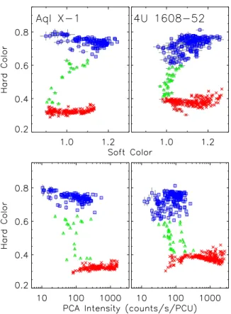
4-2 Normalized color-color and color-intensity diagrams of Aql X–1 and 4U 1608–52 62 4-3 The HEXTE intensity in two hard energy bands versus the PCA intensity at 3–20 keV for Aql X–1 and 4U 1608–52 . . . 63

4-4 The unfolded spectra and residuals of two sample observations of Aql X–1 using different kinds of models . . . 66

4-5 The unfolded spectra and residuals of two sample observations of Aql X–1 with best-fitting kTs&1 keV using Model CompTT+MCD (hot-seed-photon model) . . . 67

4-6 Variation of the temperature of the thermal component with the PCA inten-sity for Aql X–1 and 4U 1608–522 . . . 70

4-7 The luminosity of the thermal component versus its characteristic tempera-ture for Aql X–1 and 4U 1608–522 . . . 71

4-8 The luminosity of the Comptonized component versus the luminosity of the thermal component(s) for Aql X–1 and 4U 1608–522 . . . 72

4-9 The unfolded spectra and residuals of two sample soft-state observations of Aql X–1 using model MCD+BB+CBPL . . . 74

4-10 The fraction of Comptonized luminosity versus the total luminosity for Aql X– 1 . . . 74 4-11 The integrated rms power in the power density spectrum for Aql X–1 and

4U 1608–52 . . . 76 4-12 The integrated rms power versus the fraction of luminosity contained in the

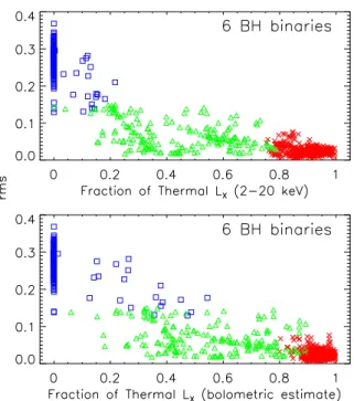
thermal (MCD) component for 6 black hole systems. . . 77 4-13 The rms power versus the fraction of luminosity contained in BB and/or

MCD components as evaluated for different spectral models for Aql X–1 and 4U 1608–52 . . . 77 4-14 The luminosity evolution of different spectral components (middle panel)

during the 2000 outburst of Aql X–1, as viewed with Model 6 . . . 80 4-15 The luminosity of non-BB components (i.e., BPL+MCD) versus the

lumi-nosity of the BB component for Aql X–1 and 4U 1608–522 . . . 81 5-1 The long-term light curve of 4U 1705–44 . . . 87 5-2 Color-color and hardness-intensity diagrams of 4U 1705–44 based on Suzaku

observations in 2006–2008 . . . 88 5-3 Example of unfolded spectra at different states using different models for

4U 1705–44 . . . 92 5-4 The luminosity of the thermal components versus their characteristic

tem-peratures for 4U 1705–44 . . . 95 5-5 The energy fraction of Comptonized luminosity versus the total luminosity,

from model MCD+BB+PL for 4U 1705–44 . . . 96 5-6 The luminosity of the MCD component plus Comptonization versus the BB

luminosity for 4U 1705–44 . . . 96 5-7 Fe lines from 4U 1705–44, fit by the diskline model . . . 101 5-8 The variation of the equivalent width of the Fe lines with the source

lu-minosity, for soft-state data only. The continuum spectra are fit by model MCD+BB+PL, and model SIMPL(MCD)+BB gives quite similar results. 102 5-9 The variation of the equivalent width of the Fe lines with the source

lumi-nosity for 4U 1705–44 . . . 102 6-1 Long-term light and color curves of Aql X–1, 4U 1608-522, 4U 1705–44 and

4U 1636–536. . . 111 6-2 Color-color and hardness-intensity diagrams of atoll sources . . . 112 6-3 The HEXTE intensity in two hard energy bands versus the PCA intensity

for atoll sources . . . 112 6-4 Fractional spectral variations for atoll source based on count rates . . . 114 6-5 Fractional spectral variations for atoll sources based on colors . . . 115 6-6 The luminosity of the thermal components versus their characteristic

tem-peratures for atoll sources . . . 119 6-7 The apparent inner disk radius and size of the boundary layer for atoll sources120 6-8 The apparent inner disk radius and size of the boundary layer for atoll sources120 6-9 The power-law index and cutoff energy of the cutoff power-law in the fit of

atoll-source hard state . . . 121 6-10 The fraction of Comptonized luminosity versus the total luminosity for atoll

6-11 The fraction of Comptonized luminosity versus the total luminosity for atoll sources . . . 122 6-12 The integrated rms power versus the hard color for atoll sources . . . 124 6-13 The rms versus the fraction of luminosity contained in BB and/or MCD

components for atoll sources . . . 125 7-1 CDs and HIDs of the Cyg-like Z source GX 340+0 (MJD 51920–51925) and

the Sco-like Z source GX 17+2 (MJD 51454–51464) . . . 128 7-2 PCA spectra of GX 340+0 and GX 17+2 from key positions along their Z

tracks . . . 129 7-3 The RXTE ASM one-day-averaged light curve of XTE J1701–462 during its

2006–2007 outburst and the RXTE PCA 32-s luminosity curve . . . 130 7-4 RXTE PCA 32-s light curves of XTE J1701–462 in two energy bands during

the 2006–2007 outburst . . . 134 7-5 The CDs and HIDs for the five stages of the outburst for XTE J1701–462 . 135 7-6 The complete HID of the 2006–2007 outburst of XTE J1701–462 . . . 136 7-7 The evolution speed of XTE J1701–462 along the flaring branch . . . 140 7-8 The evolution speed of XTE J1701–462 along the normal branch . . . 140 7-9 Different measures of spectral variability during the Z stages of XTE J1701–462143 7-10 Light curves, CDs and HIDs of the sample intervals from XTE J1701–462 . 144 7-11 Comparison of the PCA spectra of XTE J1701-462 in key positions along the

Z tracks . . . 145 7-12 The fraction of the LCBPL with one-σ error bars for XTE J1701–462 . . . . 147

7-13 Examples of unfolded spectra at different states/branches for XTE J1701–462 148 7-14 Spectral fitting results for the atoll stage of the outburst for XTE J1701–462 150 7-15 The spectral fitting results for the sample intervals for XTE J1701–462 . . . 151 7-16 The spectral fitting results for the whole Z stage of XTE J1701–462 . . . . 152 7-17 The emission sizes of the thermal components versus the total LX for the

NB/FB vertex and the atoll source stage of XTE J1701–462 . . . 153 7-18 The difference of spectra for the two ends of the NB during interval IIIa for

XTE J1701–462 . . . 155 7-19 The emission sizes of the thermal components versus the total LX for the

HB/NB vertex for XTE J1701–462 . . . 156 7-20 The fractions of the LMCD and LMCD+CBPL on the HB and the HB/NB

vertex for XTE J1701–462 . . . 157 7-21 The rms of XTE J1701–462 for its 2006–2007 outburst . . . 158 8-1 The one-day ASM light curve and 32-s PCA light curve of XTE J1701–462 169 8-2 The color-color and hardness-intensity diagrams for observations between

MJD 54260 and 54315 in the decay of the 2006-2007 outburst of XTE J1701–462170 8-3 The results of the spectral fits of time-resolved spectra of the three bursts

detected from XTE J1701-462 during its 2006-2007 outburst . . . 171 8-4 The burst luminosity versus blackbody temperature for the three bursts from

XTE J1701–462 . . . 172 9-1 RXTE ASM one-day-averaged light curves of GX 17+2 spanning ∼12 years 179 9-2 RXTE PCA 32-s light curves of GX 17+2 during MJD 51454.1–51463.3 in

9-3 The color-color and hardness-intensity diagrams for observations of GX 17+2

between MJD 51454 and 51464 . . . 180

9-4 The ratios of the spectra on the two ends of each branch of GX 17+2 . . . 181

9-5 The results of the spectral fit of Sz-resolved spectra for GX 17+2 . . . 183

9-6 The results of the spectral fit of Sz-resolved spectra as a function of the rank number Sz for GX 17+2 . . . 184

10-1 Color-color and hardness-intensity diagrams of atoll sources . . . 189

10-2 Color-color and hardness-intensity diagrams of Z sources . . . 189

10-3 Color-color and hardness-intensity diagrams of the transient Z source XTE J1701– 462 in three time intervals . . . 190

10-4 The hardness-intensity diagram of the transient Z source XTE J1701–462 from its 2006–2007 outburst . . . 191

10-5 Source evolution in the hardness-intensity diagram. . . 191

10-6 Example of unfolded spectra at different states using different models . . . 193

10-7 Spectral fit results of atoll sources . . . 194

10-8 Fit results of broad-band spectra of 4U 1705–44 observed by Suzaku and BeppoSAX. . . 195

10-9 Spectral fit results of transient source XTE J1701–462 . . . 196

10-10Fit results of Z source GX 17+2. . . 196

List of Tables

4.1 X-ray Sources and Observations Prior to 2006 January 1 . . . 60

4.2 The spectral models . . . 64

4.3 Best-fitting parameters of two sample spectra . . . 65

5.1 The Suzaku observations of 4U 1705–44 in 2006–2008 . . . 88

5.2 The BeppoSAX observations of 4U 1705–44 . . . 91

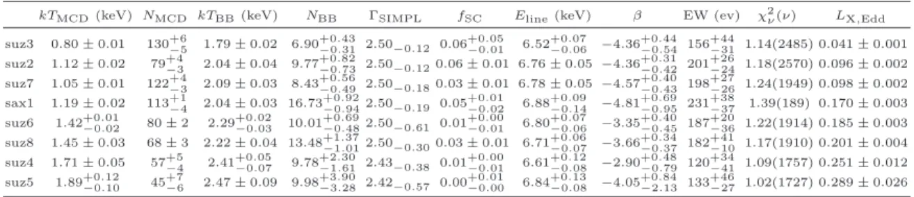
5.3 Spectral modeling results of soft-state observations using MCD+BB+PL+diskline 97 5.4 Spectral modeling results of soft-state observations using SIMPL(MCD)+BB+diskline 97 5.5 Spectral modeling results of hard-state observations using BB+CPL+diskline 97 6.1 Observations and State Definitions for Each Source . . . 110

6.2 Physical Parameters Assumed in Spectral Study . . . 117

7.1 Statistics for observation time of the source in different states/branches . . 138

Chapter 1

Introduction

This thesis is dedicated to the study of accretion physics in low-mass X-ray binaries (LMXBs), in which a neutron star (NS) or a stellar-mass black hole (BH) accretes matter from a low-mass companion star through an accretion disk. Intense X-ray emission is released from the inner accretion disk and/or the boundary layer produced by impact of the accretion flow on the NS surface. LMXBs are important cosmic laboratories for studying the properties of strong gravitational fields and dense matter. X-ray spectral studies of the BHs are in an advanced stage, e.g., spin parameters have been derived from relativistic accretion disk models for several BHs [e.g., Shafee et al., 2006]. NS binaries show many spectral differ-ences from the BHs, and their spectral studies can provide additional valuable information on accretion processes and the nature of the NSs. However, progress had been impeded by the long-standing ambiguity about the spectral decomposition for the NSs. The work of this thesis devises a new way to model the spectra of weakly magnetized bright NS LMXBs, and offers new physical interpretations of spectral evolution of different subclasses.

In this introduction, I will first describe the general properties of X-ray binaries in §1.1. I then describe different classes of LMXBs.

1.1

X-ray binary systems

A normal star is supported against its strong gravity by pressure of interior hot gas heated by nuclear burning. As all the nuclear energy is exhausted, it has to collapse to a much denser state. The end product is a compact object, which can be a white dwarf (WD), a NS or a BH, depending on the mass (M ). A WD is supported by electron degeneracy pressure, and has mass believed to be below the Chandrasekhar limit, about 1.4 M⊙ (M⊙ is the

mass of the sun hereafter), and radius about a few thousand kilometer. A NS is supported by neutron degeneracy pressure, and has mass believed to be between 1.4 and 3 M⊙ and

radius 10 to 20 km. If the compact object has mass above 3 M⊙, there is no known force

to support it, and it might be a singularity, or a quantum element of unknown size. Such a compact object is called a BH. In practical terms, the size of a BH is characterized by its event horizon, which is 2GM/c2 _{≈ 3M/M}

⊙ km, where M is the BH gravitational mass, G

is the gravitation constant, and c is the light speed in vacuum.

After formation, compact objects will simply cool off and lose energy, and they will become almost invisible relics if left isolated. They can become spectacular objects, i.e., strong emitters, again if there is mass accretion onto them. X-ray binaries are the class bright X-ray sources associated with accreting NSs or BHs. In an X-ray binary, high rates

Figure 1-1: Artist’s impression of a low-mass X-ray binary [Rob Hynes 2001].

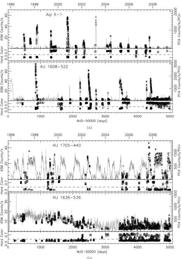
of mass accretion ( ˙M ) from the companion to the compact object can be transient or persistent. A significant amount of gravitational energy is transformed into thermal energy as the mass from the companion spirals through the accretion disk toward the compact object. Observations show that the inner disk reached temperatures & 1 keV, and most of the photons are released in X-rays. A more quantitative description of this scenario is given in Chapter 3. X-ray astronomy started with the discovery of the X-ray binary Sco X–1 in 1960s [Giacconi et al., 1962]. Since then, more than 200 X-ray binaries have been discovered [Guse˘inov et al., 2000]. Our understanding of these sources have been significantly improved in the past decade by the launch of X-ray telescopes with unprecedented capabilities, such as the Rossi X-ray Timing Explorer (RXTE ), BeppoSAX, the Chandra X-ray observatory, XMM-Newton, and Suzaku. I refer to Shapiro and Teukolsky [1983], Lewin et al. [1997], Frank et al. [2002], Lewin and van der Klis [2006] for basic concepts and reviews of X-ray binaries. Figure 1-2 shows some sample X-ray long-term light curves from ASM onboard RXTE . They are from seven NS X-ray binaries, which will be studied in detail in this thesis.

Optical studies of X-ray binaries can reveal the physical properties of the companion [Charles and Coe, 2006]. The mass of the companion is one of the most important factors determining the properties of X-ray binaries. If the mass of the companion is massive (& 10M⊙), the X-ray binaries are called high-mass X-ray binaries (HMXBs). Otherwise, if

the mass of the companion is . 2M⊙, they are called low-mass X-ray binaries (LMXBs).

Because the companion is small, the two stars in LMXBs must be close to each other in order to transfer substantial mass from the NS or BH to the companion. The mass

Figure 1-2: The X-ray long-term light curves of seven NS X-ray binaries observed by RXTE/ASM. These sources will be studied in detail in this thesis.

transfer in LMXBs is normally through the inner Lagrangian point as the companion fills its Roche lobe (Figure 1-1). HMXBs, which mostly have giant or supergiant O and B stars as the companions, can also transfer mass via filling their Roche lobes. However, most HMXBs transfer mass via a vigorous stellar wind, in which case the separation between the companion and the compact object can be large.

The lifetimes of HMXBs are short, ∼ 105 − 107 yr, as they are determined by the evolution timescales of the high-mass companions. On the other hand, the lifetimes of LMXBs are longer, ∼ 107 − 109 yr, and they are determined by the mass-transfer process governed by binary evolution [Tauris and van den Heuvel, 2006]. Thus, HMXBs are found mostly near the Galactic plane, where young massive stars lie, while LMXBs are found mostly towards the Galactic center and in globular clusters. It is believed that a HMXB is formed as the massive companion survived the supernova explosion of its primary, while a LMXB is probably formed via gravitational capture of a NS or BH in the places with high number density of stars, such as the Galactic center and globular clusters. The NS in LMXBs can also be formed by the accretion-induced collapse of a WD. The NS in HMXBs mostly appears as an accretion-powered pulsar, while most NS LMXBs show weak or absence of periodic pulsations.

1.2

Physics in X-ray binaries: why we study them

X-ray binaries provide important cosmic settings for us to study accretion physics. The characteristics of emission from X-ray binaries, from radio to X-ray, or even gamma ray photon energies, vary with the mass accretion rate ( ˙M ), and depend on many physical parameters, especially the nature of the compact object (NS or BH), its mass, the magnetic fields, and the spin of the compact object. We are still developing our understanding of accretion physics, and there are a wide variety of interesting accretion phenomena, such as jets and quasi-periodic X-ray oscillations with limited understanding as to how they depend on the physical parameters.

X-ray binaries also provide unique opportunities to probe the effects of general relativity and the properties of dense matter. The general relativistic effects around the NS and BH are many orders of magnitude stronger than those probed by other tests of general relativity [Psaltis, 2004]. The interior of the NS is denser than atomic nuclei and occupies an environment distinct from both the early Universe and current terrestrial experiments [Hands, 2001].

Here, I briefly introduce one area at the cutting edge of studies of X-ray binaries, i.e., the measurement of BH spin parameters a∗ [Remillard and McClintock, 2006], in order to

show the progress that we have made thus far in study of X-ray binaries. There are several ways that have been used to measure the BH spin parameters, especially the continuum spectral fitting and Fe K line profile. The main idea for the method of continuum spectral fitting is that the spectral fitting can give the information of the radius Rin of the inner

edge of the accretion disk, which can be assumed to be the innermost stable orbit RISCO

predicted by general relativity. RISCO depends only on the BH mass and spin a∗ [Zhang

et al., 1997, Gierli´nski et al., 2001]. Therefore, the estimated size of the inner accretion disk can constrain the BH spin if the mass is known from binary dynamics. The spectra used in such studies are normally taken from the thermal state, where the disk emission in the form of radiated heat dominates the spectra. The assumption of Rin to be RISCO is based

Figure 1-3: The sample CDs (upper panels) and HIDs (lower panels) of NS X-ray binaries. The panels for the columns from the left to the right correspond to the atoll source 4U 1705–44, the “GX” atoll source GX 9+1, the Sco-like Z source GX 17+2, and the Cyg-like Z source GX 340+0, respectively. The data are all from RXTE/PCA. The data of atoll sources span more than ten years, and exposure for each data point is up to 4 ks. Data of GX 17+2 are from 1999 October 3–12, and those of GX 340+0 are from 2001 January 11– 15, with exposure for each data point 128 s. The annotations HS, TS, and SS refer to the hard, transitional, and soft states of atoll sources, respectively, while the annotations HB, NB, and FB refer to the horizontal, normal, and flaring branches of Z sources respectively. See §1.5 for more information.

some range of luminosity, which is believed to be the signature of RISCO. Such a technique

requires many system parameters such as the orbital inclination, distance and BH mass to be well known and involved considerations of many effects such as general relativity and spectral hardening. The Galactic LMXB GRS 1915+105 is measured to have spin parameter a∗ > 0.98 [McClintock et al., 2006].

The BH spin measurement based on Fe K line profile comes from the consideration that the relativistic beaming and gravitational redshift can serve to distort the emission line profile [Miller, 2007]. The extent of this distortion depends on the inner disk radius Rin,

and the fitting of Fe K line can constrain the value of Rin. By assuming Rinto be RISCO, a∗

can be obtained if the BH mass is known, as above. The Fe line emission is believed to be the response of an accretion disk to irradiation by an external source of hard X-rays, which is sometimes seen in the spectra of X-ray binaries. The spin of XTE J1650-500 is suggested to be nearly the maximum using this technique [Miller et al., 2002, Miniutti et al., 2004].

Figure 1-4: The sample unfolded energy spectra (left panels) and power density spectra (right panels) of the BH X-ray binary GRO J1655–40 in different X-ray spectral states. The energy spectra are fit with a multi-color disk (red dotted line), a simple power-law or a cutoff power-law (green dot-dashed line), and a Gaussian Fe line (cyan double-dot-dashed line). The total model fit is shown as a black solid line. Both the energy and power density spectra have been rebinned to improve the signal to noise ratio. The data for top to bottom panels are from observations of RXTE on 1997 August 14, 1997 March 24, 1996 August 29, respectively.

Figure 1-5: The same as Figure 1-4, but for the atoll source 4U 1636–536. Compared with the BH cases, the energy spectral models also include a single-temperature blackbody (blue dashed line). The data for upper and lower panels are from observations of RXTE on 2006 March 22 and 2001 April 30, respectively.

Figure 1-6: The same as Figure 1-5, but for the millisecond and slow accretion-powered X-ray pulsars SAX J1808.4–3658 (upper panels; 2002 October 18) and V 0332+53 (low panels; 2005 February 13). The energy spectrum from V 0332+53 is fitted with a cutoff power-law with the cyclotron resonant lines modeled by three Gaussian absorption lines. Only the total model plus the Gaussian Fe line is shown for this source.

Figure 1-7: The same as Figure 1-5, but for the Z source GX 17+2. The data for top to bottom panels are from observations of RXTE on 1999 October 5, 1998 August 7, 1999 October 11, respectively.

1.3

Techniques used to study X-ray binaries

The information of X-ray binaries is gained from studies of the photons that they emit. The wavelength coverage extends both from radio to X-rays, and to gamma rays. The spectral and timing properties are utilized to understand the source spectral evolution and to reveal the physical parameters. I describe below the techniques that are normally used in the X-ray band. Currently we cannot resolve the LMXBs using direct imaging techniques in X-rays. Thus the techniques used to study them naturally fall into two categories, spectral and timing studies.

The spectral studies include both photometric analyses and spectral fitting methods. In the photometric analyses, X-ray colors are used. An X-ray color is a hardness ratio between the photon counts in two different energy bands and is a rough measure for spectral slope. Two X-ray colors are normally used, i.e., soft and hard colors. They correspond to lower and higher ranges, respectively, where the energy bands are defined. For example, in this thesis, the soft color is defined as the ratio of the counts in the (3.6–5.0)/(2.2–3.6) keV bands, and the hard color is the ratio in the (8.6–18.0)/(5.0–8.6) keV bands. By defining these two colors over appropriate timescales, we can track X-ray spectral variations. The conventional practice is to show a color-color diagram (CD), with the hard color vs. the soft color, and a hardness-intensity diagram (HID), with one color vs. the intensity, i.e., the sum of the count rates in the four bands. Different source types normally display different patterns in the CD or HID. Their patterns normally correspond to several source states or branches. Some examples of CD/HIDs for different types of sources are presented shown in Figure 1-3, using the above definition of colors. I note that the CD/HID is typically combined with timing properties (e.g., power density spectra; see below) so that the source states/branches can be distinguished more effectively.

The spectral fitting method is used in order to obtain more physically meaningful inter-pretations of the X-ray spectra and evolution. Spectra can be accumulated based on time bins (time-resolved spectra) or their positions in the CD/HID (color-resolved spectra). In either way, a single spectrum is intended to characterize a particular condition. Then the spectra are fit against physical models to obtain the physical parameters. This is often car-ried out using the X-ray spectral fitting package XSPEC, which is distributed by NASA and includes many theoretical models [Arnaud, 1996]. Compared with the photometric method, the spectral fitting method heavily depends on the models used, and in some cases, different models lead to very different results, which is called model degeneracy (see, e.g., Chapter 4).

The left panels of Figures 1-4–1-7 show the sample spectral fit of the energy spectra from different classes of ray binaries in different spectral states/branches. It can be seen that X-ray binaries typically show a composite spectrum, i.e., several spectral components needed to explain the whole spectrum. The continuum spectral components for X-ray binaries can be broadly grouped into two classes, i.e., thermal and non-thermal. In this thesis, the thermal components specifically refer to a single temperature blackbody (BB), or a composite of multicolor blackbody such as a multicolor disk (MCD). Non-thermal components typically have a wide energy range, extending into hard X-rays and have a flatter spectral energy distribution than thermal components. The most common non-thermal component seen in X-ray binaries is Comptonization emission. In this thesis, Comptonization refers to the inverse Compton scattering, i.e., photon energies are boosted due to interaction of photons with energetic electrons. More detailed description of X-ray emission mechanisms is presented in Chapter 3.

Timing studies provide information on the properties of rapid variabilities. X-ray emis-sion from X-ray binaries is stochastic process, and the mathematical tool used mostly is Fourier analysis. The Fourier power spectrum of the X-ray count time series measures that variance as a function of Fourier frequency ν in terms of the power density Pν(ν). Several

broad features are normally seen in a typical power density spectrum, and they are believed to correspond to different types of noises. There are sometimes components in the power density spectrum which show discrete peaks. When such features are resolved and thought to arise from non-coherent processes, they are called quasi-periodic oscillations (QPOs). For X-ray pulsars (coherent modulations with some smearing in frequency due to the bi-nary motion or spin changes), the peak at their spin frequency can be extremely sharp, sometimes with width ≪1 Hz. The right panels of Figures 1-4–1-7 show the sample power density spectra from different classes of X-ray binaries in different spectral states/branches. The timing study involves investigation of how different power density spectral components vary as source spectra evolve, with the goal to understand their origins.

1.4

BH and NS X-ray binaries

Based on the nature of the compact object, X-ray binaries are classified into NS and BH types. So far, we cannot obtain direct evidence of the event horizon to prove the existence of BHs. Thus, the classifications of NS and BH X-ray binaries are mostly based on empirical methods attached to theoretical arguments. The strongest evidence for BHs is currently considered to be the measurement of a gravitational mass for a compact object larger than the upper limit in mass for a NS. The upper bound of the NS mass is ∼3 M⊙ [Rhoades

and Ruffini, 1974]. This approach is carried out by measuring the binary mass function, f ≡ PorbK23/2πG = M sin3i/(1 + q)2, where Porb is the orbital period, K2 is the

half-amplitude of the velocity curve of the companion, M is the mass of the compact object, i is the orbital inclination angle, and q is the ratio of the masses of the companion to the compact object. The mass function gives the lower limit of the mass of the compact object, through optical observations of velocity curves of the companions.

The classification of a compact object in the X-ray binary into a NS is warranted if coherent pulsations or type I X-ray bursts are detected. The coherent pulsations, which are at the spin frequency of the NS, is believed to be due to the channeling of accreting material along magnetic field line onto the magnetic poles that are misaligned with the NS rotation axis. The focusing of accretion at the magnetic poles produces hot spots, which rotate in and out of view and cause pulsations. BHs cannot produce a magnetic field to channel the accreting material. There are also no hot spots because a solid surface is required to make them. Type I X-ray bursts (or superbursts) are another signature of a NS, because they are believed represent violent nuclear burning as the accreting material is compressed and heated. Again this requires a solid surface to store the accreted H and He until detonation occurs. The differences in spectral/timing properties are also invoked to distinguish NS and BH X-ray binaries [e.g., Done and Gierli´nski, 2003, Sunyaev and Revnivtsev, 2000]. However, on the whole remarkable spectral and timing similarities exist between NSs and BHs, especially in low luminosity states (see Figures 1-4–1-5).

The BH X-ray binaries are mostly LMXBs, but several of them are known to be HMXBs [McClintock and Remillard, 2006]. Their continuum energy spectra mostly exhibit a com-posite shape consisting of a thermal and a nonthermal component. The thermal component is well modeled by a multi-color disk, while the nonthermal component is usually modeled

by a power-law model (Figure 1-4). There are three dominant active emission states for BH X-ray binaries: thermal, hard, and steep power-law [Remillard and McClintock, 2006]. Roughly speaking, the hard state is dominated by the power-law component with initial photon index around 1.7, while the thermal state is dominated by the thermal disk emission. The important characteristics of the steep power-law state are that the initial photon index of the power-law component is around 2.5 (much higher than that in the hard state), and that there are often strong QPOs (Figure 1-4).

The NS X-ray binaries can be classified based on whether they pulse or show type I X-ray bursts. Coherent pulsations are observational manifestation of strong magnetic field in the compact object. The classical accretion-powered pulsars are those with spin periods of the order of one second or more, and they are called slow accretion-powered pulsars (compared with millisecond pulsars). They are commonly seen in HMXBs, and this is because HMXBs are young systems and their magnetic fields are not expected to evolve away from its high birth value due to accretion. LMXBs mostly are old systems, and their prolonged phase of accretion is thought to have suppressed the magnetic fields of the NS [Psaltis, 2004]. One sample of energy and power density spectra of the slow accretion-powered X-ray pulsar V 0332+53 (with spin period 4.375 s) is shown in the lower panels in Figure 1-6. Clear cyclotron absorption lines are seen. The millisecond accretion-powered X-ray pulsars are one special class of LMXBs that have magnetic field strong enough to produce coherent pulsations at their fast spin frequencies (v > 100 Hz). It should be noted that whether the magnetic field is strong enough to produce coherent pulsations depends the accretion rate too. In the millisecond accretion-powered pulsars, the magnetic field is about 108 _{G, much}

lower than 1012 G often seen in slow accretion-powered pulsars, but their accretion rates are low on the whole too, among the lowest in the known LMXB population. The energy spectra of millisecond accretion-powered pulsars are mostly hard (Figure 1-6).

The weakly magnetized accreting NSs are mostly found in LMXBs. They can be clas-sified into Z and atoll sources [Hasinger and van der Klis, 1989]. They will be focus of this thesis. Thus their properties will be presented in the next section in more detail. Weakly magnetized accreting NSs normally show type I X-ray bursts, but generally no strong co-herent pulsations, except the millisecond accretion-powered pulsars.

1.5

Weakly magnetized NS LMXBs

Z and atoll sources are the two main classes of weakly magnetized NS LMXBs. They are classified based on their X-ray spectral and timing properties [Hasinger and van der Klis, 1989, van der Klis, 2006]. They were named after the patterns that they trace out in the CDs or HIDs [Hasinger and van der Klis, 1989]. Figure 1-3 shows the CD/HIDs of two atoll sources (first two columns) and two Z sources (last two columns). It should be noted that atoll sources originally were thought to have only atoll patterns in the CD/HIDs, but with extensive coverage by RXTE , some atoll sources can have Z-like patterns [Muno et al., 2002, Gierli´nski and Done, 2002a], such as those in the first column in Figure 1-3. However, Z and atoll sources are still two distinct classes with differences in many aspects. Their patterns have different orientation, color ranges, evolution timescales. Z sources typically radiate at luminosities close to Eddington luminosity (LEDD), while atoll sources cover a lower and

larger luminosity range (∼0.001–0.5 LEDD). Furthermore, the spectra of Z sources are very

soft on all three branches of the “Z”, whereas the spectra of atoll sources are soft at high luminosities, but hard when they are faint (Figures 1-5 and 1-7). Properties like the rapid

X-ray variability and the order in which the branches are traced out are also different for the two classes [Barret and Olive, 2002, van Straaten et al., 2003, Reig et al., 2004, van der Klis, 2006]. As denoted in Figure 1-3, the upper, diagonal and lower branches of the Z-shaped tracks for Z sources are called horizontal, normal and flaring branches (HB/NB/FB), respectively, while for atoll sources, they are called the hard, transitional and soft states (HS/TS/SS), respectively (or extreme island, island, and banana states, respectively). As will be shown in §5, the differences between Z and atoll sources are due to their different mass accretion rates.

Atoll sources include ordinary atoll sources and “GX” atoll sources. “GX” atoll sources include GX 3+1, GX 9+1, and GX 9+9 (GX 13+1 is sometimes included in this class, but it shows some peculiar behavior) [van der Klis, 2006]. They are all in the galactic bulge and are all persistent, with luminosity believed to be roughly higher than ordinary atoll sources. “GX” atoll sources are only observed in the soft state thus far. Some ordinary atoll sources are persistent (e.g., 4U 1636–53 and 4U 1705–44), while the others are transient (e.g., Aql X–1 and 4U 1608–52; Figure 1-2).

As mentioned above, Z sources have three distinct branches. Based on the shape and orientation of their branches, the six classical Z sources were further divided into two sub-classes [Kuulkers et al., 1994]: Cyg-like (Cyg X-2, GX 340+0, and GX 5-1) and Sco-like (Sco X-1, GX 17+2, and GX 349+2; Figure 1-3). In addition to movement along the “Z” tracks, the Z tracks themselves display slow shifts and shape changes in CDs/HIDs. These so-called secular changes are most apparent in Cyg X-2. XTE J1701–462 is a new transient accreting NS X-ray binary, with a long outburst in 2006–2007 (Figure 1-2). It exhibited both Z source and atoll source behavior.

One of the most important tasks of understanding accreting NSs is to reveal the origin of their spectral evolution. This includes not only the origin of different states/branches, but also the origin of secular changes of Z source tracks and transformation of source types. To achieve this, we need to have a correct spectral model for these systems. However, the spectral modeling of accreting NSs has been controversial for a long time [see Barret, 2001, for a review].

1.6

Organization and content of thesis

The main focus of this thesis is on the spectral evolution of weakly magnetized accreting NS X-ray binaries. They include both Z and atoll sources. This investigation considers the spectral decomposition problem of these systems, the physical origin of spectral evolution, and the transformation from one source type to the other.

Chapter 2 introduces the X-ray observatories RXTE , Suzaku, and BeppoSAX, and their data analysis methods. They will be used extensively in this thesis.

Chapter 3 describes in more detail some fundamental accretion physics and the X-ray emission mechanisms relevant to X-ray binaries.

Chapter 4 is a published paper on the spectral modeling for atoll sources, concentrating on two transients Aql X–1 and 4U 1608–52. I compare different models that have been used for these systems and come up with a new way to model the spectra of these systems. The new model is shown to describe the spectral evolution of atoll sources better in terms of some desirability criteria, including LX ∝ T4 evolution for the multicolor disk (MCD)

component, and the similarity to black holes (BHs) for correlated timing/spectral behavior. Chapter 5 examines our new spectral model (Chapter 4) to the highly variable atoll

source 4U 1705–44 using the extended soft X-ray sensitivities of Suzaku and BeppoSAX. Chapter 6 applies our new spectral model on two persistent atoll sources 4U 1636–536 and 4U 1705–44. In this paper, I examine the soft state more carefully by comparing the results from the part of the soft state with kHz QPOs detected with those from other parts. Because this difference from Chapter 4, I also include Aql X–1 and 4U 1608–52 in this chapter. The conclusions in this chapter are mostly the same as those in Chapter 4, but I also find a close relation between the kHz QPOs and the accretion disk.

Chapter 7 is a published paper on the spectral evolution of XTE J1701–462. Physical interpretations are given for the 3 branches of Z sources, and I explain the cause of the transformation between Z and atoll types.

In Chapter 8, I present the study of type I X-ray bursts from XTE J1701–462 and estimate the distance to this system.

In Chapter 9, I study the Sco-like Z source GX 17+2 in order to see whether our interpretations of Z tracks of XTE J1701–462 apply to persistent Z sources.

I summarize our study results of NS X-ray binaries and present the complete picture of their spectral evolution and transformation of source types in Chapter 10. The conclusions are presented in Chapter 10.

Chapter 2

X-ray Observatory and Data

Analyses

In this chapter I briefly describe the Rossi X-ray Timing Explorer, Suzaku, and BeppoSAX, which are the X-ray observatories that provide the data used in this thesis. I will describe the relevant data reduction techniques that are common to the detailed studies reported in the later chapters.

2.1

The Rossi X-ray Timing Explorer

The Rossi X-ray Timing Explorer [RXTE , Bradt et al., 1993] is an X-ray mission, which features unprecedented time resolution in combination with moderate spectral resolution to explore the variability of X-ray sources. It was launched on December 30, 1995 from NASA’s Kennedy Space Center by a Delta II rocket into its intended low-earth circular orbit at an altitude of 580 km, corresponding to an orbital period of about 90 minutes, with an inclination of 23◦. A diagram of the RXTE is shown in Figure 2-1, with three major instruments labeled, i.e., the Proportional Counter Array [PCA; Jahoda et al., 1996], the High Energy X-ray Timing Experiment [HEXTE; Rothschild et al., 1998], and the All-Sky Monitor [ASM; Levine et al., 1996]. The PCA and the HEXTE are collimated (non-focusing) pointed instruments, while the ASM is a coded-mask imaging instrument designed to survey the sky with a wide viewing angle. RXTE has been carrying out science observations for more than 12 years, far surpassing its required lifetime of two years.

2.1.1 Instruments

The PCA is an array of five Proportional Counters Units (PCUs) with a large total collecting area of 6500 cm2_{. It can detect sources as faint as 0.1 mCrab. It only carries out pointed}

observations, with the FWHM spatial resolution confined to be 1◦ by the collimator. It is sensitive to energy range 2.5–60 keV with energy resolution < 18% at 6 keV. The PCA has been well calibrated, based on observations of the Crab Nebula. The data can be collected at time resolution of 1 µs. The PCA data, which are processed by the Experiment Data System before telemetered, are collected in a variety of modes corresponding to different combinations of time and energy resolution in order to stay within the mission’s telemetry limit. However, there are two modes, known as ‘standard1’ and ‘standard2’, that are made for every observation. Standard1 data contain 0.125-s full-energy-band light curves for

Figure 2-1: Diagram of the RXTE spacecraft, with major instruments labeled. Figure courtesy of the NASA High Energy Astrophysics Science Archive Research Center/Goddard Space Flight Center (HEASARC/GSFC).

every PCU and for different types of instrument background rates. Standard2 data has a time resolution of 16s and 129 energy channels covering the full energy range of the PCA detectors. Some of the PCUs suffer breakdown and trip off if they are not regularly “rested”. This means that any individual observation may contain data from 1 to 5 operating PCUs. The HEXTE is composed of two clusters (A and B) consisting of four “phoswich” scin-tillation detectors each. These two clusters rock on and off the source along mutually orthogonal directions for realtime background measurements. Cluster A started experienc-ing rockexperienc-ing problems in 2006, and since then it was fixed in the on-source position. The detectors are sensitive to high-energy X-rays from 15-250 keV. The energy resolution is 15% at 60 keV. The FWHM spatial resolution for the HEXTE is also 1◦. Each cluster has collecting area of 800 cm2. The time resolution can be as high as 8 µs. The HEXTE has one standard mode that is used for every observation. This mode has 16-s time resolution and 64 spectral channels.

The ASM consists of three wide-angle shadow cameras equipped with proportional coun-ters with a total collecting area of 90 cm2. It scans about 80% of the sky every 90 minutes, with additional gaps if the satellite orbit crosses through the South Atlantic Anomaly. It can monitor sources of 30 mCrab or brighter, and have spatial resolution of 3′ _{× 5}′_{. The}

ASM standard products consist of light curves and color measurements for each of the ∼566 sources (at the present time) in the ASM catalogue.

2.1.2 Data Analyses

The studies of X-ray binaries rely on their spectral and timing information and involve creation of light curves, energy spectra, color diagrams, and power density spectra, etc., on appropriate timescales. The data analyses typically start with filtering of the data for proper observing conditions, accumulate data over energy/time bins, and transform in ways depending the types of data products, and finally compare/fit them with spectral/timing models as needed. Most observatories, including RXTE , Suzaku and BeppoSAX, provide main data products in the FITS (Flexible Image Transport System) format. They can be analyzed using the FTOOLS software package, which is part of the HEAsoft provided by NASA’s High Energy Astrophysics Science Archive Research Center (HEASARC). FTOOLS provides general and mission-specific tools to manipulate FITS files. In the following I describe the procedures used in most part of this thesis to reduce data from RXTE . I will start with the PCA first.

Some standard criteria were used to filter the PCA data: the earth-limb elevation angle was required to be larger than 10◦_{, and the spacecraft pointing offset was required to be}

< 0.02◦. For faint observations, we additionally excluded data within 30 minutes of the peak of South Atlantic Anomaly passage or times with large trapped electron contamination. In most part of this thesis, the focus is on spectral evolution, and only the persistent emission due to gravitational accretion is relevant. Emission due to stable nuclear burning might present, but is negligible compared with the persistent emission due to gravitational accretion (Chapter 3). Sometimes, however, the source emission can be dominated by unstable nuclear burning leading to type I X-ray bursts, which occurs over very short intervals (a few seconds to minutes). Such intervals should be excluded. In this thesis, I exclude data of 20 seconds before and 200 seconds after type I X-ray bursts [see Remillard et al., 2006a].

To create PCA spectra, “standard 2” data were normally used. As the PCA is a colli-mated instrument and is always pointed at the source during an observation, the background

is not directly available, but is estimated by models, which are provided by the PCA team. As suggested by the PCA team, I used appropriate faint/bright background models when the source had intensity lower or higher than 40 counts/s/PCU, respectively. The integra-tion time for each spectrum depends on source variability. It can be one spectrum for each observation, or one spectrum for several observations, or several spectra for one observation. When necessary, the integration time can be selected based on positions in the CD/HIDs. In order to carry out spectral fitting and because of PCA response varying with time, I create and select response files appropriate to the time of each spectrum that is analyzed.

The hard/soft colors used in the CD/HIDs are based on PCA spectra. Soft and hard colors were defined as the ratios of the background-subtracted counts in the (3.6–5.0)/(2.2– 3.6) keV bands and the (8.6–18.0)/(5.0–8.6) keV bands, respectively [Muno et al., 2002]. We normalized the raw count rates from each PCU with the help of observations of the Crab Nebula. For each PCA gain epoch, we computed linear fits (vs. time) to normalize the Crab count rates to target values of 550, 550, 850, and 570 counts/s/PCU in these four energy bands. The CD/HIDs using PCA data presented in this thesis are all normalized in this way.

In timing analyses, the common mathematical tool is the power density spectra calcu-lated through discrete Fourier transform. PCA data instead of HEXTE data are normally used for timing analyses, since accreting NSs emit photons most intensely at energies below 20 keV. Data with high time resolutions are necessary in order to probe rapid variability. Thus binned or event mode data, instead of standard mode data, are used for this purpose. Detailed calculation of power density spectra is presented in the Appendix A. They are normally Leahy-normalized and have Poisson noise subtracted. The deadtime correction is also necessary for sources with high intensity. The resulting power density spectra can be fit with model consisting of different noise components and QPOs. The power continuum can be integrated over some frequency range (0.1-10 Hz in this thesis) to obtain the fractional root-mean-square values, to characterize source variability in that frequency range.

In this thesis, the HEXTE data are only used to create spectra that have integration time matching that of PCA spectra. The background spectra can be directly made from off-source observation data. Most of observations of Cluster A after 2006 only have on-source observation data due to rocking problems, and the background should be estimated using the hextebackest tool. It is based on the off-source observations of Cluster B. The deadtime correction for HEXTE data is made using the program provided by the HEXTE team. The response file for each cluster of the HEXTE has been the same throughout the RXTE mission and is provided directly by the HEXTE team.

2.2

Suzaku

Suzaku[Mitsuda et al., 2007] is Japan’s fifth X-ray astronomy mission and was launched in August 2005. The goal of this mission is to carry out high resolution spectroscopy and wide-band observations of high energy astronomical phenomena. It covers the energy range 0.2– 600 keV with the two instruments, i.e., X-ray CCDs [X-ray Imaging Spectrometer; XIS;0.2– 12 keV Koyama et al., 2007], and the hard X-ray detector [HXD; 10–600 keV Takahashi et al., 2007]. Suzaku also carries a third instrument, an X-ray micro-calorimeter (X-ray Spectrometer; XRS), but the XRS lost all its cryogen before routine scientific observations could begin. The XISs and HXD are imaging and collimated instruments respectively. Broadband spectral feature and high energy resolution of this X-ray observatory make it

Figure 2-2: Diagram of the Suzaku spacecraft, with major instruments labeled [Mitsuda et al., 2007].

highly suitable for X-ray binary studies.

2.2.1 Instruments

XISs

The Suzaku X-ray CCD instrument consists of four XIS cameras. They employ X-ray sensitive silicon charge-coupled devices (CCDs), which are operated in a photon-counting mode. In general, X-ray CCDs operate by converting an incident X-ray photon into a charge cloud, with the magnitude of charge proportional to the energy of the absorbed X-ray. This charge is then shifted out onto the gate of an output transistor via an application of time-varying electrical potential. This results in a voltage level (often referred to as “pulse height”) proportional to the energy of the X-ray photon.

The four Suzaku XISs are named XIS0, 1, 2 and 3, each located in the focal plane of an X-ray Telescope. XIS2 has not been used for scientific observations since November 2006, due to a large amount of charge leakage. XIS1 uses a back-illuminated CCDs, while the other three use front-illuminated CCDs. The CCD performance gradually degrades in space due to the radiation damage. This is because of the accumulation of charge traps that are produced by cosmic-rays. One of the important features of the XIS is the capability to inject small amounts of charge to the pixels. Periodic charge injection is quite useful to fill the charge traps, and to make them almost harmless. This method is called the spaced-row charge injection (SCI), and the SCI has been adopted as a standard method since AO-2 to cope with the increase of the radiation damage.

There are two different kinds of on-board data processing modes for XISs, i.e., the Clock and Editing modes. The Clock modes describe how the CCD clocks are driven, and this determines the exposure time, exposure region, and time resolution. The Clock modes include normal modes, which is explained in more detail below, and Parallel Sum Mode, in which the pixel data from multiple rows are summed in the Y-direction on the CCD, and the sum is put in the Pixel RAM as a single row. The Editing modes specify how detected events are edited, and this determines the format of the XIS data telemetry. One example of edit modes is the 5 × 5 observation mode, in which all the pulse heights of the 25 pixels centered at the event center are sent to the telemetry. There are also 3 × 3 and 2 × 2 observation modes.

In the Normal Clock mode, the Window and Burst options can be specified, otherwise all the pixels on the CCD are read out every 8 seconds. The Window and Burst options are important when observing bright X-ray binaries, because the pile-up problem can be reduced by faster readout times. Pile-up occurs when more than one photon strikes in the same or adjacent pixels in one CCD readout frame. The Window option allows shorter exposure times by reading out more frequently only a portion of the CCD. The full CCD has 1024×1024 pixels. When the Window width is 256×1024 pixels (1/4 Window), the exposure time becomes a quarter of that without the Window option (i.e., 2 s), and the Pixel RAM is filled with the data from four successive exposures. Similarly, there can be 1/8 or 1/32 Window options. In the Burst option, an extra deadtime t is introduced for every exposure. If the pixel is read out, say, every 2 s for 1/4 Window, the live time is 2-t s in every exposure. The Burst and Window options are independent and may be used simultaneously. They can effectively reduce the pile-up problem. For example, the XIS team expects that a point source as bright as 12.5 counts/s/XIS can be observed with the pile-up problem being negligible if neither options are specified. Then if the 1/N Window

option and deadtime of t s for the Burst option are specified, a point source as bright as 12.5×N × 8/(8 − Nt) counts/s/XIS can be observed with the pile-up problem being negligible.

HXD

The HXD is a hard X-ray scintillating instrument, and has a main purpose to extend the bandpass of the Suzaku observatory to the highest feasible energies, thus allowing broad-band studies of celestial objects. The HXD sensor is a compound-eye instrument, consisting of 16 main detectors. Each unit actually consists of two types of detectors: a GSO/BGO phoswich counter, and 2mm-thick PIN silicon diodes located inside the well, but in front of the GSO scintillator. The PIN diodes are mainly sensitive below ∼ 60 keV, while the GSO/BGO phoswich counter (scintillator) is sensitive above ∼ 40keV. The HXD features an effective area of ∼ 160 cm2 _{at 20 keV, and ∼ 260 cm}2 _{at 100 keV. The energy resolution}

is ∼ 4.0 keV (FWHM) for the PIN diodes, and 7.6/√E% (FWHM) for the scintillators, where E is energy in MeV. The HXD time resolution is 61 µs.

2.2.2 Data Analyses

The extraction of light curves or spectra of XISs can be done within the program xselect provided by FTOOLS. As this thesis deals with X-ray binaries and they can be treated as point sources, one spatial region on the CCD measures the source, while a different other region away from the source position can be used to measure the background. A radius of 250 pixels (260′′_{) of the circular source extraction region can ensure that 99% of}

the flux of a point source is included. For bright sources, the background region can be significant contaminated by source emission, but in this case, background subtraction might be unnecessary, as the source is so much brighter than the background. As the response of XISs varies with time, response files close in time to each spectrum must be created, and we used the xisrmfgen and xissimarfgen provided by the XIS team to accomplish this task.

When the sources are bright, the XIS CCDs can still experience serious event pile-up, even when the Window and Burst options are used. Normally, the center region with serious pile-up should be excluded. In this thesis, I estimated the pile-up fraction of each CCD pixel using two publicly available tools aeattcor.sl and pileup_estimate.sl. Their results were used to exclude regions with the local pile-up fraction > 5%. For more information of both tools, we refer to the website http://space.mit.edu/CXC/software/suzaku/.

The extraction of light curves or spectra for the HXD/PIN and the HXD/GSO can also be carried out in xselect program in FTOOLS. The procedures are very similar between the PIN and GSO, and I here describe them for the HXD/PIN only. As it is a collimated instrument, no spatial extraction region needs to be specified. The background includes two parts, i.e., the cosmic X-ray background and the non X-ray background. The non X-ray background is distributed to users as simulated event files tailored to each observation. The cosmic X-ray background can be simulated based on the typical cosmic X-ray background model using XSPEC. The response files for the HXD/PIN are provided by the HXD team for different instrument setting epochs.

Figure 2-3: Diagram of the BeppoSAX spacecraft, with major instruments labeled [Boella et al., 1997a].

2.3

BeppoSAX

BeppoSAXwas a past X-ray mission which operated from 1996 April 30 till 2002 April 30. It was a program of the Italian Space agency with participation of the Netherlands Agency for Aerospace programs. One of its important goals was to make broad band spectroscopy of different classes of X-ray sources, with the energy coverage 0.1–300 keV. It carried four narrow field instruments (Figure 2-3): the Low Energy Concentrator Spectrometer [0.1–10 keV, LECS; Parmar et al., 1997], the Medium Energy Concentrator Spectrometer [1.3–10 keV, MECS; Boella et al., 1997b], the High Pressure Proportional Gas Scintillation Counter [8–50 keV, HPGSPC; Manzo et al., 1997], and the Phoswich Detection System [15–300 keV, PDS; Frontera et al., 1997]. The LECS and MECS are imaging instruments, while the HPGSPC and PDS are collimated instruments. The HPGSPC had operation problems and has no data publicly available. Thus below I only focus on the other three instruments. BeppoSAXalso carried two coded mask proportional counters (Wide Field Cameras, WFC; Figure 2-3), that provide access to large regions of the sky in the range 2–30 keV. Each WFC has a field of view of 20◦ _{× 20}◦ (FWHM) with a resolution of 5′. In this thesis, the WFC is not used and thus is not described in detail.

2.3.1 Instruments

LECS and MECS

The MECS is a set of three identical grazing incidence telescopes with a double-cone geom-etry. The detectors were position sensitive gas scintillation proportional counters in their focal planes. Three units are named as MECS1, 2, 3. They have total effective area 150 cm2 at 6 keV, FOV 56′ _{in diameter, angular resolution 1.2}′ _{at 6 keV, and energy resolution}

depending on energy E as 8 × (E/6keV)−0.5_{% (FWHM). MECS1 did not operate for very}