Snow creep pressures: effects of structure boundary conditions and snowpack properties compared with field data

(1)

Publisher’s version / Version de l'éditeur:

Cold Regions Science and Technology, 17, September 1, pp. 33-47, 1989-09-01

READ THESE TERMS AND CONDITIONS CAREFULLY BEFORE USING THIS WEBSITE. https://nrc-publications.canada.ca/eng/copyright

Vous avez des questions? Nous pouvons vous aider. Pour communiquer directement avec un auteur, consultez la première page de la revue dans laquelle son article a été publié afin de trouver ses coordonnées. Si vous n’arrivez pas à les repérer, communiquez avec nous à PublicationsArchive-ArchivesPublications@nrc-cnrc.gc.ca.

Questions? Contact the NRC Publications Archive team at

PublicationsArchive-ArchivesPublications@nrc-cnrc.gc.ca. If you wish to email the authors directly, please see the first page of the publication for their contact information.

NRC Publications Archive

Archives des publications du CNRC

This publication could be one of several versions: author’s original, accepted manuscript or the publisher’s version. / La version de cette publication peut être l’une des suivantes : la version prépublication de l’auteur, la version acceptée du manuscrit ou la version de l’éditeur.

Access and use of this website and the material on it are subject to the Terms and Conditions set forth at

Snow creep pressures: effects of structure boundary conditions and

snowpack properties compared with field data

McClung, D. M.; Larsen, J. O.

https://publications-cnrc.canada.ca/fra/droits

L’accès à ce site Web et l’utilisation de son contenu sont assujettis aux conditions présentées dans le site LISEZ CES CONDITIONS ATTENTIVEMENT AVANT D’UTILISER CE SITE WEB.

NRC Publications Record / Notice d'Archives des publications de CNRC:

https://nrc-publications.canada.ca/eng/view/object/?id=a7740d89-c555-481c-aa1b-641d37cd0cb7 https://publications-cnrc.canada.ca/fra/voir/objet/?id=a7740d89-c555-481c-aa1b-641d37cd0cb7

(2)

Ser

National Research Consell national

T H ~

I

Councii Can*

mc,wctm can*

N 2 1 d

no

.

1 6 2 2 institute for

-

Institut de

c. 2 Research in recherche en

BLDG

Construction construction

Snow Creep Pressures: Effects of Structure

Boundary Conditions and Snowpack

Properties Compared with Field Data

by D.M. McClung and J.O. Larsen

Reprinted from

Cold Regions Science and Technology Vol. 17, 1989 p. 33-47

(IRC Paper No. 1622)

NRCC 30953 N 8 C

-

CISTI

L I B R A R Y

I

I R C

CN?C

-

lClST

I.

(3)

l'intemption &s

C161lltnts

de

#formation

du manteau nival dans le sens

de

la pente. Les

prtssions

de

fluage qui

en dsultent constituent souvent le principal factew

B

prendre en

compte

dans

la

conception.

Les

auteurs

de

ce

document fournissent des dondes de

terrain

(pssions) pntcrses

et font

une maly

slc

thCorique du probl&me

B

l'aide d'une loi du fluage

lintairc

visant

dtfvlir

la deformation de la neige. 11s formulent des expressions

analytiques repdsentant les pressions et monaent

que

la t h h b

lidaire

dsultante sous-

estime d'environ 20

%

les pressions moyennes.. Pour en arriver

B

une plus grande

(4)

Cold Regions Science and Technology, 17 ( 1 9 8 9 ) 33-47

Elsevier Science Publishers B.V., Amsterdam - Printed in The Netherlands

SNOW CREEP PRESSURES: EFFECTS OF STRUCTURE BOUNDARY CONDITIONS

AND SNOWPACK PROPERTIES COMPARED WITH FIELD DATA

D.M. McClung and J.O. Larsen

Institute for Research in Construction, National Research Council of Canada, 3 6 5 0 Wesbrook Mall, Vancouver, B. C. V6S 2L2 (Canada)

Norwegian Geotechnical Institute, Postboks 4 0 Taasen, N-080 1 Oslo 8 (Norway) (Received September 29, 1988; revised and accepted February 15, 1989)

ABSTRACT

Structures placed in deep snowcovers are subject to forces caused by the interruption of the downslope snowpack deformation components. The resulting creep pressures are often the primary design consid- eration. In this paper, accurate field data (pressures) and theoretical analysis of the problem using a lin- ear creep law to define snow deformation are pre- sented. Analytical expressions for the pressures are presented and it is demonstrated that the resulting linear theory underestimates the mean pressures by about 20%. Higher accuracy will require a non-lin- ear deformation law.

INTRODUCTION

When structures are erected in deep snowcovers, snow creep pressures are often the primary design consideration. Important examples include: avalanche defences in starting zones, ski lift and pow- erline towers. Although it is relatively easy to build structures which can withstand creep pressures, the cost penalty for structures which are much stronger than necessary is often prohibitive. High accuracy is also required because anchoring conditions in mountainous terrain are often very poor; even if a structure is built to withstand creep loads, expected creep pressures can dictate the position of structures. Conversely, it can be very expensive and po-

I

tentially dangerous if structures standing in deep

snowcovers fail. These considerations underline the

importance of accuracy in specification of creep loads for both cost and safety.

For a given snowpack, two elements control the distribution and magnitude of forces on structures: ( a ) the boundary conditions on the face of the structure and at positions where the snowpack contacts the ground; and ( b ) the rheology of the material. In this paper, the effects of boundary conditions are quantified and compared with two sets of field data from a plane-strain configuration. Calcu- lations are given over the range of expected boundary conditions appropriate to available data. In addition, simple depth variations in snowpack density and stiffness are explored using linear rheology. Taken together, the data and calculations show that a complete definition of the design loads will require a non-linear creep deformation law to be for- mulated for alpine snow.

MODELLING CONCEPTS

Alpine snow has a unique combination of physical properties which have not yet been formalized in a non-linear deformation law suitable for engineering applications. The properties include: high porosity, high temperature (relative to its melting point), and very low strength (it is the weakest natural geotechnical material). These properties combine to produce slow deformation which can pro- ceed even without an applied load. The high porosity results in continuous densification throughout the winter through irreversible deformation (chiefly

(5)

from grain rearrangement). This viscous (or plas- tic) deformation may be described as non-steady creep.

Since simple non-linear deformation laws are not available, a linear deformation law is applied in this paper. The linear formulation yields analytical expressions and it provides information on the importance and character of non-linear effects for the plane-strain configuration.

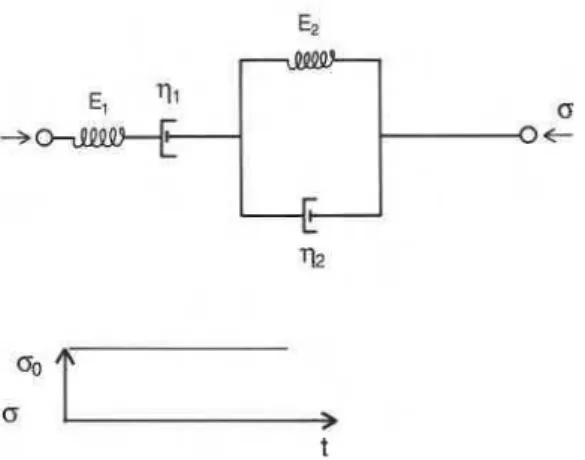
Our approach describes the deformation by gen- eralizing linear visco-elastic behaviour from a one-

dimensional four parameter Burger Fluid (Fig. 1 ).

For a creep test (the load diagram is a Heaviside

function; see Fig. 1 ), the creep compliance relation

may be represented by a proportionality between

strain, e, and load stress, a,:

In Eq. 1, t is time, q,, q2 are viscous moduli and E l ,

E, are elastic moduli. Expression 1 is considered

flexible enough to account for deformation of alpine snow to a first approximation (Bader, 1962;

Mellor, 1975 )

.

For the model, t-tO describes initial elastic re- sponse and as t becomes large relative to to-= q,/E2 the loads are approximated in terms of viscous deformation. For the long time limit, the appropriate

( 3 1

t

Fig. 1 . Schematic of four parameter Burger fluid and Heavi-

side load diagram to represent snow deformation.

state variable, to describe the deformation, is the

strain-rate,

i,

and Eq. 1 reduces to:

when t >> to.

Our model is an engineering formulation for describing the effects of interruption of slow, viscous creep by a rigid structure on a slope with a deep snowcover. Field data (McClung, 1975) show that transient creep rates in new snow layers persist for several days following a storm but these visco-elastic effects are ignored here.

Even if rapid, transient creep rates are not present, the creep loads on a structure will still be time dependent because alpine snow is continuously densifying (making steady state creep impossible). However, the effect is very slow for a deep snowcover which has been present for several months on a slope. For design purposes, the time of interest is late winter or early spring when snow depth is maximum and densification is slow. Therefore, with a linear model it is possible to treat time dependence by exploring variations in the moduli as time pro- ceeds but with constant values at a given instant of time.

Generalization of the one-dimensional model to three dimensions (including both deviatoric and hydrostatic components) is well known. Lang and

Nakamura ( 1984) provide a rigorous treatment.

For long term response, Eq. 2 becomes:

where p, q are shear and bulk viscosity and a,., e,

are stress and strain-rate tensor components in rec-

tangular Cartesian coordinates,

4,

is the sum of the

diagonal components of the strain-rate tensor, and bi, is the Kronecker delta. Equation 3 is equivalent to a linear, compressible Newtonian viscous fluid with neglect of the static pressure term. The static term is unnecessary for describing alpine snow (Salm, 1967) because a state of rest is not possible. Information about values of bulk viscosity is scarce, so it is natural to relate the shear and bulk viscosity by the viscous Poisson's ratio introduced

(6)

SNOW CREEP PRESSURES

Values for v are summarized by Salm ( 1977) and

estimates of p are given by Haefeli ( 1967). This pair

I _{of parameters can be used to describe linear creep}

deformation in general but for plane strain solu-

, tions v will be the only parameter to appear.

Both ,u and q may depend on snow density, tem-

perature, structure and time for a linear theory. For a non-linear formulation they may also be taken to depend on invariants of the stress and strain rate tensor (a case excluded in this paper).

SNOW GLIDING

The boundary conditions at positions where the snowpack is in contact with the ground are crucial for determining structure forces when the ground is smooth and wet. Snow glide (slip of the entire snowpack over sloping ground) can initiate when the interface between the snowpack and the ground is at 0 " C and for slope angles in excess of 1 5 "

.

When vigorous gliding takes place, the highest forces on structures are produced and, therefore, no serious model would exclude this force component.

The fundamental problem of snow gliding is to relate the snowpack drag to the glide velocity. The present theory contains the assumption that glide occurs by creep over the ground roughness elements. When the interface is at O°C, the presence of free water is guaranteed there. This condition implies that the internal velocity field is tangential to the interface when the snowpack contacts roughness elements and that there is no shear stress at those positions. At positions for which the snow- pack is not in contact with the interface (e.g. small roughness elements drowned by water), the drag is

negligible ( McClung and Clarke, 1987 )

.

Assuming

the deformation field is governed by Eq. 3, the tangential snowpack drag, .so, is related to the glide velocity, U, by:

where DA(x,y), the stagnation depth, is a function of the geometry of the interface ( x and y are up and cross-slope directions) and A, the area for which the snowpack is not in contact with the bed. In practice, the stagnation depth must be measured (e.g. Mc-

Clung, 1975 ) or estimated theoretically. If A = 0, Eq.

5 reduces to the theory of McClung (1981 ) for

which a continuous, infinitesimal thin water film was assumed all along the interface. McClung and

Clarke ( 1987 ) provide estimates of D A for A # 0. If

A+m, D*+m and r0+O (an unstable condition). If the interface is sufficiently rough or if it is be-

low O°C, DA=O and U=O. If

v+

4,

corresponding

to incompressibility, Eq. 5 reduces to an analogous expression derived from the same assumptions, but using a linear, incompressible material initially instead of Eq. 3 (e.g. Kamb, 1970).

Pore pressure effects are expected to be small for alpine snow and we will ignore them. Transient (time dependent) effects implied by variations of supply and drainage of basal water are neglected in the theory but their effect on drag reduction is re-

tained when A # 0.

PLANE STRAIN EQUATIONS

In this paper, we wish to compare field data with predictions at the centre of a long retaining wall (avalanche defence structure) perpendicular to the snow-earth interface on a long slope without cur- vature. This configuration is simple enough that one-dimensional solutions are available (McClung, 1982; McClung et al., 1984) to describe the average pressure on the face of the structure using Eqs. 3-5. For a given snowpack, the solutions depend only on

v and D* (or DA) (a mean value all along the inter-

face is defined) and the slope angle y/. The bound-

ary conditions on the face of the stnicture also influence the solutions significantly.

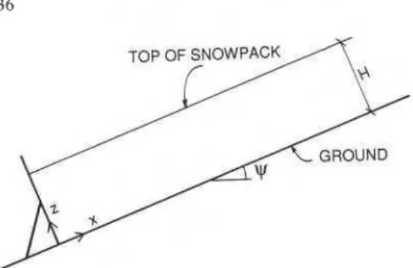
One-dimensional equations (geometry in Fig. 2) are defined by depth averaged quantities (denoted by a bar):

H

where H is snowpack depth measured perpendicu-

lar to the snow-earth interface.

For one-dimensional deformation parallel to the slope, Eq. 3 becomes:

(7)

Fig. 2 . Schematic of plane strain configuration for measuring creep pressures.

where k z duldx is the compressional strain rate, and u is the slope parallel creep velocity component.

Similarly, the equilibrium equation is:

with zg=pgH sin y, p is density, g is acceleration

due to gravity, 7, is snowpack drag at the interface

(due to creep and glide).

With D* and v taken constant throughout the zone of influence of the structure, the solution of Eqs. 5, 7 and 8 at x=O (the structure location; see Mc- Clung, 1982) is of the form:

In Eq. 9, &(O) and the dimensionless parameter L l

H depend on v, y and the boundary conditions on

the structure.

BOUNDARY CONDITIONS ON THE STRUCTURE

The boundary conditions on the face of structures buried in snowcovers are unknown. However, it is possible to place bounds on the possible boundary conditions. Regardless of the conditions on traction or displacement parallel to the structure, the creep velocity perpendicular to the structure may

be taken as u = 0 along the face.

For a rough structure in a cold snowpack, the vertical creep velocity may be approximated as v=O.

The pair of boundary creep velocities (u = v= 0) will

be referred to as the no-slip condition. This condi-

tion is expected from results on snow gliding: glide is not observed on a rough surface unless free water (wet snow) is available. The no-slip condition implies a shear stress along the structure face and causes the maximum force to occur at an angle other than perpendicular to the structure.

At the other extreme, for a smooth structure lu- bricated by free water, a traction free condition,

z,,= 0, along the structure is expected. This pair of

conditions (u = z,, = 0) will be termed the traction-

free condition. For the intermediate case (both slip and traction occur parallel to the structure), a relation analogous to Eq. 5 may be appropriate. This situation is not explored here explicitly; it should produce pressures intermediate between the no-slip and traction-free conditions which bound the problem.

PLANE STRAIN SOLUTIONS

To compare with field data, it is of interest to pre- dict the forces perpendicular and parallel to the structure (shear forces). These are both represented in the maximum principal stress which is the highest force component on the structure.

Traction-free boundary condition

The traction-free boundary condition is the eas- ier of the two extremes to model in one dimension.

In this case T(0) = T,,(O) = O all along the structure

and since u= U= 0 there, the condition is compati-

ble with the glide relation 5. Also, two-dimensional

finite-element solutions show that the normal forces are not appreciably changed from their values without the presence of the wall and therefore the depth- averaged normal stress is approximately:

@=(O) z $pgH cos y / (10)

To complete the definition of @,(O) in Eq. 9, the dimensionless creep parameter L / H must be speci-

fied. It can be shown that L / H z

f

if u varies para-

bolically with depth all along the zone of influence of the structure (termed the backpressure zone).

Actually, L I H also depends on u; an extensive se-

(8)

' CREEP

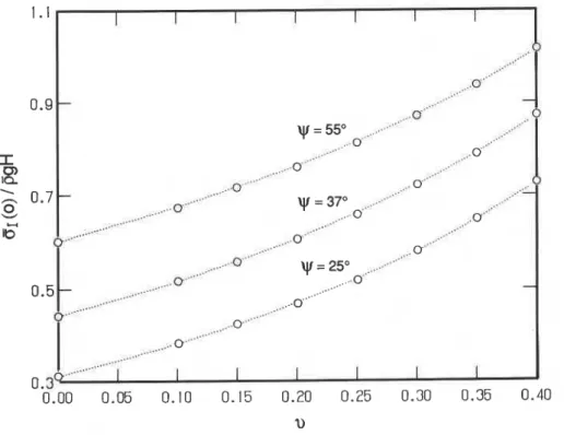
Fig. 3. Maximum principal stress as a function of v and y for the traction-free boundary condition. D*=O. (...) model; ( 0 ) finite-element calculations.

PRESSURES

pirical relation for L I H with the traction-free cent. Figure 3 gives examples for D*=0.0. For the

boundary condition is: traction-free condition the resultant force is per-

L

v

pendicular to the face of the structure.

---0.27+-

H- 12 (11) _HaefeliEquation 12 is similar in form to that given by

( 1948). He called the first term the dy- With Eqs. 1 1 , 9 and 10 the depth-averaged value of namic component of pressure and the second term eX(O) (or the maximum principal stress, ~ ~ ( 0 ) ) is: the static component. The second term of Eq. 12 is identical to Haefeli's formulation but only for the restricted case of the traction free boundary condition (not specified by Haefeli). The first term of Eq. 12 differs substantially from Haefeli's ( 12 expression.

The two terms in Eq. 12 result from gravity loads applied parallel and perpendicular to the slope respectively. The terms may be calculated separately by application of gravity loads (body forces) in these directions. Equation 12 was derived from solutions in the ranges 25" I t + ~ < 55", 0 l u 1 0 . 4 and 0 I D * / H I 3 (see McClung, 1982, for a discussion of these ranges). The solutions compare with two- dimensional finite-element results within a few per-

0 0 0 1 . 1 0.9 I 0 IQ \

-

0.7 0 w

No-slip boundary condition

0.00 0.05 0.10 0.15 0.20 0.25 0.30 0.35 0.40 I I I

I

I I I ,..,.' ... .I.. ,.,- ,..a"' ....

-

... 6'" _... y j = 5 S 0 .... ,..' ,..@.-' ,..' ... ... ... 0.' ...

,...o.'"'

..I' ... . .'o..". " .,,. _0."' ... _._.I.

-

yj = 370 ...~.." ... ~ - . " ' ' ' ... ... _....... -0'" .... .... ... .,.0.." ... 0"" _... ... _...

Field data show that, in general, the resultant force is not perpendicular to the face of the structure (e.g. Kiimmerli, 1958). This result is expected physically: if slip along the structure is inhibited, shear forces will be present there causing the resultant force to have a component perpendicular to the slope. In general, the face of a structure will not be .._..' .... 0.'-- .... ... 0""' _{yj =}_25" _... ... ... 0.-"" ...

..o"

... 0.5 IS

e

-

.. ". ... ._.. _{,_..-.},... .... 0. ... '.'"" ..,@"'. ... ... ... 0."'

...

L....

...> 1 I I I I I 1 0.3

(9)

completely traction-free and we feel the no-slip

boundary condition (u = v= 0 ) is a closer approxi-

mation to conditions encountered in the field ex- cept when the snowpack is melting rapidly.

Numerical solutions show that the no-slip condition is more complex to model than the traction- free condition. Not only are shear forces produced on the structure, but the normal forces in the vicin- ity of the structure are significantly reduced from their values without a wall present; a simple esti- mate such as Eq. 10 is not available.

The shear stress on the structure may be estimated from Eq. 3:

Since u=O all along the structure, Eq. 13 may be depth averaged to give the average shear stress on the structure:

There is no simple method to evaluate Eq. 14 and it is not compatible with the glide boundary condition. Similar to Eq. 8, the depth-averaged equilibrium equation in the z-direction yields a value for the average vertical stress (after some algebra):

Evaluation of Eq. 15 at the structure gives:

aZ(O) = 4PgH cos y / - 4pH

(z)x=o

-

In common with Eq. 14, there is no simple method to evaluate Eq. 16 from a one-dimensional model. Similar to Eq. 7, an expression for the vertical stress on the plane perpendicular to the face of the structure can be derived (using v=O at x=O) from Eq. 3:

Substituting Eq. 16 into Eq. 7 gives a form for ex(o):

We have evaluated Eq. 18 numerically using finite- element solutions to get an approximate empirical

expression for ex(0). If the form of Eq. 12 is re-

tained, L / H is given by:

to complete the definition of &(0) in Eq. 12. An approximate empirical expression for T(O) from numerical evaluations derived similar to Eq. 19 is:

Equations 12, 19, 17 and 20 complete the defini- tions of stresses at the structure for no-slip boundary condition. The maximum compressive (principal) stress can be estimated by standard methods:

A related quantity of interest is direction of the maximum compressive stress. From standard theory, the (downward) angle that the maximum principal stress deviates from the x-axis is:

p=

tan-' ( ~ x ~ ~ ~ ~ ? z ~ ~ ~ )

Equations 2 1 and 22 may prove useful in design ap-

plications. Assuming y/= 37 "

,

and Bader's data

( v x O for low density snow; v=0.25 for dense

snow) we get /3=25.5" and 20.5". Therefore, the maximum compressive force direction is estimated to vary from 0" (perfectly smooth or wetted structure) to about 25" (rough structure) downward

from the x-axis (for y/= 37 " )

.

Equations 21 and 22 should be used cautiously: they are not as accurate as Eqs. 11 and 12 for the traction-free boundary condition and therefore fi-

(10)

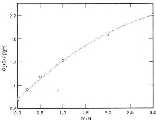
Fig. 4. Maximum principal stress as a function of D*for y/=4So, v=0.25. (....) model; ( 0 ) finite-element calculations. The no- slip boundary condition is assumed.

nite element or other numerical procedures are preferable. Errors of up to 15% may be expected in calculations of individual estimates of stress components such as f(0). Errors for 4 ( 0 ) , @,(O), and C ( 0 ) are generally less than 10%. Figures 4 and 5 compare the results of Eq. 2 1 with two dimensional numerical solutions. Figure 6 compares the predictions of Eqs. 12 and 21 and the estimates of &(O) for the extremes in boundary conditions. This comparison shows @,(O) is higher for the traction-free boundary condition with a greater deviation at low slope angles and low values (the difference is about 25% for y/=25" ).

When a structure is erected perpendicular to the slope (see Fig. 2), the stress components of interest are 6,.(0) and f(0). The magnitude of the resultant force (per unit area) is:

The ratio in Eq. 24 has been estimated in the field

(Kiimrnerli, 1958). Salm ( 1977) gives a range for

tan t from field measurements ( y/= 37 "; D* = 0):

tan e x 0.7 for low density snow and tan E % 0.3 for

high density snow. From Bader's data (Salm, 1977),

with v=O.O (low density snow) and v=0.25 (high

density snow) calculations with Eqs. 12, 19 and 20

give tan e = 0.6 1 and 0.29 respectively for our model;

finite-element calculations give tan t = 0.77

(v=O.O) and tan t=0.36 (v=0.25). The agree- ment is surprisingly good for the constant viscosity, constant (depth averaged) density case.

PROPERTIES OF FIELD DATA FROM WESTERN NORWAY

OR = [~,(O)'+Z(O)~] i ₍₂₃₎ The previous section provides simple estimates

for pressures with snow deformation taken as a lin-

and the direction may be ddined (e.g. Haefeli, _{ear viscous material. In this section, field data are}

1948): _{introduced to illustrate how pressures depend on}

tan ~ = 1 ( 0 ) / 8 ~ ( 0 ) (24) snowpack properties. Our data consist of maxi-

(11)

1

.o

0.9

5

0.8 la

-.

n 0 V 0.7

o.

6L 0.5 I I I I I I I

-

o :",,

-

./". 0 ,.-" ...

-

0 _...

-

... .... (.," _.." ... 0 ... ... > _...... -.,. ...

-

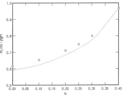
I I I I I I I 0.00 0.05 0.10 0.15 0.20 0.25 0.30 0.35 0.40 2)

Fig. 5. Maximum principal stress as a function of v for yl=45", the no-slip boundary condition and D*=0. (...) model; ( 0 )

finite-element calculations.

-

0.0 0. I 0.2 0.3 0.4 I

2)

Fig. 6. Comparison of a X ( O ) as a function of v and y for the analytical model. ( . O . ) traction-free boundary condition; (. . )

(12)

the centre of a 15 m long avalanche defence structure erected perpendicular to the slope. The incline

at the site is nearly constant (25" ) for a long dis-

tance upslope from the structure and the ground surface is fairly smooth rock behind the structure.

Previously (Larsen et al., 1985 ) the field measure-

ments were described in detail. Supporting field measurements include a set of indexes for snow-

pack properties: H (average snowdepth), ?= (aver-

age snowpack temperature) and S (average snow-

pack stiffness). The parameter S is defined as the

total energy (joules) to drive a ram penetrometer vertically through the snowpack. The values of am and a, were estimated from strains measured in the steel supporting beams of the structure (McClung et al., 1984).

In the 1985 paper, a regression analysis was pre- sented to describe am and a, in terms of measured field parameters. We now present a similar analysis with an expanded data set (four more winters of data).

For a, the best relation found is:

The descriptors are: r is correlation coefficient, S, is

standard error, and N is number of data points. If pgH is excluded as a variable, the best relation is:

In Eq. 26, the t statistic is 6.5 for In S a n d 2.5 for

T.

With pgH in the analysis, no significant improve-

ment was gained by addition of

T,

ln

T,

s

or In

S

in

a multiple-regression analysis; the resulting equations were found to be overfitted.

For a,, the best expression is a power law rela-

tion with respect to pgH:

Without pgH the best relationship is:

For Eq. 28, the t statistic is 2.3 for

?=

and 5.1 for

In S. WithpgH in the analysis, estimates forpgH are

not improved with a multiple-regression analysis using the other variables.

The best relationship among the snowpack indexes was found to be:

r2=0.64, Se =0.19, N=46

1

(29)

In Eq. 29, In has a t statistic 8.6 and

?=

has a t

statistic 4.2. This relationship indicates that the effects of temperature and stiffness are largely con- tained in pgH.

The best relation between a, and a, is a linear

one:

a, = 1.5 a,-0.60 kPa

r2=0.91,S,=1.36,N=55

Expression 30 shows that am FZ 1.5 a, to a good ap-

proximation. We will subsequently show that this important feature of the data cannot be explained with a constant stiffness, depth-averaged model. It may be noted in Eq. 30 that the constant is not very

significant: the t statistic for a, is 22.5 and for the

constant it is

-

1. Without the constant a regression

analysis gives a,= 1.5 a,. Similar comments apply

to Eqs. 23 and 25.

COMPARISON WITH FIELD DATA

Two sets of field data exist for the plane-strain problem but they differ in snowpack properties and measurement techniques. Our data set is taken from a relatively low altitude, high latitude site in western Norway. The other data set was taken from a 37" slope in Switzerland (Kiimmerli, 1958). For both data sets, the glide component is negligible

(U=D*=O).

Due to climate variations, it is possible that the snowpacks for the two data sets differ. We suspect that one principal difference may be with respect to snowpack stiffness. Our data are subject to unu- sually strong windpacking effects; this can create a stiffer snowpack. The data from Switzerland (lower latitude, higher altitude) may be influenced more by the effect of solar radiation exposure but we are

(13)

unsure of this. The lower slope angle for our loca-

tion (25" ) should introduce a greater settlement

component into the snow deformation promoting higher densification and increased stiffness.

Both data sets contain forces in addition to those perpendicular to the structure. In particular, the data from Switzerland show clearly that the resultant force is not perpendicular to the structure. This indicates the presence of shear forces and very little slip on the face of the structure. The condition is expected physically and therefore we believe the no- slip boundary condition will be the more realistic of the two extremes. Since shear forces appear in the data it is more realistic to compare the measure-

ments with @, than with @, in general.

The data from Switzerland are taken by measuring spring displacements to infer forces perpendicular and parallel to a structure placed perpendicular to the ground. Therefore, the magnitude of the resultant is the proper quantity to compare with. The data from Norway were determined largely by axial forces and the structure is slightly inclined downslope from the perpendicular but we feel a, in Eq. 23 is the best quantity to compare with. For the

traction-free boundary condition, @I=

ax

from Eq.

12 is the analogous quantity.

Consider first the average pressure, OR, on the face

of the structure. For the no-slip boundary condition, linear deformation and the other conditions defined in Fig. 2, the ratio o,/pgH should only de-

pend on u and ty. From data reviewed by Salm

( 1977), we regard the extreme range of v to be O-

0.4 for the depth-averaged density range of the data sets (200 kg m-3 to 600 kg m-3).

Finite-element calculations show that the mean

value of our data (o,/pgH= 0.64; ty= 25" ) implies

u x 0.4 and range 0-0.45 (no-slip boundary condi-

tion). For the Swiss data (37" slope), the mean

value (o,/pgH= 0.58 ) implies a mean value u x 0.2

for the data set, which is a very reasonable value (according to Bader's data) for the density range of the experiments. However, while the implied mean

value for u seems appropriate, many of the data im-

ply negative values for u; this seems unlikely according to the Poisson ratio data reviewed by Salm. Figures 7 ( y = 2 5 " ) and 8 (ty=37") show comparisons of o, (in kPa) from the data with finite- element conditions for constant density and viscos-

ity for the extreme (expected) range of u (0-0.4).

From Figs. 7 and 8, it can be seen that the scatterband of the data sets is wider than the band of predictions for this model. As a percentage of the mean value, the standard deviations of o,/pgH for the

data sets are nearly identical [21°/o ( ty= 25" ); 23%

( ty= 37" )

1.

An important limitation of the model

appears: the prediction range is smaller than the data scatterbands.

Another result (Fig. 7) is that the constant density-stiffness model underestimates the mean of our

pressure data by at least 20% assuming values for u

near the middle of Bader's range. This result does not change very much even if we consider vertical

stresses 13~ and compare our data with 6, rather than

a,.

From Fig. 8, it appears that the constant den-

sity-stiffness model overestimates some of the pressure data on the 37" slope (unless negative val-

ues for Y are admitted).

Numerical calculations were performed to ex- plore depth-dependent density variations. Assum- ing a linear increase in density with depth, these results showed almost no effect on average pressure, or the maximum pressure for either the no-slip or traction-free boundary condition. In combination with previous comparisons, these results imply that variations in snowpack stiffness will be required for a complete explanation of the snowpressure data.

Linear depth variations in snowpack stiffness may be analyzed with viscosity data summarized by

Haefeli ( 1967). He showed that the shear viscosity

of snow varies by approximately two orders of mag-

nitude for densities from 300-500 kg m -3. In this

density range, Haefeli gives values for p from 10"-

1 012 kg (m sec) - I . Figures 9 and 10 compare nu-

merical calculations with our data using these val-

ues and u constant in the range (0-0.4); constant u

implies shear viscosity and bulk viscosity increase with the same depth dependence.

With depth dependent stiffness, numerical calculations show that snowpressure is nearly independent of the magnitude (mean value) of the viscosity used but it is sensitive to the form of the depth dependence chosen. With linear variation in shear

stiffness ( u taken constant) the pressures are nearly

independent of the magnitude of the stiffness gra- dient taken.

(14)

SNOW CREEP

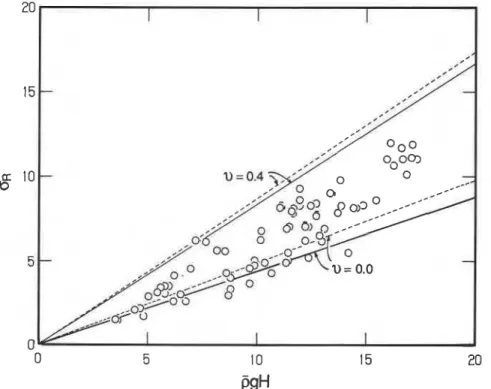
Fig. 7. Resultant pressure (kPa) as a function of pgH (kPa) for data from Norway. ( 0 ) experimental data. Finite-element calculations are shown for the extreme range of v and the extremes in boundary conditions. y/=25", D*=0. (---) traction free;

(-) no slip.

(15)

20 I I I- I > 15

-

0 0 o,," 0 ,.*'

6

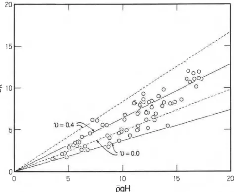
10-

Fig. 9. Resultant pressure data (kPa) from Norway as a function of pgH (kPa). In this example both stiffness and density are taken to increase linearly with depth, otherwise the assumptions are the same as in Fig. 7. (---) traction free; (-) no slip.

0 5 10 15

PgH

(16)

SNOW CREEP PRESSURES

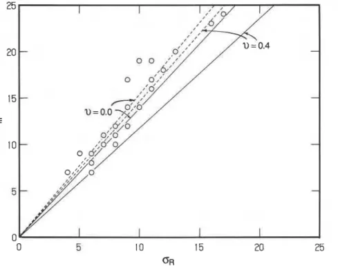
Fig. 11. Maximum pressure versus resultant pressure (both in kPa) for data (0 ) from Norway. Finite-element calculations for no-slip boundary condition are given for: (-) constant density-viscosity model; and (---) density and viscosity linear with depth (both take D*=0 and ~ = 2 5 " ).

For linear increase in stiffness and density with depth, the values a,/pgH and aR,pgH decrease sub- stantially from their values when stiffness and density are taken constant. For y/= 25", aR/pgH in-

creases from 0.29 to 0.53 for linear variations and no slip as u increases from 0 to 0.4. The correspond- ing values for p and p constant are 0.40 and 0.68. These results may be compared with a mean value of the ratio (0.64) for our data. For y/= 37", linear

depth dependence of stiffness and density gives a,/

pgH in the range 0.37-0.64 for the no slip boundary condition. For constant density and stiffness the corresponding values are 0.49 to 0.84. The mean value for the measured ratio from this slope angle is 0.58.

From Figs. 9 and 10, it is clear that the depth dependent density-stiffness model underestimates many of the data for either set. Also, similar to the constant density-viscosity model, the spread of predictions is smaller than the data scatterband for either data set. We conclude neither model pro-

vides a satisfactory description of the data.

Our data contain information about the maximum pressure on the structure. Figure 1 1 shows om

versus a, (both in kPa) and comparison of predictions of the two models from finite-element calculations. From Eq. 29, the mean of the data implies

a m / a R = 1.5 to a good approximation. For the constant density-viscosity model, the calculated ratio declines from 1.39 to 1.18 as u increases from 0 to 0.40 (no-slip boundary condition). The ratio de- creases from 1.54 to 1.46 for the same range of u for the linear depth-dependent density-stiffness model thus providing an excellent fit to the mean of data. If maximum compressive stress a, ( 0 ) is used in the ratio amla, (0 ) , the no-slip boundary condition gives 1.47 nearly independent of u assuming linear depth- density and stiffness variations as above. For the traction-free boundary condition ,(constant density and stiffness) the ratio declines from 1.43 to 1.1 1

(17)

SUMMARY AND DISCUSSION

Our reformulation of the constant viscosity-constant density one-dimensional treatment of the plane strain snowpressure problem is of both historical and practical interest. The solution represents the analytical model first sought by Haefeli (Bader et al., 1939) in his doctoral thesis. Also, our analytical model is of practical interest since it allows the average pressures to be roughly estimated using a hand calculator. It appears that this simple model underestimates our measured field data by about 20%.

The model does not account for initial stresses. Instead, the long term loads on the structure are defined in terms of viscous stresses and strain rates. These assumptions have a long history in snow mechanics (Bader, 1962; Mellor, 1975). We feel that our new model represents a more accurate repre- sentation of the linear problem than our previous attempts which included initial stresses.

Comparison of field data with the two density- stiffness models shows that neither provides a com- prehensive explanation of the data. It is surprising that the mean value of oR/pgH is higher for the 25" slope (0.64) than it is for the 37" slope (0.58). Lin- ear regression of the Swiss data gives o,= 0.69

pgH- 1.05 (kPa) which is nearly identical to Eq. 25 for the data on the 25" slope. For the same snow properties, we believe that the mean value of pressure should increase with slope angle if snow is modelled as a linear material. Therefore, either the snow properties are significantly different for the two sites or the deformation conditions affect stiffness variations greatly with slope angle or both. The site in Norway has a very stiff mid-winter snowpack due to windpacking and a minimum effect from solar radiation. Also, the lower slope angle at the site should produce a greater settlement component to increase stiffness. These effects could combine to give pressures as high as those in Switzerland even though the slope angle is higher for the latter by 12". Our analysis of the ratio o,,,/aR further highlights the importance of stiffness variations: we were un- able to explain the ratio until depth-dependent stiffness variations were introduced.

Since density variations alone do not provide a consistent match to field data, we believe that variations in stiffness (non-linear viscous relations)

may be the key. Our attempt to vary stiffness (linear increase with depth) is the simplest consistent with snow deformation properties in the field. For well settled snow, field-creep experiments data show the shear strain rate is approximately independent of depth (Mellor, 1975; McClung, 1975) and this implies the shear stiffness increases with the same depth dependence as the shear stress (on open slopes). It is of further interest that creep experiments for well settled snow indicate effective values for v in the range 0.23-0.38 (McClung, 1975) for final densities (500-550 kg m-3) and these values are in excess of Bader's estimates from laboratory experiments. If lower values for the effective ratio of shear to bulk viscosity (higher effective v) are appropriate in the field (as opposed to the laboratory) our conclusions may be altered when stiffness

variations are considered. Salm ( 1977 ) provides

some motivation for the belief that effective values for u may be higher when non-Newtonian behav-

iour takes places. Numerical calculations of tan 6 in

Eq. 24 show that tan 6 increases when density and

stiffness increase linearly with depth. Therefore, higher effective values for u are also implied to match the field data of Kiimmerli (1958) if stiffness varies linearly with depth.

Until a proper non-linear deformation law is for- mulated (and applied), the importance of stiffness variations will not be defined. Based on our data, we recommend a safety factor of at least 25% over predictions of the analytical model (constant stiffness) when traditional values for v (e.g. Bader et

al., 195 1 ) are applied. For maximum pressure, we

believe the values should be 50% higher than pre- dicted average pressures.

ACKNOWLEDGEMENTS

We are grateful to Krister Kristensen for assis- tance with the field measurements. We also wish to thank the Norwegian Water Power and Electricity Board for funding part of the project.

REFERENCES

Bader, H., 1962. The physics and mechanics of snow as a ma- terial. In: J. Sanger (Editor), Cold Regions Science and

(18)

Engineering, Part 11, Section B. U.S. Army CRREL, Han- over, N.H.

Bader, H., Haefeli, R., Bucher, E., Neher, J., Eckel, O., Thams, C. and Niggli, P., 1939. Der Schnee und seine Metamor- phose. Beitrage zur Geologie der Schweiz. Geotech. Ser., Hydrol., Lief. 3. (English translation: U.S. Snow, Ice and Permafrost Research Establishment, Translation 14, 1954.)

Bader, H., Hansen, B.L., Joseph, J.H. and Sandgren, M.A., 195 1. Preliminary investigations of some physical properties of snow. U.S. Snow, Ice and Permafrost Research Establishment, Rep. 7.

Haefeli, R., 1948. Schnee, Lawinen und Gletscher. In: L. Bendel (Editor), Ingenieur-Geologie. 2. Bd. Springer, Wien, pp. 663-735.

Haefeli, R., 1967. Some mechanical aspects on the formation of avalanches. In: H. Oura (Editor), Physics of Snow and Ice, Vol. 1, Part 2. Proc. Int. Conf. Low Temperature Sci- ence, Inst. Low Temperature Science, Sapporo, pp. 1 199- 1213.

Kamb, B., 1970. Sliding motion of glaciers: theory and obser- vation. Rev. Geophys. Space Phys., 3(4): 673-728. Kiimmerli, F., 1958. Auswertung der Druckmessungen am

Druckapparat Institut (DAI). Inter Bericht des Eidg. Inst. Schnee- und Lawinenforschung, Nr. 240.

Lang, T.E. and Nakamura, T., 1984. Finite element computer analysis of snow settlement. Res. Notes Natl. Center Dis- aster Prevention, 59.

Larsen, J.O., McClung, D.M. and Hansen, S.B., 1985. The temporal and spatial variation of snow pressure on structures. Can. Geotechn. J., 22: 166-171.

McClung, D.M., 1975. Creep and the snow-earth interface condition in the seasonal alpine snowpack. IAHS-AISH Publ., 114: 236-248.

McClung, D.M., 198 1. A physical theory of snow gliding. Can. Geotech. J., 18: 86-94.

McClung, D.M., 1982. A one-dimensional analytical model for snow creep pressures on rigid structures. Can. Geo- tech. J., 19: 401-412.

McClung, D.M. and Clarke, G.K.C., 1987. The effects of free water on snow gliding. J. Geophys. Res., 92 (B7): 6301- 6309.

McClung, D.M., Larsen, J.O. and Hansen, S.B., 1984. Com- parison of snow pressure measurements and theoretical predictions. Can. Geotech. J., 21: 250-258.

Mellor, M., 1975. A review of basic snow mechanics. IASH- AISH Publ., 114: 251-291.

Reiner, M., 1946. The coefficient of viscous traction. Am. J. Math, 68: 672-680.

Reiner, M., 1949. On volume - or isotropic flow as exempli- fied in the creep of concrete. Appl. Sci. Res., Ser., A ( 1 ): 475-488.

Salm, B., 1967. An attempt to clarify triaxial creep mechanics of snow. In: H. Oura (Editor), Physics of Snow and Ice, Vol. I, Part 2. Proc. Int. Conf. Low Temperature Science, Inst. Low Temperature Science, Sapporo, pp. 867-874. Salm, B., 1977. Snow forces. J. Glacial., 19 (81 ): 67-100.

(19)

Research in Construction. A list of building practice and research publications available from the Institute may be obtained by writing to the Publications Section, Institute for Research in Construction, National Research Council of Canada. Ouawa, Ontario, KIA

0R6.

Ce document est distribu6 sous forme de tir6-8-part par I'Institut de recherche en construction. On peut obtenir une liste

des

publications de I'Institut portant sur les techniques ou les recherches en matihe de b%timent en krivant

B

la Section des publications, Institut de recherche en construction, Conseil national de recherches du Canada. Ottawa (Ontario), KIA 0R6.