CAPTURING THE IMPACT OF MODEL
ERROR ON STRUCTURAL DYNAMIC
ANALYSES DURING DESIGN EVOLUTION
by
Alissa Naomi Clawson B.S., Aerospace Engineering
Boston University, 1999
SUBMITTED TO THE DEPARTMENT OF AERONAUTICS AND ASTRONAUTICS IN PARTIAL FULFILLMENT OF THE REQUIREMENTS FOR THE DEGREE OF
MASTER OF SCIENCE
IN AERONAUTICS AND ASTRONAUTICS at the
MASSACHUSETTS INSTITUTE OF TECHNOLOGY August 24, 2001
AERO
MASSACHUSETS NSTITUT OF TECHNOLOGYAUG
13
2002
LIBRARIES
@ 2001 Massachusetts Institute of Technology. All rights reservedSign e. . . . . . . . . .
Alissa N. Clawson, Department of Aeronautics and Astronautics
August 24, 2001
Certified by ... .. .. .. .. .. .. .. .. ..
David W. Miller, Assistant Professor of Aeronautics and Astronautics Thesis Supervisor Signature of Author .. .
i
1
.10 AA ccepted by .. .. .. .. .. .. ... . .. . . . .. . . . . . ... .. .. ... .
Wallace E. Vander Velde, Professor of Aeronautics and Astronautics Chairman, Department Graduate Committee
ANAL-Capturing the Impact of Model Error on Structural
Dynamic Analyses During Design Evolutionby
ALISSA NAOMI CLAWSON
Submitted to the Department of Aeronautics and Astronautics on August 24, 2001 in Partial Fulfillment of the
Requirements for the Degree of
Master of Science in Aeronautics and Astronautics
ABSTRACT
Space telescopes are complex structures, with stringent performance requirements which must be met while conforming to design constraints. In order to ensure that the perfor-mance requirements are met, accurate models of all the different components of the inte-grated model is needed. In modeling the structure, however, early in the project, the design is not complete when analysis starts and key design decisions are made. Knowledge of how the model fidelity evolves as the design or model improves helps with the interpreta-tion of the analysis such that only the appropriate informainterpreta-tion from the data will be used. In this thesis, model fidelity evolution is studied to understand what key information can be gathered at the different stages of fidelity and what error types to expect. First, a simple truss problem is used as an example of the different stages of model fidelity by using four different types of models: Bernoulli-Euler beam, Timoshenko beam, truss with rod mem-bers and truss with bending memmem-bers. Then, the Origins Testbed is used as an example of a completed design to parallel model updating error to design fidelity error. Finally, the ARGOS testbed is introduced as a low fidelity model. The conclusions drawn from the Origins Testbed and example problem are applied to the results of a disturbance analysis of ARGOS.
Thesis Supervisor: David W. Miller
ACKNOWLEDGMENTS
I would like to thank (NOT in order of importance):
e the U.S. Navy for the FY99 scholarship that allowed me to work for my Masters Degree (and for letting me fly),
e my parents for encouraging their children to be intelligent, independent, and hard working people,
e my friends for persuading me to not study ALL the time,
e the SSL for being an awesome group of students, faculty and staff, who all made life at MIT fun,
e Becky Masterson, who (who's "who"?) probably has this (what does "this" mean?) entire thesis memorized,
e the PIT crew for just being,
e my BU girls for being the sisters I never had,
e my advisor, Prof. Miller, for directing my thesis,
e and Prof. JP Clarke for helping me in the beginning when I was lost in the shuffle.
TABLE OF CONTENTS
... 3 Acknowledgments Table of Contents List of Figures . . . List of Tables . . . Nomenclature . . . . . . . .. . . 5 . . . . .. . . 7 . . . . .. . . 9 Chapter 1. Introduction . . . . . 1.1 Background . . . . 1.1.1 NASA Origins Program1.1.2 Space Telescope Stringent Performances 1.2 Integrated Modeling . . . . 1.3 Thesis Objective . . . . 1.3.1 Importance of Accurate Structural Models 1.3.2 Model Fidelity . . . . 1.4 Dynamics Optics Controls Structures (DOCS) .
1.5 Thesis Overview . . . .
Chapter 2. Sample problem . . . . 2.1 State Space Representation . . . . 2.2 Problem Formulation . . . . 2.2.1 Equivalent Inertia . . . . 2.2.2 Continuous Beam Solutions . . . . 2.2.3 Timoshenko Beam . . . . 2.2.4 Non-homogenous Analysis . . . .
2.2.5 Conclusions . . . . Chapter 3. Origins Testbed . . . .
3.1 Background . . . . 3.2 General Description . . . . . . . . 9 1 . . . . 9 1 . . . . 9 1 7 Abstract 13 15 19 19 19 24 27 30 30 31 34 36 39 39 46 47 55 59 81 89 . . . . . . . . .
8 TABLE OF CONTENTS
3.2.1 Optics . . . . 93
3.3 Modeling . . . . 93
3.4 Modeling the Origins Testbed . . . . 95
3.4.1 Model Evolution . . . 102 3.4.2 System Identification . . . 106 3.5 Summary . . . 110 Chapter 4. ARGOS . . . 113 4.1 Description of ARGOS . . . 114 4.1.1 Architecture . . . 114 4.1.2 Optics . . . 115
4.1.3 Attitude Control System . . . 119
4.1.4 Structure . . . 120
4.2 ARGOS Integrated Model . . . 124
4.2.1 Structural Dynamics . . . 125 4.2.2 Disturbance M odel . . . 127 4.2.3 Optical Sensitivity . . . 132 4.3 Disturbance Analysis . . . 135 4.4 Summary . . . 138 Chapter 5. Conclusion . . . 139 5.1 Summary . . . 139 5.2 Conclusions . . . 140 5.3 Future Work . . . 141 References . . . .1 143
LIST OF FIGURES
Figure 1.1 Figure 1.2 Figure 1.3 Figure 1.4 Figure 1.5 Figure 1.6 Figure 1.8 Figure 1.7 Figure 1.9 Figure 1.10 Figure 2.1 Figure 2.2 Figure 2.3 Figure 2.4 Figure 2.5 Figure 2.6Timeline of the Universe . . . . Space Telescope Timeline . . . . Next Generation Space Telescope -GSFC Design Space Interferometry Mission . . . . Example Integrated Model: SIM . . . . block diagram representation of precision controlle
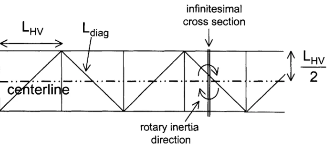
. . . . 2 0 . . . . 2 1 . . . . 2 2 . . . . 2 5 d . . . . opto-structural inte-grated model Uncertainty [Gutierrez, 1999] . . . . Model Fidelity Evolution . . . . DOCS Flowchart . . . . Thesis Roadmap . . . . Simple system . . . . Example problem truss schematic . . . . . Labeling of the truss (left four bays shown) Axial Compression . . . . Bending Moment . . . . Shear Force . . . . 28 28 . . . . 3 3 . . . . 3 3 . . . . 3 5 . . . . 3 7 . . . . 4 0 . . . . 4 7 . . . . 4 9 . . . . 5 1 . . . . 5 2 . . . . 5 3 Figure 2.7 Rotary inertia per unit length is equivalent to the inertia of the truss
calcu-lated about the centerline, rotating in and out of the plane divided by the total
length . . . . 54
Figure 2.8 Truss modeled as beam . . . . 56
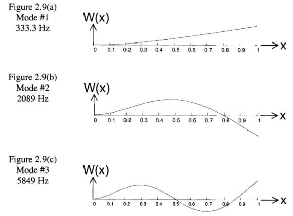
Figure 2.9 First three mode shapes for continuous Bernoulli-Euler beam . . . . . 60
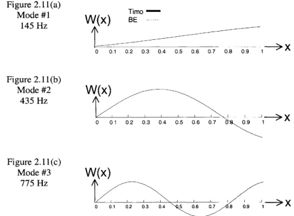
Figure 2.10 Deflection for Timoshenko beam [Meirovich, 1997] In a Bernoulli-Euler beam , $ = 0. . . . . 61
Figure 2.11 Mode shapes of canti levered Timoshenko beam (with BE beam) . . . 65
Figure 2.12 rod with axial forces . . . . 66
Figure 2.13 degrees of freedom for BE beam in bending . . . . 69
Figure 2.14 Bernoulli Euler (40 elements) -modes shapes . . . . 73
Figure 2.15 Bernoulli-Euler Beam (8 elements) -mode shapes . . . . 73
9
10 LIST OF FIGURES Figure 2.16 Figure 2.17 Figure 2.18 Figure 2.19 Figure 2.20 Figure 2.21 Figure 2.22 Figure 2.23 Figure 2.24 Figure 2.25 Figure 2.26 Figure 2.27 Figure 2.28 Figure 2.30 Figure 2.29 Figure 3.1 Figure 3.2 Figure 3.3 Figure 3.5 Figure 3.4 Figure 3.6 Figure 3.7 Figure 3.8 Figure 3.9 Figure 3.10 Figure 3.11 Figure 3.12 Figure 3.13 Figure 4.1 Figure 4.2
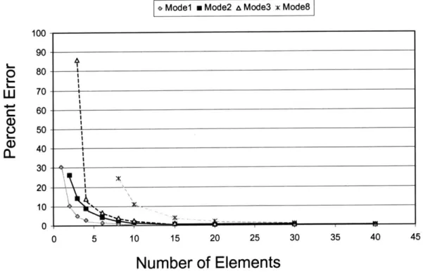
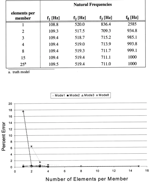
percent error of BE-beam FEM mode compared to continuous BE-beam verses number of elements . . . . Timoshenko beam (40 elements) -mode shapes . . . . Percent error of Timoshenko finite element models . . . .
Truss with rods - mode shapes . . . .
Truss with bending beams, higher mode . . . . Percent Error of Bar Truss modes vs. number of elements per member BE beam SYS ID . . . . Timoshenko beam transfer function . . . . Truss with rod members SYS ID . . . . Truss with Bending members SYS ID . . . . Truss with bending members -zoom . . . . Comparison of all four types . . . . Truth model and Bernoulli-Euler beam transfer functions . . . . Rod truss, bar truss with 1 element per member and truth model . . . . Truth model and Timoshenko beam transfer functions . . . . Origins Testbed . . . . Origins' truss structure . . . . Truss strut modeling [Mallory, 1998] . . . . Schematic of counter-weight placement looking down on top of the base
100
B ase . . . . Truss only . . . . Computer image of Origins Testbed -iteration 3 . . . . Two modes of Origins 3 . . . . View of constraints on Origins 7 . . . . Origins 11 Mode Shapes . . . . System Identification of the Origins Testbed -Experimental Data . . . Origins 7 Transfer Functions . . . . System ID of Origins version 11 . . . . Golay-3 configuration . . . . Relay Optics Schematic -dimensions in mm . . . .
74 76 76 78 79 80 82 83 84 85 85 86 87 88 88 92 96 97 100 103 104 105 105 107 108 109 111 116 118
LIST OF FIGURES 11 Figure 4.3 Figure 4.4 Figure 4.5 Figure 4.6 Figure 4.7 Figure 4.8 Figure 4.9 Figure 4.10 Figure 4.11 Figure 4.12 Figure 4.13 Figure 4.14 Figure 4.15 Figure 4.16 Figure 4.17 Figure 4.18
ARGOS structural design . . . . Air Bearing Support Beam Clearance . . . . Telescope Collar . . . . The three bending directions the support beams must counter . . . Side view of subaperture and center bus geometry . . . . A ssem bly . . . . Subaperture and Center Bus . . . . First Mode Shape [52.7 Hz] . . . . Reaction Wheel Imbalance Representation . . . . B-Wheel Disturbance PSD's in Wheel Frame . . . . Euler Angles (s/c denotes spacecraft frame; w denotes wheel frame) [G utierrez, 1999] . . . . Reaction wheel orientation . . . . Example calculation of optical path length sensitivity . . . . Ray trace for sensitivity calculation . . . . PSD and cumulative RMS for ARGOS . . . . High frequency mode shapes for ARGOS . . . .
121 . . 121 . . 122 122 123 125 . . 126 127 128 130 131 132 134 135 136 138
LIST OF TABLES
TABLE 2.1 TABLE 2.2 TABLE 2.3 TABLE 2.4 TABLE 2.5 TABLE 2.6 TABLE 2.7 TABLE 2.8 TABLE 3.1 TABLE 3.2 TABLE 3.3 TABLE 3.4 TABLE 3.6 TABLE 3.7 TABLE 3.5 TABLE 3.8 TABLE 3.9 TABLE 4.1 TABLE 4.2 TABLE 4.3 TABLE 4.4 TABLE 4.5 TABLE 4.6 TABLE 4.7 TABLE 4.8Truss property values . . . . 4 8 Equivalent beam properties ...
Continuous Bernoulli-Euler Beam ...
Modes for continuous equivalent Timoshenko beam Bending modes of the BE beam FEM ... Timoshenko beam FEM modes ... Truss with rods ...
Truss with Bending Beams ... Truss struts ... ... Reaction Wheel ... Brass Appendages ...
Base Fram e ... ... .. . .. Point M asses ... ... .. . .. Material Properties [Gere, 1997] . . . .
Counter-weight masses . . . . Origins 11 M odes . . . . Overview of Origins Model Evolution via Engineering Mission Success Criteria (from PDR) . . . . Takahashi properties . . . . Relay O ptics . . . . Beam Combiner . . . . Structural Dimensions . . . . Ithaco B Wheel Model [Masterson, 1999] . . . . ARGOS wheel Euler angles . . . . Critical M odes . . . . . . . . 55 . . . . 59 . . . . 64 . . . . 72 . . . . 75 . . . . 78 . . . . 80 . . . . 97 . . . . 98 . . . . 98 . . . . 99 . . . 101 . . . 101 . . . 10 1 . . . . 106 Insight . . . . 112 . . . . 113 . . . . 116 . . . 117 . . . . 118 . . . 124 . . . 129 . . . . 132 . . . 13 7 13
NOMENCLATURE
Abbreviations
AFRL Air Force Research Laboratory
ARGOS Active Reconnaissance Golay-3 Optical Satellite
BE Bernoulli-Euler
CCD Charged Couple Device
CDIO Conceive, Design, Implement, Operate CG center of gravity
COBE Cosmic Background Explorer
DOCS Dynamics, Optics, Controls, Structures dof degree of freedom
FE Finite Element
FEM Finite Element Model FRF frequency response function FOV field of view
GSFC Goddard Space Flight Center GUI Graphical User Interface
IEEE Institute of Electrical and Electronics Engineers ISO Infrared Space Observatory
ISS International Space Station LBT Large Binocular Telescope
MACE Middeck Active Control Experiment MIT Massachusetts Institute of Technology MTF Modulation Transfer Function
NASA National Aeronautics and Space Administration NGST Next Generation Space Telescope
NICMOS Near Infrared Camera and Multi-Object Spectrometer NRO National Reconnaissance Office
OPD Optical Path-Length Difference [m]
OPL Optical Path Length [m]
OT Origins Testbed
PDE Partial Differential Equation PDR Preliminary Design Review PSF Point Spread Function RBM rigid body mode RMS root mean square RSS root sum squared
RWA Reaction Wheel Assembly SIM Space Interferometry Mission SIRTF Space Infrared Telescope Facility
NOMENCLATURE
SPIE International Society for Optical Engineering SSL Space Systems Laboratory
Symbols
A area [m2]
A state space dynamics matrix B state space input matrix C state space output matrix
d unit intensity Gaussian white noise
d diameter [m]
D state space feed through matrix E Young's modulus [Pa]
f frequency [Hz]
F force [N]
g gravitational acceleration [m/s2] G modulus of elasticity in shear [Pa] G transfer function
I Moment of Inertia [m4
]
J rotary inertia per unit length [kg m]
J cost function
k stiffness [N/m]
k' shear area factor
K stiffness matrix
I length [m]
m mass [kg]
m mass per unit length [kg/m]
m meter
mi
jth
modal massM mass matrix
q state variables
r radius [m]
u(x,t) axial translational displacement of a beam [m]
V volume [m3]
w(x,t) transverse translational displacement of a beam [m] w physical plant disturbances (shaped noise)
y (sensor) output
z performance
$3 slope of deflection curve due to shear X eigenvalue [radian/s-21
v Poisson's ratio
p mass density [kg/m3]
$3
jth
mode shape, eigenvectorNOMENCLATURE 17
CD modal matrix
Wy slope of deflection curve when shear is neglected
to
jth
modal frequency, natural frequency, eigenvalue [radians/s] A2 matrix of natural frequenciesChapter 1
INTRODUCTION
1.1 Background
"For the first time in history, humanity is on the verge of having the technological capa-bility to explore age-old questions about our cosmic origins and the possicapa-bility of life
beyond Earth." -NASA Origins Program Web Site]
1.1.1 NASA Origins Program
"Where do we come from?"
"Are there others out there like us?"
These two fundamental philosophical questions have perplexed humans since the begin-ning of civilization, yet humanity is only now entering the age with the technological capabilities to answer them. NASA has decided to foster those technologies and has cre-ated a program called Origins. These two questions drive four science goals that guide the direction of the program:
1. To understand how galaxies formed in the early universe.
2. To understand how stars and planetary systems form and evolve.
1. http://origins.jpl.nasa.gov/missions/missions.html
20 INTRODUCTION
3. To determine whether habitable or life-bearing planets exist around nearby stars.
4. To understand how life forms and evolves.
Figure 1.1 Timeline of the Universea a. http://origins.jpl.nasa.gov
The knowledge of the universe is limited to the extremes of its timeline. Existing space-based and ground-space-based observatories provide ample knowledge of the present and recent past (roughly 10-15 billion years since the big bang). There is also knowledge of the pri-mordial beginnings of the universe (through roughly 1 million years) via cosmic micro-wave background radiation (Cosmic Background Explorer (COBE)) and high energy particle physics.1 However, very little is known about the period beginning 1 million years after the big bang and ending in the recent past. It is during this period that complex struc-tures such as galaxies, stars, and planets began to form. Very little information exists about the processes governing the formation of the earliest space structures, and this information is the key to understanding how our own galaxy, solar system and planet were created.
Background 21
The first two science goals require an observatory that is capable of imaging the missing portion of the timeline.
Meeting the third science goal requires the ability to detect extrasolar planets capable of sustaining life. Planet detection technology is currently limited to passive means by mea-suring the wobble of parent stars. The frequency of the wobble indicates the period of the orbit, and the amplitude of the wobble indicates the mass and thus the size of its orbit. This method is limited by the minimum wobble detectable. Current observatories are restricted to measuring wobbles induced by Jupiter-sized planets in close orbits around nearby stars. Such planets are thought to be too large and too close to the parent star to sustain life. Planets that have similar mass and orbits to Earth are undetectable with current technolo-gies. Precursor Missions Pirst-Genueration Miss 4 Setend-Generetlen MIs ird-Generation Mi'
Figure 1.2 Space Telescope Timelinea a. http://origins.jpl.nasa.gov
The timeline of the telescopes planned for the NASA Origins Program is shown in Figure 1.2. Each new telescope incorporates technology and lessons learned from its pre-decessor. Therefore, only small increases in technology rather than major jumps need be developed for each new mission. The MIT Space Systems Laboratory (SSL) has assisted
22 INTRODUCTION
discussed below are the Next Generation Space Telescope (NGST) and the Space Interfer-ometry Mission (SIM).
The Next Generation Space Telescope
The Next Generation Space Telescope (NGST) is planned for launch in 2009 to accom-plish the first two science goals of the Origins Program'. NGST's wavelength of interest is in the infrared region of the electromagnetic spectrum, in the range 0.6 to 20 Rm. NGST will be able to see objects 400 times fainter than the ground based observatories (Keck Observatory, Gemini Project) and current space based observatories. To achieve this visi-bility, NGST's angular resolution must be comparable to that of the Hubble Space Tele-scope (HST)2.
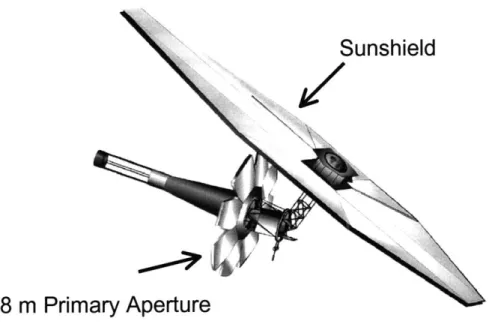
Sunshield
8 m Primary Aperture
Figure 1.3 Next Generation Space Telescope -GSFC Designa a. http://www.ngst.nasa.gov
1. http://www.ngst.nasa.gov
Background 23
Angular resolution refers to the size of the smallest discernible detail of an image. It is often given in terms of the angle that an object subtends rather than the actual size of the object. A penny at seven feet away from your eye subtends approximately the same angle, half a degree, as the moon in the night sky. The penny 24 miles away subtends an angle of
0.1 arc-seconds, which is the resolution of HST. The angular resolution of a telescope is
proportional to the aperture area and inversely proportional to the wavelength of light. Therefore, for a fixed aperture size, resolution is higher at shorter wavelengths, and for a fixed wavelength, resolution improves as the aperture increases. Since NGST is intended to observe at longer wavelengths than HST, its aperture area must be larger to achieve the same angular resolution as HST.
NGST's primary mirror is 8 meters in diameter, almost four times the size that of HST. However, a solid 8m diameter mirror cannot fit into any existing launch vehicle fairings and it would be extremely heavy and costly to launch. One solution to these constraints is a deployable, light-weight 8m diameter mirror. Therefore, the primary mirror used for
NGST must be deployable.
Another requirement of designing an infrared telescope to detect faint objects is that the thermal background (heat) must be smaller than the signal it is trying to detect. For NGST to reach its designed operating temperature of 35 degrees Kelvin, it must be removed from large sources of heat. The first source, Earth and the heat of the sun reflected off of Earth, is reduced by launching the satellite far from Earth at the L2 libration point. Once in orbit, the sun is the primary source of heat impinging on the telescope. To shield the optics from the heat, a large sunshield, approximately the size of a tennis court is required.' (Figure 1.3) The sunshield adds a large flexible appendage to the spacecraft that adds low frequency modes to the telescope dynamics.
24 INTRODUCTION
Space Interferometry Mission
The Space Interferometry Mission (SIM) planned for launch in 2006, is the first space-based interferometer. Its goals are to perform precision astrometry and demonstrate inter-ferometry technology for future missions, such as TPF. Interferometers combine light from multiple apertures and create a single image with higher resolution than either aper-ture could produce alone. The angular resolution of the interferometer is determined by the distance between the apertures, rather than by the individual aperture size. Therefore, interferometers provide increased angular resolution without significant increase in mirror
mass, cost, and size [DeYoung, 1998].
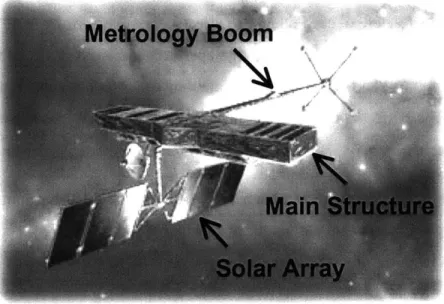
SIM, shown in Figure 1.4, is a 10m baseline Michelson interferometer. The baseline is the distance between the two apertures perpendicular to the incoming science light. SIM will be able to measure the angular position of stars to an accuracy of 4 microarcseconds, which is several hundred times more accurate than any previous telescope. The resolution provided by SIM will result in improved planet detection, with the ability to detect smaller planets closer to its parent star.
The main structure in Figure 1.4 is a lightweight, flexible truss that supports the light-col-lecting apertures. The metrology boom and the solar panels are also flexible structures. The optics on SIM are meters apart, yet their relative positions must be controlled to sub-nanometer level precision in order for the interferometer to achieve its astrometry goals.
1.1.2 Space Telescope Stringent Performances
Both NGST and SIM share a common goal of improved angular resolution. However, although the trend for improving telescope performance is towards larger aperture tele-scopes, the design solution of merely increasing the mirror size is limited by existent astronautical technology. The aperture size must be increased by innovative methods such as those mentioned for NGST and SIM: lightweight optics and interferometry. The chal-lenge associated with these designs is the reduction of structural rigidity compared to designs like HST. Lightweight materials are less stiff than glass and subject to
deforma-Background 25
Figure 1.4 Space Interferometry Mission
tion and vibrations. Deployable truss structures are also more flexible and add low fre-quency modes to the system. These effects must be taken into consideration when designing the telescope, to ensure that the vibrations attenuated by the structural flexibili-ties can be adequately damped or isolated from the optical components.
The optics demand extremely quiet, vibration-free environments. The surface of each mir-ror must hold its shape to fractions of the wavelength of the science light in order to reduce wavefront error. The wavefront consists of light that left the science target at the same time. Because the star is much further away than the dimensions of the telescope, the wavefront entering the telescope is considered planar; however, as it bounces off one mir-ror to the next, if the surface of the mirmir-ror is not a perfect ellipsoid, each ray of light will travel a slightly different distance than its neighbor. Thus, the wavefront will deviate from a perfect plane. For glass mirrors, the surface can be polished and manufactured to be as smooth as required. For example, the largest deviation of the surface of the Chandra X-ray telescope mirrors, the smoothest mirrors ever produced, is within several atoms.1 If, to
26 INTRODUCTION
reduce weight, the telescope mirror is not made out of glass, but a flexible membrane, then the shape must be maintained by means other than structural rigidity.
Motion of mirrors relative to each other also affects telescope performance. In an interfer-ometer, the light gathered from two separate apertures must travel the same distance, or optical path length (OPL) from collectors to combiner to interfere constructively and cre-ate an image. Therefore the maximum optical path difference (OPD) allowable is on the order of nanometers.
A telescope with high angular resolution has failed in its mission if it cannot be steadied to look at the target for an adequate length of time for the camera to collect enough light. This deviation from the intended target direction represents the ability of a telescope to stay pointed on its target. Wavefront error, OPD, and pointing are a few possible optical performance metrics.
These optics are mounted to a structure whose purpose is to hold them in the correct figuration as well as support the other subsystems of the spacecraft bus. Again, con-strained by mass, cost and launch volume, this structure cannot be as rigid as its ground based counterparts are. Engineers must look for alternative structural designs, whose trend is toward lighter and deployable structures, with the optics, themselves, following the same trend. These light, flexible structures easily transmit vibrational noise, which intro-duce errors into the optics train and reintro-duce the quality of the image. The solution is either to isolate the optics from the sources of noise and/or to add controllers that will actively eliminate the vibrations to a level that is acceptable for optics performance.
These structural flexibilities are not a problem for the telescope unless a disturbance excites them. When satellites are placed in low earth orbits, they encounter atmospheric drag, gravity gradient or magnetic torques that may move the satellite from its desired atti-tude. Further from earth, in geosynchronous orbits or beyond, the effects of solar wind are
Integrated Modeling 27
predominant and can cause external torquing on the satellite to move it from its desired attitude. To compensate for such disturbances from the orbital environment, reaction wheels are used for attitude control. However, reaction wheels themselves are a source of mechanical disturbances on board the telescope. If the wheel's center of gravity or primary inertial axis is off the axis of rotation, the resulting imbalances cause the vibrations that impact disturbances to the system. Reaction wheels are the largest expected disturbance source on space telescopes. Other possible on board disturbance sources are cryocoolers, guide star sensor noise, digital to analog quantization noise, and solar thermal flux.
1.2 Integrated Modeling
Integrated modeling is a methodology that combines the models from different sub-disci-plines into one complete input-output system. It is interdisciplinary in nature, but in this thesis, the term will refer to the modeling of high-performance opto-structural plants, which includes the disciplines of structural dynamics, optics, and controls. The precision controlled opto-structural plant captures the essential characteristics of different space telescopes and standardizes the analysis [Basdogan, 1999, Gutierrez, 1999, Melody, 1995, Mosier, 1998a, Robertson, 1997]. Figure 1.5 is an example of an integrated model sche-matic. The highlighted portion within the dotted lines is the integrated model. The input is unit intensity white noise, d, and the outputs are the performances metrics, z. The blocks within the shaded region are the individual components of the integrated model. The fol-lowing description of the integrated modeling is based on the work of Homero Gutierrez.
The "Opto-Structural Plant" block in Figure 1.5 represents the structural model of SIM. The model is built using finite element methods and represented in state-space format. The structural model represents the dynamics of the system, and accepts forces, f, as input and outputs the states, x, of the system as shown in Figure 1.6.
Performance metrics are use to determine if the telescope meets the engineering require-ments, thereby accomplishing its science objectives. Two examples of performances are shown in Figure 1.5: OPD and pointing. The OPD metric is shown as the RMS of the time
28 INTRODUCTION
White Noise Input
Appended LTI System Dynamics Opto-Structural Plant
SIM V2.2 2184 states Optical
Control
Process Noise
Phasing (OPD)
az1
=RMS
OPDFigure 1.5 Example Integrated Model: SIM
---A > Ad,Bd,
W
4
F7
Cd,Dd W -
plant
XC
U controller
y
AeBCCCDC
Integrated Modeling 29
history. The pointing error, or wavefront tilt (WFT) is given by the root sum squared (rss) of the radius of the time history. The pointing time history information is shown projected on the plane of the telescope's receiver.
The performance block, Cz, is not shown in Figure 1.5 because it is modeled in the plant model. The state-space matrix that is represents linearly combines the system states, x, to produce the output metric(s), z. Calculating space telescopes performance metrics requires creating a sensitivity matrix from the plant states to the performance metrics. Calculating these sensitivities require structural engineers and optical engineers to fuse their models
together.
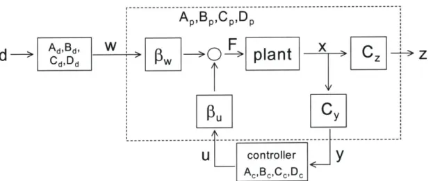
In Figure 1.6, w is the disturbance force and the block, $w, represents the state-space matrix that maps the disturbances onto the appropriate degrees of freedom in the structural model. This block is also not shown in Figure 1.5, because it, too, is contained within the plant model.
The disturbances can be input into the structural model as a white noise shaping filter. The disturbance filter has its own states and state-space representation as shown in Figure 1.6, where d is the white noise input and w is the shaped disturbances. Modeling the distur-bances involves either determining the time histories or creating the state-space filter or both. The subscripts d and p denote the disturbance verses the plant state space matrices, respectively.
If the plant does not meet the performance requirements in the presence of disturbances, a
controller may be used to improve the system performance. In Figure 1.6, output y is input to the controller and the controller output, u, drives the plant. All blocks except the con-troller are part of the plant's state space representation as indicated by the dotted line. The complete integrated model has the state-space formulation of the plant dynamics,
30 INTRODUCTION
1.3 Thesis Objective
1.3.1 Importance of Accurate Structural Models
Section 1.1.1 and Section 1.1.2 introduced the difficulty of designing space telescopes to achieve the science goals of the Origins Program. The term nanodynamics appropriately implies the degree of precision to which the structures must be controlled.
The fundamental reason why analytical models are used to predict the capabilities of the design is because some structures can not be built for testing; also, the environment the system is being designed for cannot be adequately reproduced [Moses, 1998]. At the con-ceptual design stage, multiple architectures are compared to determine the direction for future development. Once an architecture is chosen, a number of design iterations are per-formed before the actual spacecraft is built and deployed. The performance must be able to be predicted through structural analysis to assess the design without building the struc-ture at each iteration. Analytical modeling provides major cost and time savings by doing as much analysis on computers as possible instead of experimentally.
Besides time and cost savings, some telescopes are impractical to build for ground testing. NGST's sunshield, approximately the size of a tennis court, is an example of the trend in future designs towards increasingly larger spacecraft. Though individual subsystem proto-types are built for testing, the size of the complete spacecraft limits the practicality of inte-grating the entire structure on the ground. Space structures are also designed for operation in a zero-g environment, and may not be able to support their own weight on the ground. Without ground test verification, the analytical model must accurately capture the
dynamic behavior of the structure in order to have confidence in the performance predic-tions. Early in the project, however, the design is not fully complete when analysis starts and key design decisions are made. It is important to know what information from the low fidelity models can be used to make these critical decisions.
Thesis Objective 31
1.3.2 Model Fidelity
The accuracy of a model can only be as good as the maturity of the design it is based upon. The maturity of the design refers to how well the iteration represents the final version. If the iteration is in the conceptual design stage, analysis will not accurately reflect the char-acteristics of the finished product. If the iteration is near final, then its model will still not reflect the actual behavior of the "true" system, but will have less error than the low itera-tion model and the dynamics will more closely resemble the actual behavior of the final system. If the iterations are complete and the structure is being built or is built, then its model will represent the behavior of the system only to the uncertainty that is within the model itself and not due to uncertainties in the design [Berman, 1999]. Hence, as the design iterates and stabilizes towards the final solution, the fidelity of the model improves and becomes more reliable for predicting performance. In studying model fidelity, it is important to understand how the behavior of low fidelity models resemble the truth model. Low fidelity designs occur at the beginning of the design process, when a mission concept and architecture are chosen. The design requirements are determined based on a flow down from the science requirements. For example, a maximum OPD RMS determined necessary for mission success is used to determine the extent that the structure must be made rigid, isolated, or controlled. At this stage, only a basic overview of the structure is known with general dimensions in order to keep the optics it its nominal positions.
From the different possible architectures to satisfy the requirements, one approach is cho-sen that satisfies the cost, requirements and constraints. As the design progresses, more subsystem requirements are determined, dimensions of components and materials are cho-sen, and a more detailed layout of the structure is created. Fidelity increases further in the design process when the design becomes fixed and most dimensions and material proper-ties are known.
To understand the errors associated with model fidelity, an analogy can be made between the model evolution of a design in progress and the model updating evolution of an
exist-32 INTRODUCTION
ing structure. This analogy is helpful because model updating is a well-researched topic; there is ample material on the errors associated with fidelity error of the model of a single design iteration [Berman, 1999]. Joshi et al. discuss model fidelity in the sense of model updating, where the increasing fidelity models are the increasingly accurate models of the same built structure [Joshi, 1997].
The updating process begins with a model based on simplifying assumptions and nominal material properties gathered from look-up tables. The model improves as the assumptions are checked for accurate representation of the structure's behavior and as parameter values are tested [Glease, 1994]. The model evolution of the design in progress undergoes a sim-ilar process, assuming that the models compared at each iteration have been updated. These models are based on a design that has simplifying assumptions and lack of parame-ter value knowledge. As the design evolves, the assumptions are solidified and the param-eter choices are made. Thus there is a local model evolution within model updating and a global model fidelity evolution as a structure is being designed, as illustrated by Figure 1.7.
This analogy can help explain the types of errors involved in model fidelity evolution. As the term "evolution" implies, there is a change in the type of errors associated with the model at the different design stages. In the earlier stages, non-parametric errors predomi-nate. These are errors that cannot be associated by a parameter (mass or stiffness) of a model element, but are akin to a "lack" of a parameter. Early design errors are associated with errors in design assumptions.
In early design stages and for initial models, large structures can be modeled by a simpler element, such as representing a truss by a beam element. This simplified model, called a stick model, saves computational time when conducting analysis. The beam's dynamics will resemble the global, fundamental characteristics of the truss while not requiring as many elements. The beam will not adequately resemble all the characteristics of the truss, but because the parameters, configuration and dimensions are not fixed, the uncertainty in
~~U..,.. Thesis Objective 33 Model Fidelity Evolution A A D v 0 Design Evolution I I I I > st Iteration 2nd 3rd Flight
Structural Design Accuracy
Figure 1.7 Model Fidelity Evolutionthe design is on the same order of magnitude or larger than that associated with the
inaccu-racies of the stick model.
(D Nominal Solution
Error Budirse nt
Error Bounds
A
D
1 2 3 4
Design Iteration >
Figure 1.8 Uncertainty [Gutierrez, 1999]
i 0 0 0 C Initial Final Model Updated Model
A Actual Progression of Model
t
Decoupled Model ProgressionC) C CE t2 (D a.
34 INTRODUCTION
Figure 1.8 illustrates the performance prediction and error bounds for four design itera-tions of an imaginary system. The vertical scale in Figure 1.7 can be paralleled with the error bounds of Figure 1.8, where as the error bounds decrease, the analytical model accu-racy increases. For Design 1, the performance prediction does not meet the requirement. For Design 2, the design is improved until the nominal solution meets the requirements, but the addition of the error bars shows that the design may or may not meet the require-ment. Designs 3 and 4 are two different approaches from Design 2. Design 3 improves the design so that with the uncertainty, the design will meet the requirements. Design 4 does not change the design, but reduces the uncertainty.
Thus there are two ways that the error bars can be defined. The first is with accurate mod-eling but a low iteration design and the second is with a finalized design but a poor analyt-ical model. Both of these types of error sources can contribute to poor model fidelity. The objective of this thesis is to look at model fidelity evolution compared to model updating to understand how the behavior of low fidelity models resembles the truth model.
1.4 Dynamics Optics Controls Structures (DOCS)
The Space Systems Laboratory at MIT has developed a set of software modules and a design and analysis methodology for precision space telescopes called DOCS. DOCS stands for Dynamics Optics Controls Structures and a flowchart for the methodology is shown in Figure 1.9.
The first step in DOCS is modeling all the components of the integrated model. Starting with the design of a telescope, the structure and optics models are created and the bance sources are determined and modeled. Since reaction wheels are the primary distur-bance source for space telescopes, a lot of work has been done to model their disturdistur-bances.
Work on reaction wheel modeling has been done by Rebecca Masterson
Dynamics Optics Controls Structures (DOCS)
Inputs 111 Software Modules |1 | Outputs Figure 1.9 DOCS Flowchart
The individual models are then assembled in the next stage of DOCS. Before being ana-lyzed, however, the model must be updated, conditioned and reduced. The necessity of conditioning is a by-product of using computers to analyze structures. Poor numerical conditioning can cause problems in the analysis not related to the inherent design. For example, if the units of the structure's dimensions are in meters and the performance met-rics are in nanometers, the model will be handling two sets of numbers nine orders of mag-nitude apart. Additionally, the final model can have an extremely large number of degrees of freedom with the addition of the dof's of the disturbance model and the controller. When converted to modal coordinates, not all modes are observable or controllable, and are unnecessary additional information adding to computational expense. Work on condi-tioning and model reduction has been done by Scott Uebelheart [Uebelhart, 2001].
After preparing the model, it then moves to the next stage, analysis. The fundamental anal-ysis that is done is the disturbance analanal-ysis, which will determine if the model will meet
36 INTRODUCTION
the performance. The disturbance analysis methods used in the Space Systems Lab and in this thesis were developed by Homero Gutierrez [Gutierrez, 1999]. Disturbance analysis can be done open or closed loop. If the model does not satisfy the performance require-ments open loop, then a controller is added to the system. Greg Mallory did work on con-troller tuning for space telescopes based on measurement models [Mallory, 2000a]. Mathematical models of real systems inherently have errors associated with them because the models contain assumptions and simplifications in order to be made. While the distur-bance analysis may predict that the model meets the performance requirements, the uncer-tainty analysis determines the error bounds about this prediction [Bourgault, 2000]. After completing the analysis, the results are studied in the design stage. If the model does not meet the performance requirements, then a change in the controller and/or a change in the telescope design must be made. Sensitivity analysis determines how the changes in parameters affect the performance of the system. If the model does meet the performance requirements, design of the system is not necessarily over. An isoperformance analysis finds multiple sets of design parameters that result in the same performance. This analysis can be important during manufacturing considerations; as some subsystems, like reaction wheels or optical sensors, do not have a continuous array of sizes or quality to choose from parameters traded. Also, improving the performance of one subsystem may be less expensive than improving the performance of another. Work on isoperformance is being done by Olivier de Weck [DeWeck, 1999].
1.5 Thesis Overview
Figure 1.10 illustrates how the organization of the chapters in this thesis fits in with the model fidelity evolution diagram of Figure 1.7. First, in Chapter 2 a two-dimensional truss structure is used as an example problem that demonstrates the evolution of a low fidelity "stick" model to a high fidelity "truth" model. Then, in Chapter 3, the Origins Testbed is given as an example of a high fidelity design -a structure that has already been built. The analytical model updating of the testbed is used as a demonstration of the model updating
-- EU - I
Thesis Overview 37
Model Fidelity Evolution Sample Problem Chapter 2 Low Fidelity Disturbance Analys ARGOS Testbed Chapter 4 is A High Fidelity Model Updating Origins Testbed Chapter 3 I | | >I Concept Flight
Figure 1.10 Thesis Roadmap
error analogy to design evolution. In Chapter 4, the ARGOS testbed is described as an example of a low fidelity model. A disturbance analysis is done on ARGOS and
conclu-sions on the analysis are drawn based upon knowledge of ARGOS' model fidelity.
Design
Chapter 2
SAMPLE PROBLEM
In this chapter, a truss sample problem is presented to describe the different stages of model fidelity. The design maturity is simulated by different finite element types: (listed in order of increasing fidelity) a Bernoulli-Euler beam, a Timoshenko beam, a truss with rod elements and a truss with bending beam elements. Model updating is simulated by mesh-ing the finite elements at different degrees of refinement. The models are compared to a
"truth" model, which is the highly refined truss with bending elements.
2.1 State Space Representation
In this section the state space representation of equations of motion in structural modal form is derived. Then the disturbance states are appended to the plant states to create the integrated model. State space representation is first introduced using a simple harmonic oscillator as an example, and is then applied to a discrete multi-degree of freedom system. The 1-dof harmonic oscillator is shown in Figure 2.1, where m is the mass, k is the spring constant, c is the damping coefficient, x is the displacement of the mass and F is the force
applied to the mass.
The equation of motion for the mass is given by:
mx+cx+kx = F (2.1)
Then solving for the acceleration of the mass gives:
40 SAMPLE PROBLEM
X
Figure 2.1 Simple system
-- _c) -(_k F+
x= -I x )+ + (2.2)
Two new variables xi and x2 are defined such that: xI x
(2.3) x2 X
Written in matrix form, the equation for the time derivatives of the new variables, x1 and
x2, using equations (2.2) and (2.3) are:
- 0 1
-0
1] = [0 c + F (2.4)
X2 - -- X2 ~
The vector, [xI, x2]T, contains the states of the system. Equation (2.4) is helpful for visual-izing the state space representation since it still retains the physical characteristics of the system. The derivation of the structural modal form for the multi-degree of freedom sys-tems is based on the physics of the structure, but the resulting equations are in modal coor-dinates, which are less physically intuitive. Notice from equation (2.4) that the number of
State Space Representation 41
states is twice the number of degrees of freedom of the system. This fact always holds when converting to a physically-based state-space representation.
For discrete systems with more than one degree of freedom, the mass and stiffness terms are matrices instead of scalars. The equations of motion of a conservative (undamped), linear, time invariant (LTI) system can be written as:
Mx+Kx = F (2.5)
where M and K are the (n x n) mass and stiffness matrices, respectively, x is a vector of the n degrees of freedom (DOF) in the physical coordinate system, and F is a vector of external forces acting on the system.
Assuming that the homogenous solution of equation (2.5) is of the form:
X = $ewt (2.6)
and substituting this solution into equation (2.5) while setting F = 0, we obtain:
-W2M$+K$ = 0 (2.7)
Then, by substituting w2= X and rearranging, we obtain the generalized eigenvalue prob-lem:
(K-XAM)$5 = 0 (2.8)
where X; is the ith eigenvalue and $j is the corresponding eigenvector. The index, i, ranges from i = 1...m, where m is the number of modes of the system, (m 5 n). In general, the total number of modes is equal to the number of DOF, but it is not always necessary to include all modes in the model. For instance, when using finite element methods, the higher modes are often neglected. They inherently have high error due to the linearization of finite elements and they add to the computational expense for large models. Addition-ally, if the analytical model is compared to data, the higher modes may exceed the fre-quency of the data and are then unnecessary information.
42 SAMPLE PROBLEM
Due to the orthogonality of the eigenvectors, the following relationships hold:
0OT 0 0 TM ( = I
0
[D
j
(2.9)where (D is the (n x m) eigenvector matrix. The superscript, 0, indicates that 0D is mass normalized. The columns of 0i) are the eigenvectors $1, 0,
#03,--,
Om, I is the identity matrix, and L22 is a diagonal matrix whose elements are the eigenvalues Xi = 012, X2 =(022, X3 32 Xm m2.
Using equation (2.9), equation (2.5) can be decoupled through a coordinate transformation from physical to modal coordinates. Substituting:
x = 0 ( (2.10)
into the equation of motion we obtain:
M 0(+ K** D = F (2.11)
where is the vector of modal coordinates. Pre-multiplying equation (2.11) by cD gives:
0 D T M0 )+0DT K = Oi F (2.12)
Then using equations (2.9) and (2.11), we rewrite equation (2.12) as:
+A2 =
Q
(2.13)At this stage we add damping back to the system by assuming that the damping is propor-tional to the modes. This assumption is valid for lightly damped systems:
(2.14)
State Space Representation 43
where Z is the diagonal matrix of damping coefficients.
The forcing term is partitioned into two components: forces from disturbances, F, and forces from control actuators, Fu:
Q
= 0DTF
= 0DT Fu+ 0) F, = 04 Tpuu+0Tp) w (2.15)where the (n x nu) matrix,
@u,
and (n x n,) matrix, P, map the actuator forces and dis-turbances, respectively, onto the correct degrees of freedom, nu are the number of actuator inputs and nw are the number of disturbance inputs. The 0DT matrix completes the coordi-nate transformation so that the actuator forces and disturbances act on the correct modal coordinates. Substituting into equation (2.14) and rearranging we have:= - 2ZOQ 22+ 0 ) $w wpuuT+ (2.16)
Equation (2.16) is the equation of motion in the modal coordinate system. It is rearranged as a system of equations and written in matrix form by defining a new state variable:
qp -(2.17)
Then the equations of motion in state-space form are:
0 I 0 0
-[Q2
-2Z92]q
+[
BU
0TB]
(2.18) A(2mx2m) BU (2mx>n) B, (2mxn )
where A is the plant dynamics matrix, m is the number of modes retained Bu is the plant actuation input matrix, nu is the number of controller inputs, Bw is the plant disturbance input matrix, nw is the number of disturbance inputs.
Equation (2.18) is written in the structural-modal form. This form is most useful when the mass and stiffness matrices are unknown, but the eigenvalues and eigenvectors are known.
44 SAMPLE PROBLEM
To complete the state space representation, the output is written as a combination of the state variables:
y = Cx+Dyuu+DY~w (2.19)
where C maps the correct degrees of freedom to the output. To transform to modal coordi-nates, x = 0CD is substituted in equation (2.19). To rewrite equation (2.19) in matrix form, and are factored out and replaced by qp to obtain:
y= CY@ C,"o+ [D.] u+ [Dw] w
- ,r-'(2.20)
C (n xr D,(nym> D (nym>
where Cy is the plant output matrix and ny is the number of outputs. The matrices Dyu and Dy, are the feedthrough matrices from the control forces and disturbances, respectively, to the output and are usually zero.
Similarly, the performance can be written:
z=[C
_C
"O
]
+
[D
]u+ [D
w
q J D-nz-xy D~(2.21)
C(nz>am)
Du("zmu> D (n 4>nwhere Cz is the performance matrix, and nz is the number of performances. The matrices Dzu and Dzw are the feedthrough matrices from the control forces and disturbances, respectively, to the performance and are usually zero. The difference between y and z is that the outputs, y, are the sensor measurements used by controllers for calculating actua-tor control signals and the performances, z, are the metrics used to determine if the plant is meeting requirements.
State Space Representation 45
qP = Apqp + Bau + Bw
y = CYq,+ Dyuu+ DYw (2.22)
z = Czqp+Dzuu+ Dzww
A state-space model can be derived through an analytical model of the M and K matrices. If the structure being modeled has already been built, then the analytical model can be compared to the experimental data. Noise is input at the correct location and data are taken from sensors at the output nodes. A set of A,B,C,D matrices is then found that best fits the system ID transfer function. This model is called the measurement model and is assumed to be a more accurate representation of the plant dynamics than the analytical model [Marco-Gomez,1999]. Unfortunately, the measurement model is not created based on relationships among physical parameters and, therefore, must be recalculated anytime the structure or environmental conditions change.
Disturbance states:
As described in Section 1.2, disturbance can be modeled as a state space filter through which unit intensity white noise is shaped to produce a Power Spectral Density (PSD) with the equivalent energy and frequency content as the actual PSD of the disturbance. The disturbance represented in state space form is denoted by a subscript d:
qd = Adq + Bdd (2.23)
w = Cdqd
where qd are the disturbance states, d is the white noise input, and w is the shaped distur-bance output.
A new state vector is created by appending the disturbance states to the plant states:
46 SAMPLE PROBLEM
and the system equations are:
q = A 0 + Bd d
LBWCd A pj
[ Oj
(2.25)Z =[0 Cj q +
[0]
dwhere d is the white noise input and z is the performance output.
2.2 Problem Formulation
A simple truss is used as a sample problem to illustrate the evolution of model fidelity, which is the increase in the accuracy of the model as the design iterates to the true system. The initial design is a simple beam and the final design is a beam-like truss. To adequately compare the low fidelity beam-type model with the high fidelity truss model, the beam is forced to have properties equivalent to the final truss design. In an actual design scenario, where the final design is not known a priori, the initial design will include parametric errors in addition to the non-parametric errors discussed in this section.
In this example, model fidelity evolution is demonstrated through the use of different finite elements and by refinement of the finite element mesh. The truss is first represented as a stick model with Bernoulli-Euler beam elements and then with Timoshenko beam ele-ments. The next step in the model evolution is to accurately model the truss geometry. However, the truss is first modeled using rod members which only have forces and dis-placements in each member's axial direction. Finally, the members are modeled as bend-ing members. A highly refined model of the truss with bendbend-ing members is considered the "truth" model against which to compare the others.
The type of finite element determines the modes that are modeled. The stick models only capture the global modes of the truss and not the effects of the flexibility of the individual truss members. Because the truss has a low aspect ratio (length/depth) the Timoshenko beam captures the truss' global bending modes at a significantly higher accuracy than the
Problem Formulation 47
Bernoulli-Euler beam. A truss modeled with rods does not capture the local bending modes of the members, but captures the stiffness characteristics of the truss more accu-rately than the beam elements. Finite element mesh refinement increases the number of modes calculated and allows the lower-frequency modes to converge to the continuous solution.
The truss consists of eight square bays with alternating diagonals across each face. It is fixed at one end, x = 0, and free at the other, x = L. The members of the truss are circular beams of radius r. The horizontal and vertical members have length (Lm = L/8) and the diagonal members have length A2 Lm. The nodes are labeled across the top from left to right then across the bottom from left to right. A downward force is applied to the top of the truss at node 6, and the performance is the truss tip displacement as shown in Figure 2.2. The truss configuration and property values resemble one face of the three dimensional truss tower of the Origins Testbed. However the total length was fixed to Im for numerical simplicity. The property values are listed in Table 2.1.
LM Force Displacement
c
MI
L
Figure 2.2 Example problem truss schematic
2.2.1 Equivalent Inertia
An advantage of modeling a truss with a stick model is the reduction of the number of degrees of freedom and thus the reduction of the size of the model and computational time. However, to accurately represent the truss as a beam, the stick model must have sim-ilar fundamental characteristics, such as static deflection (static simsim-ilarity) and/or
funda-48 SAMPLE PROBLEM
TABLE 2.1 Truss property values
Variable value material AL E 7.2E-10 Pa v 0.33 p 2800 kg/m3 L I m Lm 0.125 m r 0.004 m
mental mode(s) (dynamic similarity). A simple analysis of the truss is deformed to determine the equivalent beam properties. Then the beam is used for analysis of the larger
system.
Sun et al. present a method to find the equivalent properties for a truss [Sun, 1981]. The authors solve for the three equivalent beam stiffnesses: e.g. axial stiffness (EA), bending stiffness (EI), and shear stiffness (GA) assuming that these properties are decoupled. Necib et al. discusses how to calculate the entire matrix of coupled stiffnesses as well, which is important for asymmetrical structures [Necib, 1989]. The decoupled stiffnesses will be used for the sample problem. The equivalent inertia properties of the truss are the mass per unit length (pA) and the rotary inertia per unit length (pI) and their calculations are also presented by Sun et al.
Because equivalent beam properties are calculated via static deflections of the truss, the following derivation is for a simple, static truss using ideal truss assumptions: members experience only compression and tension [Strang, 1986]. Each node has two degrees of freedom as shown in Figure 2.3. There are eighteen nodes and 33 members.
The vector, x, is a vector of unknown displacements at each node, where superscripts H and V specify horizontal and vertical displacement, respectively: