Publisher’s version / Version de l'éditeur:
Vous avez des questions? Nous pouvons vous aider. Pour communiquer directement avec un auteur, consultez la
première page de la revue dans laquelle son article a été publié afin de trouver ses coordonnées. Si vous n’arrivez
Questions? Contact the NRC Publications Archive team at
PublicationsArchive-ArchivesPublications@nrc-cnrc.gc.ca. If you wish to email the authors directly, please see the first page of the publication for their contact information.
https://publications-cnrc.canada.ca/fra/droits
L’accès à ce site Web et l’utilisation de son contenu sont assujettis aux conditions présentées dans le site LISEZ CES CONDITIONS ATTENTIVEMENT AVANT D’UTILISER CE SITE WEB.
The 27th American Towing Tank Conference [Proceedings], 2004
READ THESE TERMS AND CONDITIONS CAREFULLY BEFORE USING THIS WEBSITE. https://nrc-publications.canada.ca/eng/copyright
NRC Publications Archive Record / Notice des Archives des publications du CNRC :
https://nrc-publications.canada.ca/eng/view/object/?id=b9d45f26-f67e-42fc-b367-ef85776e9836 https://publications-cnrc.canada.ca/fra/voir/objet/?id=b9d45f26-f67e-42fc-b367-ef85776e9836
NRC Publications Archive
Archives des publications du CNRC
This publication could be one of several versions: author’s original, accepted manuscript or the publisher’s version. / La version de cette publication peut être l’une des suivantes : la version prépublication de l’auteur, la version acceptée du manuscrit ou la version de l’éditeur.
Access and use of this website and the material on it are subject to the Terms and Conditions set forth at
An advanced model autopilot control system
An Advanced Model Autopilot Control System
J. Millan, G. Janes, E. Kennedy, D. Cumming
Institute for Ocean Technology
National Research Council
St.John’s, Newfoundland, Canada
Abstract
Advancements in instrumentation and control systems for model test-ing are often driven by new and sometimes very demandtest-ing test pro-gram requirements. Ever-improving wireless communications, miniatur-ized power electronics and computer systems and software have made it possible to achieve control and instrumentation objectives that were not practical in model test programs of a decade ago. This paper describes a model autopilot system that was developed last year at the Institute for Ocean Technology, having significant advantages over earlier systems. The autopilot and the heading sensor are not on the model, allowing very small model vessels with low power consumption to be controlled. The system also incorporates a Kalman filter to provide smooth position updates and a reduction of first-order wave disturbance in the rudder command signal.
1
Introduction
In 2000, the Institute for Ocean Technology (IOT) identified a requirement for a new model autopilot that could function with free-running vessels in the off-shore engineering basin (OEB). Utilizing software and techniques that had been recently developed for IOT’s dynamic positioning (DP) system in combination with existing remote control (RC) hardware and software, an autopilot system was developed. This first autopilot was based on two full-sized industrial PCs which seriously handicapped the utility of the design due to the high power con-sumption. Heading feedback was from an on-board spinning-mass gyroscope. It was clear from the operational experience with this system that a smaller au-topilot with lower power consumption was needed. Additionally, it was desired that the new autopilot should utilize an alternative sensor to the gyros, which are difficult to maintain and troublesome to operate. An effort was undertaken during 2002-2003 to implement an advanced autopilot that would rectify many of the shortcomings of the first system. This new system was able to draw on hardware and software that had recently been developed for other model test programs. This resulting autopilot met most of the design expectations and performed extremely well during a set of free-running seakeeping experiments on a 1:12 scale free-running model during the spring of 2003 (see figure 1).
Figure 1: A model equipped with the newly developed autopilot in the IOT offshore engineering basin in April 2003.
2
System Architecture
In order to improve on the older autopilot, the following key features had to be considered:
• Light Weight: reduce equipment mass for smaller scale vessel testing • Low Power Consumption: reduced power consumption extends battery
life (and hence operational time) and allows for lower battery weight • Reliable Feedback: heading feedback must come from a reliable source These requirements could be addressed by removing much of the autopilot function from the model boat. In the early autopilots, the feedback sensor (the gyro) and the autopilot computer were both located in the model (figure 2).
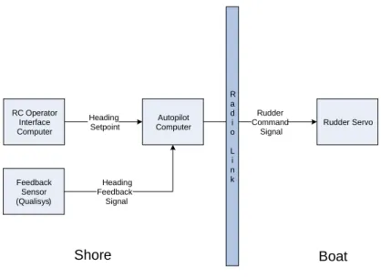
The general concept for the new design was to take this function out of the boat and place it on the shore to reduce the weight and power requirements, pictured in figure 3. The gyro has been replaced by the Qualisys shore-based optical tracking system. The advantages of this approach are the requirement only for a one-way radio link and a reduction of equipment (and thus power consumption and mass) to be placed in the boat. Due to these obvious advan-tages it was decided to take this approach for the autopilot design. The main risk to this approach is that the full-basin optical tracking system used in the tank has some limitations that could present a significant challenge to real-time control.
Autopilot Computer Feedback Sensor (Gyro) RC Operator Interface Computer Rudder Servo Heading Setpoint Rudder Command Signal R a d i o L i n k Boat Shore Heading Feedback
Figure 2: Block Diagram for early autopilot
Autopilot Computer Feedback Sensor (Qualisys) RC Operator Interface Computer Rudder Servo Heading Setpoint Rudder Command Signal Boat Shore R a d i o L i n k Heading Feedback Signal
3
Optical Tracking and Control
For reliable closed-loop control (as in an autopilot), the control system must be supplied with reliable, error-free heading information supplied in real time (at a constant update rate). This is due to the fact that the response of the rudder, and hence the vessel, is directly related to the feedback signal in a closed-loop control system.
The optical tracking system (a Qualisys system) in the OEB consists of a pair of digital video cameras and processing systems with a wide field of view. They view most of the tank, so they are able to track a set of active infrared targets on the model vessel. From each frame grab (25Hz frame rate), the system determines the attitude and position of the vessel in a tank global coordinate frame, based on the position of the visible targets A typical tracking signal for a vessel in the tank will have some drop-outs (due to missing targets) and errors (due to false targets). We can refer to these generically as "glitches". The system identifies both types of errors by flagging them with an unfavourable error rating in the RMS channel. The autopilot clearly needs some way of identifying the glitches in real time and for filling in the lost data so that a reasonable rudder command can be calculated. A number of alternatives were considered, including the following:
• Low pass digital filter: since most of the Qualisys signal issues are glitches, they could be filtered using a low pass filter with the appropriate settings. • Track and Hold: when the signal is "good", it is passed through (tracked) and when it is "bad" (unreliable, or containing errors), it is held at the last known good value.
• Kalman filter: given a dynamic model of the vessel, a Kalman filter can be used to remove sensor noise and provide a prediction of the heading signal at each time step of the autopilot update cycle.
In order to assess the effectiveness of these methods, each was coded in Matlab and tested offline using: 1) actual Qualisys tracking data from previous tests and 2) simulated data. Based on the results of these simulations, it was decided that the Kalman filter was the best option.
4
Kalman Filter
The Kalman filter is useful for removing stochastic sensor noise with a constant covariance characteristic. Unfortunately, the noise content of the optical track-ing 6DOF data is not easily modeled, since the covariance is dependent upon the location of the vessel with respect to the cameras, the lighting level, and even the sea state in the model basin. In addition, the drop-outs and glitches are not predictable by a linear stochastic model such as that embodied in the filter. The primary utility of the Kalman filter in our application is as a pre-dictor, (or gap-filler) since it can be used to generate a model-based prediction
of the heading, even in the absence of a measurement, and for unevenly spaced data points.
In order to implement the Kalman filter, a simple linear (and preferably time invariant) model is required. The first-order Nomoto steering model relates the rudder angle to the heading angle, characterizing the steering of a vessel with two parameters, K and T, that vary as a function of forward speed. For a fixed forward speed, the Nomoto steering dynamics are given by the following equation:
T ¨ψ + ˙ψ = Kδ (1)
where δ is the rudder angle and ˙ψ and ¨ψ are the heading angular rate and acceleration respectively. This model provides a reasonable approximation of the dynamics of the vessel steering and is useful for the design and the testing of the Kalman filter and the autopilot. The Nomoto parameters can be identified for a given forward speed from ship steering information collected during standard manoeuvring tests, such as a zigzag test.
The state space model can be derived by defining the state vector x = £
ψ ψ˙ ¤T and rearranging equation 1:
¨ ψ = Kδ T − ˙ ψ T
then rewriting the above in state-space form, we get the following: ∙ ˙ ψ ¨ ψ ¸ = ∙ 0 1 0 −1/T ¸ ∙ ψ ˙ ψ ¸ + ∙ 0 K/T ¸ δ (2) y =£ 1 0 ¤ ∙ ψ ˙ ψ ¸
4.1
Implementation Details
To implement the filter, the state equation must be discretized for the appro-priate sampling time1, and the nomoto parameters must be selected for the
appropriate forward speed and scaled for the applicable model scale. Remain-ing to be defined are Qk, the state model (process) error covariance matrix, and
Rkthe measurement error covariance matrix. Generally, the measurement noise
is known a priori, and is relatively small, providing that false data points have been removed before the measurement is fed into the Kalman filter. The process covariance, Qk is usually "tuned" to be larger than Rk which de-emphasizes the
model prediction Finally, an initial value must be selected for the process error covariance matrix, Pk, but this is not a critical parameter.
1For discrete-time implementation of the Kalman filter, the reader is referred to [1] and
Feedback Sensor (Qualisys) Autopilot Controller Input (Rudder Angle) Heading Setpoint Kalman Filter Vessel State Estimate
(Yaw, Yaw Rate) Vessel
(Yaw) Input (Rudder Angle) Observation (Yaw Signal) k xˆ k z k u
Figure 4: Block diagram showing Kalman filter, controller, vessel and Qualisys system.
The block diagram in figure 4, shows the Kalman filter and its relationship to the autopilot, the vessel, and the feedback sensor. In the figure, ˆxk is the
prediction of the vessel state (i.e. its yaw and yaw rate), uk is the rudder
command signal, and zk is the measurement (the yaw). Not shown in this
figure is the RMS filtering logic that exists between the feedback sensor and the Kalman filter. Essentially, when the measurement is deemed to be unreliable, the last prediction is fed back into the measurement input of the filter, thus causing it to "dead-reckon" until good data is available again. This is the primary utility of the filter, since it is able to fill gaps in missing data in real time.
4.2
First order Wave Response Filtering
In vessel control applications, it is desirable to only attempt to control the ves-sel’s second-order response (i.e. the wave-drift response), since it is wasteful of energy and destructive to mechanical systems to attempt to control the vessel’s first order response. The rudder is also an ineffective actuator for yaw at these high frequencies. Indeed, the rudder actually becomes more effective at actu-ating the roll response at higher frequencies. There are various approaches to prevent first-order rudder actuation:
• controller deadband2: first order response is usually smaller in magnitude
than second order, so deadband can help to reduce it,
• low pass filter: energy in the signal due to first order waves is higher in frequency than the second order effects,
• Kalman filtering: separate the first and second order responses and control only on second order response.
Deadband is the most widely used method since it is easily implemented and is reasonably effective. Too much deadband reduces the effectiveness of the autopilot and may lead to instability. Low pass filtering introduces a phase shift to the control loop, reducing the phase margin, and thus reducing the overall control quality of the closed loop autopilot controller. Kalman filtering is an effective way of removing first order controller response, since it can perform the low pass filtering of the signal without introducing any phase shift. The Kalman filter is somewhat more problematic than the other approaches due to the higher complexity of design (requiring a model) and of implementation (calculation complexity). Our autopilot incorporates both deadband and Kalman filtering options, allowing the operator to decide which method will be used.
A reasonable model of the first-order wave spectrum can be approximated by a simple second-order damped harmonic resonator. The transfer function model is:
H(s) = Kws s2+ 2ζω
0s + ω20
(3) where ω0 is the dominant wave frequency in the wave spectrum, ζ is the
damping coefficient, and Kw is the wave gain constant. If the vessel yaw
sig-nal contains energy that corresponds to the spectral content of the first-order wave (high-frequency), then this model will provide an estimation model for the Kalman filter. A state space model for the full steering model that includes the Nomoto and first-order models is as follows:
⎡ ⎢ ⎢ ⎣ ˙ ψlf ¨ ψlf ˙ξhf ˙ ψhf ⎤ ⎥ ⎥ ⎦ = ⎡ ⎢ ⎢ ⎣ 0 1 0 0 0 −1/T 0 0 0 0 0 1 0 0 −ω2 o −2ζωo ⎤ ⎥ ⎥ ⎦ ⎡ ⎢ ⎢ ⎣ ψlf ˙ ψlf ξhf ψhf ⎤ ⎥ ⎥ ⎦ + ⎡ ⎢ ⎢ ⎣ 0 K/T 0 0 ⎤ ⎥ ⎥ ⎦ δ + ⎡ ⎢ ⎢ ⎣ 0 0 0 Kw ⎤ ⎥ ⎥ ⎦ whf (4) y = ∙ 1 0 0 0 0 1 0 0 ¸⎡⎢ ⎢ ⎣ ψlf ˙ ψlf ξhf ψhf ⎤ ⎥ ⎥ ⎦ (5)
The desired output from the system is the vector y, containing the state variables ψlf and ˙ψlf. The subscripts hf and lf refer to the first and second order components of the vessel’s yaw response.
Implementation details require that appropriate parameters be selected (i.e. damping, dominant wave frequency, etc.) to match the wave’s spectrum, which is also a function of the vessel’s forward speed and heading.
Rudder Motor A Motor B Intranet, Ethernet PIC Microcontroller Spread Spectrum Modem Lauzier Model Client (User Interface)
Server (c/w Kalman Filter, Autopilot) Spread Spectrum Modem Qualisys Optical Tracking System Camera Arrays RS-422, Yaw Winsock, Command Winsock, Feedback RS-232, Packet Lauzier Model
Remote Control Client / Server System
Joystick or Steering Wheel
RF
Figure 5: An overview of the final autopilot hardware.
5
Autopilot Hardware and Software
The major hardware and software components that make up the autopilot sys-tem are illustrated in figure 5.The Client and Server programs were developed using Microsoft Visual Studio, and run under the Microsoft Windows 2000 op-erating system. Industrial PC computers connected by an Ethernet local area network host the software. The Client computer is equipped with a Microsoft Sidewinder steering wheel and pedals for the operator. The Server computer receives model position and attitude data from the Qualisys Optical Tracking system over a dedicated RS422 connection. Operator commands from the Client system are sent over the network to the Server system where they are combined with commands from the autopilot control software and transmitted by spread spectrum modem to a PIC microcontroller on the model. The PIC microcon-troller actuates the commands to effect the desired model motion. Data from the autopilot PID calculator is logged to a disk file which can be used later to verify the autopilot algorithms and overall performance.
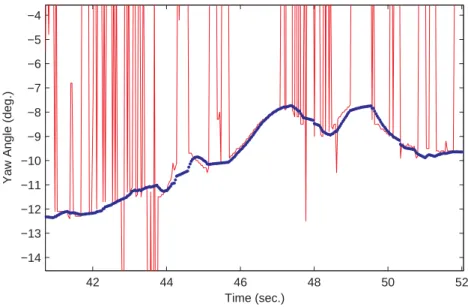
42 44 46 48 50 52 −14 −13 −12 −11 −10 −9 −8 −7 −6 −5 −4 Time (sec.)
Yaw Angle (deg.)
Figure 6: A comparison of predicted yaw and measured yaw.
6
Autopilot Performance
Some efforts were made to assess the effectiveness of the new autopilot. Due to the fact that the entire control algorithm was prototyped prior to implementa-tion, there were few surprises when the actual system was connected and used with the model in the offshore basin (OEB), with the controller performing as expected.
IOT had performed full-scale manoeuvring tests on the full-scale version of the model vessel recently, thus it was possible to derive the Nomoto steering parameters from this data. First-order wave filtering was not used during these tests. Since wave filtering requires that the wave estimator be tuned to the first order encounter frequency, there would have been considerable need for operator tuning because of the large number of possible combinations of vessel heading angles, wave directions and forward speeds. Instead, controller deadband was used to effect first order wave filtering.
6.1
Kalman Filter Performance
Figure 6 is a portion of a time-series plot from a model test. The Kalman filter’s predicted yaw (blue trace) fits the Qualisys signal (red trace), without including the errors and drop-outs.
Speed (kts.) Heading Angle (deg.) Yaw Angle (deg.) Min. Max. Std. Dev. 15 -7.063 9.941 2.288 35 -15.59 4.38 2.978 6.5 100 -5.65 4.96 1.51 125 -5.19 10.31 2.16 165 -9.11 6.809 2.309 15 -8.02 5.26 1.84 35 -9.69 4.63 2.03 9.5 105 -3.64 8.50 1.89 115 -4.48 4.48 1.47 155 -5.98 3.16 1.45 Table 1: Statistics for the actual heading angle versus set heading angle
6.2
Course-Keeping Performance
Generally, carrying out a seakeeping test within the confines of the OEB involves executing a number of runs which must be appended together to cover the specified wave spectrum - the number of segments is dependent on the direction with respect to the incident waves, the forward speed etc. This is one of the reasons that an autopilot is so important, since it ensures that each run is consistent with other runs of a particular heading.
A complex multi-directional sea state was generated, corresponding to data measured with a directional wave buoy during the full-scale seakeeping trials. The heading angles were derived after careful examination of the directional wave data as well as after reviewing the results of numerical simulations. The nominal target full scale wave parameters were 3.08 m significant wave height with a peak period of 11.8 s. A detailed description of these physical model experiments is described in the corresponding test report [3].
The autopilot provided satisfactory quality heading angle control regardless of model heading angle with respect to the incident waves - as indicated by reviewing the yaw angle statistics provided in table 1. The autopilot was able to maintain the set heading angle to within a maximum 2.98 degrees RMS. For the majority of runs, performance was much better- less than 2 degrees RMS. Although there was no direct comparison performed between this new system and previous model autopilots, it is felt that it provided control quality at least as good as previous systems. In addition, it would be difficult to compare this data to that of other models, since autopilot performance is also a function of the physical vessel, the test conditions and the controller tuning parameters (i.e. the controller gains).
7
Conclusions
The autopilot described in this report represents a great improvement over pre-vious autopilot systems. Its primary features are light weight and low power draw due to the absence of a large computer or gyroscope in the model. The incorporation of a Kalman filter allows a high-quality control solution to be computed in real-time from a noisy and unreliable feedback signal. The model for the Kalman filter is relatively simple to obtain and can be derived from either model scale or full scale steering data.
References
[1] R. G. Brown and P. Y. C. Hwang, Introduction to Random Signals and Applied Kalman Filtering. John Wiley and Sons, 1996.
[2] M. Grewal and A. Andrews, Kalman Filtering Theory and Practice. Prentice Hall, 1993.
[3] D. Cumming, D. Hopkins, and D. Bass, “Description of seakeeping and manoeuvring experiments carried out on M/V Louis M. Lauzier model IMD605,” Tech. Rep. TR-2003-15, Institute for Marine Dynamics, 2003. [4] T. Fossen, Guidance and Control of Ocean Vehicles. John Wiley and Sons,
1994.
[5] M. Morgan, Dynamic Positioning of Offshore Vessels. PPC Books, Division of Petroleum Publishing Company, 1978.
[6] G. Welch and G. Bishop, “An introduction to the kalman filter,” Tech. Rep. TR95-041, Department of Computer Science, University of North Carolina at Chapel Hill, 2003.
[7] D. Cumming, D. Hopkins, D. Williams, and G. Janes, “Description of ma-noeuvring, propulsion and seakeeping trials carried out on the M/V Louis M. Lauzier July - November 2001,” Tech. Rep. TR-2003-13, Institute for Marine Dynamics, June 2003.