Contents EmmanuelSchertzer FlorianSimatos HeightandcontourprocessesofCrump-Mode-Jagersforests(I):generaldistributionandscalinglimitsinthecaseofshortedges

(1)

E l e c t ro n ic J P r o b a b il i t y Electron. J. Probab. 23 (2018), no. 67, 1–43.

ISSN: 1083-6489 https://doi.org/10.1214/18-EJP151

Height and contour processes of Crump-Mode-Jagers forests (I):

general distribution and scaling limits in the case of short edges

Emmanuel Schertzer

*

_{Florian Simatos}

†

Abstract

Crump–Mode–Jagers (CMJ) trees generalize Galton–Watson trees by allowing individuals to live for an arbitrary duration and give birth at arbitrary times during their life-time. In this paper, we are interested in the height and contour processes encoding a general CMJ tree.

We show that the one-dimensional distribution of the height process can be expressed in terms of a random transformation of the ladder height process associated with the underlying Lukasiewicz path. As an application of this result, when edges of the tree are “short” we show that, asymptotically, (1) the height process is obtained by stretching by a constant factor the height process of the associated genealogical Galton–Watson tree, (2) the contour process is obtained from the height process by a constant time change and (3) the CMJ trees converge in the sense of finite-dimensional distributions.

Keywords: Crump-Mode-Jagers branching processes; Contour processes; Snakes; Bellman-Harris

pro-cesses; scaling limits.

AMS MSC 2010: 60J80; 60J85; 60J70; 60J75.

Submitted to EJP on July 22, 2016, final version accepted on February 14, 2018.

1 Introduction and statement of main results

1.1 Galton–Watson forests and their scaling limits.

A planar discrete rooted tree is a rooted tree where edges have unit length and which is endowed with an ordering on siblings, in such a way that it can be naturally embedded in the plane. Since the seminal work of Aldous, Neveu, Pitman and others [2, 3, 4, 17, 21, 22], it is well known that such a tree is conveniently encoded by its height and contour processes. To generate these processes, one can envision a particle starting from the root and traveling along the edges of the tree at unit speed, from left to right. The contour process is simply constructed by recording the distance of the particle from the root of the tree. To generate the height process, we start by labeling the vertices of the tree according to their order of visit by the exploration particle (i.e., from left to right): the height process evaluated at k is then given by the distance from the root of the kth vertex.

From a probabilistic standpoint, a particularly interesting case is the Galton–Watson case where each individual u in the tree begets a random number of offspringξu, these random variables

being i.i.d. with common distributionξ. In the critical and subcritical cases – i.e., when E(ξ) ≤ 1 – the tree is almost surely finite. Considering an infinite sequence of such i.i.d. random rooted planar trees, we can generate a random (planar) forest with its corresponding contour and height processes – respectively denoted byC and H – obtained by pasting sequentially the height and contour processes of the trees composing the forest.

WhenE(ξ2) < ∞, the large time behavior of those processes properly normalized in time and space can be described in terms of a reflected Brownian motion. More precisely, ifE(ξ) = 1 and if 0 < σ = Var(ξ2) < ∞ then we have

µ ₁

p_pH ([pt]),p1_pC (pt) ¶

=⇒ 2

σ (|w(t)|,|w(t/2)|)

with w a standard Brownian motion and the convergence holds weakly (in the functional sense), see Aldous [4], Bennies and Kersting [5] and Marckert and Mokkadem [19].

Le Gall and Le Jan [18] and then Duquesne and Le Gall [10] relaxed the finite variance assump-tion and proved, under suitable assumpassump-tions, the existence of a scaling sequence (_εp, p ∈ N) and a

limiting continuous pathH_∞such that ¡

εpH ([pt]),εpC (pt)¢ =⇒ (H∞(t ),H∞(t /2))

whereH_∞can be expressed as a functional of a spectrally positive Lévy process. In particular, we note that the height and contour processes are always asymptotically related by a simple deterministic and constant time change. The purpose of this paper is to extend these results to the more general class of Crump-Mode-Jagers forests.

1.2 Crump-Mode-Jagers forests

Chronological trees generalize discrete trees in the following way: each individual u is endowed with a pair (Vu,Pu) such that:

(3)

(2) Puis a point measure on (0, ∞) which represents the age of u at childbearing. As individuals

produce their offspring during their lifetime, we have_Pu(Vu, ∞) = 0.

Discrete trees are particular cases of chronological trees obtained with Vu= 1 and Pu= ξu²1, with

ξu∈ N the number of offspring and ²1the Dirac measure at 1.

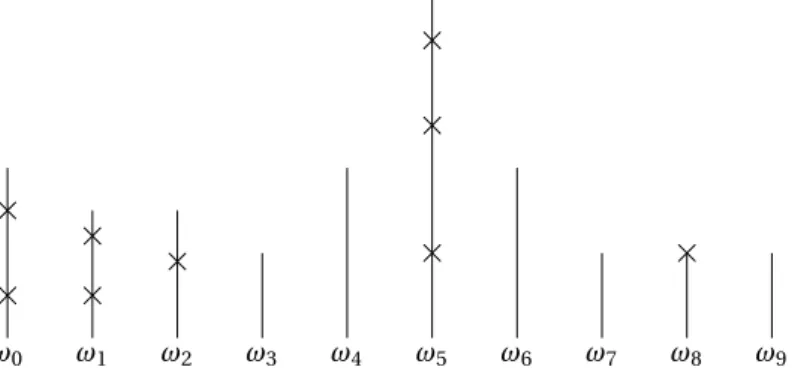
As noted by Lambert in [14] (to which the reader is referred for background on chronological trees), a chronological tree can be regarded as a tree satisfying the rule “edges always grow to the right”. This is illustrated in Figures 1 and 2 where we present a sequential construction of a planar chronological forest from a sequence of “sticks”ω = (ωn, n ≥ 0), where ωn= (Vn,Pn).

ω0 ω1 ω2 ω3 ω4 ω5 ω6 ω7 ω8 ω9

Figure 1: Sequence of sticks used in the next figures: this sequence corresponds to one chronologi-cal tree.

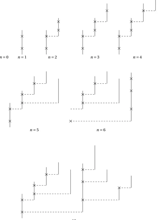
1.2.1 Sequential construction of a Crump-Mode-Jagers forest

The reader is refered to Figures 1 and 2 for an illustration of this construction.

At time n = 0 we start with the empty forest and we add the stick ω0at time n = 1. In the case

considered in Figure 2,P0has two atoms which correspond to birth times of individuals, but

these two atoms are not yet matched with the sticks corresponding to these individuals. These unmatched atoms are called stubs, and each time there is at least one stub we graft the next stick to the highest stub.

We iteratively apply this rule until there is no more stub, at which point we have built a complete chronological tree with a natural planar embedding. Figure 2 illustrates a particular case where at time 10 there is no more stub, and in each time this happens we start a new tree with the next stick.

Thus, starting at time n = 0 from the empty forest and iterating these two rules, we build in this way a forest_F∞_{, possibly consisting of infinitely many chronological trees. By definition, a}

CMJ forest is obtained when the initial sticks are i.i.d., and throughout the paper we will denote their common distribution by (V∗,P∗).

1.2.2 Chronological height and contour processes of CMJ forests

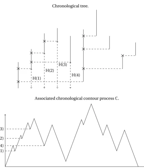
As for discrete trees, the contour process of a CMJ forest is obtained by recording the position of an exploration particle traveling at unit speed along the edges of the forest from left to right, moving, when a chronological tree is represented as in Figure 2, at infinite speed along dashed lines. This process will be referred to as the chronological contour process associated to the CMJ forest, and the chronological height of an individual is defined as its date of birth.

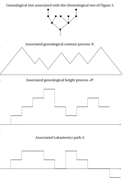
We define the genealogical contour and height processes as the contour and height processes associated to the discrete forest encoding the genealogy ofF∞, see Figures 3 and 4 for a pictorial representation. Throughout the paper, we use the following notation:

Genealogical processes :H and C denote the genealogical height and contour processes,

(4)

n = 0 n = 1 n = 2 n = 3 n = 4

n = 5 n = 6

n = 10

Figure 2: Sequential construction of the chronological tree from the sequence of sticks of Figure 1: as long as there is a stub availabe, we graft the next stick at the highest one. At n = 10 the construction is complete (there is no more stub available) and the next stick will therefore start the next tree in the forest.

Chronological processes :H and C denote the chronological height and contour processes,

(5)

Chronological tree.

H(1) H(2)

H(3) H(4)

Associated chronological contour processC.

H(1) H(2) H(3)

H(4)

Associated chronological height processH.

H(1) H(2) H(3)

H(4)

Figure 3: Chronological height and contour processes associated to the chronological tree con-structed from the sequence of sticks of Figure 1.

Contour processes of CMJ forests have been considered by Lambert in [14] in the particular setting where birth events are distributed in a Poissonian way along the sticks independently of the

(6)

Genealogical tree associated with the chronological tree of Figure 3.

Associated genealogical contour processC .

Associated genealogical height processH .

Associated Lukasiewicz path S.

Figure 4: The genalogical tree of the chronological tree of Figure 3, together with the genealogical processes S,_{H and C . The genealogical tree is obtained by applying the mapping G to the initial} sequence of sticks, which amounts to resizing all the sticks to unit size and putting all the atoms at one. The (genealogical) height and contour processes are then obtained as before, but from the genealogical tree. Note on the genealogical tree the additional edge compared to the usual associated discrete tree displayed in Figure 7.

life-length – the so-called binary, homogeneous case. Under this assumption, the author showed that the (jumping) contour process is a spectrally positive Lévy process. See also [8, 9, 15, 16, 23, 24] for related works.

1.3 Overview of main results

Besides these results, little is known to our knowledge in the general case. One of the main result of the present paper is to describe in full generality the joint distribution of the chronological

(7)

and genealogical height processes at a fixed time, see Theorem 1.1 and Lemma 2.12 below. We believe that this description paves the way to a general study of Crump-Mode-Jagers forests. As an illustration, we treat here the so-called “short edge” case where edges of the chronological trees are short: in this case, the Crump-Mode-Jagers forest becomes asymptotically proportional to its genealogical forest. This loose statement is formalized in Theorems 1.5, 1.10 and and 1.12 below.

Also, in current work in progress [31] we use these techniques to treat the case where the offspring distribution has finite variance: in this case, new scaling limits emerge, which are related to the Poisson snake [1, 6].

1.4 First main result: joint distribution of the chronological and genealogical height pro-cesses at a fixed time.

Recall that all our objects are constructed from an initial sequence of sticks (ωn, n ≥ 0) with ωn= (Vn,Pn). Let S = (S(n),n ∈ N) be the Lukasiewicz path of (|Pn|): it is defined by S(0) = 0 and,

for n ≥ 1, S(n) = n−1 X k=0 (|Pk| − 1)

(here and in the sequel, |ν| is the mass of the measure ν). Let T = (T (k),k ∈ N) be the sequence of weak ascending ladder height times, also referred to as record times: it is defined by T (0) = 0 and by

T (k + 1) = inf©

` > T (k) : S(`) ≥ S(T (k))ª

for k ≥ 0, with the convention T (k + 1) = ∞ if T (k) = ∞. Let eT−1_{(n) for n ∈ N be the number of}

record times smaller than n, i.e.,Te−1(n) = max{k ≥ 0 : T (k) ≤ n}. For k ≥ 1 such that T (k) < ∞, define

ξ(k) = S(T (k − 1)) − S(T (k) − 1)

corresponding to the undershoot upon reaching the kth record time. For any measureP and any

k ≤ |P |, denote by Ak(P ) the position of the kth largest atom of P .

As explained above, all our objects are constructed from an initial sequence of sticksω = (ωn, n ∈ N). For technical convenience, we actually assume that a sequence of sticks ω is indexed

byZ, i.e.,ω = (ωn, n ∈ Z), and we denote by Ω the set of sequences of sticks. This makes it

possible to consider, for each n, the dual (or time-reversal) operatorϑn :Ω → Ω defined by

ϑn₍_{ω) = (ω}

n−k−1, k ∈ Z). Recall that H is the height process of a classical Galton-Watson tree.

Our first main result is the following one: its proof is presented in Section 2.5. In the following statement, Ak(ν) is the position of the kth largest atom of the point measure ν.

Theorem 1.1.For n ∈ N let

R(n) = X

1≤k≤n:T (k)<∞

Y(k) where Y(k) = Aξ(k)(PT (k)−1).

Then the genealogical and chronological height processes at time n are given by the following formula:

¡

H (n), H(n)¢ = ¡Te−1(n) , R ◦ eT−1(n)¢ ◦ ϑ

n_. _(1.1)

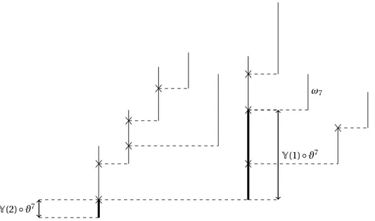
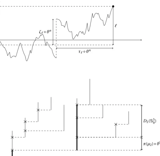
The functionalY(k) ◦ ϑn appearing in the above statement is depicted in Figures 5 and 6. Moreover, the functionals in the right-hand side of (1.1) are by definition computed with respect to the reversed sequence of sticks (ω_n−k−1, k ∈ Z), e.g., eT−1(n) ◦ ϑnis the nth record time associated to the sequence (ωn−1−k, k ≥ 0).

We note that the one-dimensional marginals of the genealogical height processH in terms of the ladder height time process is already known in the literature, see for instance Marckert and Mokkadem [19]. The previous result states that in order to describe the chronological height process, more structure of the ladder height process is needed: not only do we need to extract the

(8)

ω7

Y(2) ◦ ϑ7

Y(1) ◦ ϑ7

Chronological tree with the spine of the 7th individual in thick lines.

S7

0= ( , )

Value of the spine process at time n = 7.

Figure 5: Illustration of the random variablesY(k) ◦ ϑnand of the spine processSn₀: the figure presents these objects for n = 7. The 7th individual has two ancestors, so the spine process at time

n is of length 2 and is made, according to Proposition 2.4, of the two measures corresponding to

the thick lines in this figure. The random variableY(1) ◦ ϑn_{= S}n₀(2) records the part of the life of the first ancestor that is currently or has not been visited yet,Y(2) ◦ ϑn_{= S}n₀(1) the part of the life of the second ancestor that is currently or has not been visited yet.

record times (as in the Galton-Watson case), but also the corresponding undershoots.

We emphasize the fact that the previous result is purely deterministic. We now introduce the probabilistic set-up of Crump-Mode-Jagers forests and state our main results concerning the asymptotic behavior of the chronological height and contour processes.

1.5 Main results: scaling limits

We now present the main results of the paper concerning the asymptotic behavior of the chronological height and contour processes, see Theorems 1.5, 1.10 and 1.12 below.

1.5.1 Probabilistic set-up

A Crump-Mode-Jagers forest is obtained when the initial sequence of sticks is i.i.d.. We consider in this paper a triangular setting and consider for each p ≥ 1 a stick-valued random variable (Vp∗,Pp∗)

(9)

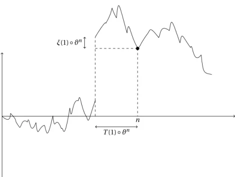
n T (1) ◦ ϑn ξ(1) ◦ ϑn

Figure 6: The n − T (k) ◦ ϑnare n’s ancestors. To compute the contribution of the kth ancestor to the spine of n, i.e., to computeSn₀(H (n) − k) = Y(k) ◦ ϑn, we do as follows:

• look at the Lukasiewicz path backward in time from n and stop at the kth record time

T (k) ◦ ϑn;

• in the construction of the chronological tree, this time corresponds to the addition of the stickP_{T (k)−1}◦ ϑn;

• the overshoot (for the process forward in time)ξ(k) ◦ ϑnrepresents the number of children of the kth ancestor of n that have already been explored;

• thus, the remaining contribution of this ancestor to the spine is obtained by deleting this number of atoms fromP_{T (k)−1}◦ ϑn.

corresponding to a (sub)critical CMJ branching process, i.e., which satisfies

0 ≤ E(|Pp∗|) ≤ 1. (1.2)

We assume moreover that the sequence (P_p∗) is near-critical in the sense that lim

p→∞E(|P

∗

p|) = 1. (1.3)

LetPp be the probability distribution onΩ under which ω is an i.i.d. sequence of sticks with

common distribution (V_p∗,P_p∗). We let ⇒ denote weak convergence under Pp and

fdd

⇒ denote convergence in the sense of finite-dimensional distributions underPp. That is, Bp

fdd

⇒ B∞if and

(10)

1.5.2 Preliminaries

For a given sequence (εp, p ∈ N), define the rescaled processes Hp,Hp, Sp,CpandCpas follows:

for t ∈ R+:

Hp(t ) = εpH ([pt]), Hp(t ) = εpH([pt]) and Sp(t ) =

1

p_εp

S([p t ]), (1.4)

([x] ∈ Z denotes the integer part of x ∈ R) and

Cp(t ) = εpC (pt), Cp(t ) = εpC(pt). (1.5)

In the near-critical case, it is well-known since Duquesne and Le Gall [10] that if Spconverges, then

under under additional mild assumptions the rescaled genealogical height and contour processes converge weakly toward a continuous process. This is summarized in the next theorem which involves the following condition.

Condition 1.2.G The following three conditions are met: (H1) Sp⇒ S∞for some Lévy process S∞with infinite variation;

(H2) the Laplace exponentψ of S_∞satisfiesR∞

1 du/ψ(u) < ∞;

(H3) if (Z_kp, k ≥ 0) is a Galton-Watson process with offspring distribution |P∗

p| and started with

[pεp] individuals, then for everyδ > 0,

lim inf p→∞ P ³ Zp [δ/εp]= 0 ´ > 0.

Note that Grey’s condition (H2) implies that the corresponding continuous state branching process gets almost surely extinct [13]. When condition 1.2 holds, we can and will assume without loss of generality that as p → ∞ we have εp→ 0 and pεp→ ∞. Moreover, since we are in triangular

setting where the law of the jump size of S may depend on p, S_∞is not necessarily a stable process.

Theorem 1.3 (Corollary2.5.1 in [10]). Assume that condition 1.2 holds. Then (Hp,Cp) ⇒

(H_∞,H_∞( ·/2)) for some continuous process H∞satisfyingP(H∞(t ) > 0) = 1 for every t > 0. 1.5.3 Convergence of the chronological height process

To explain our results we start with some notation. The strong Markov property implies that the random variablesY(k) introduced in Theorem 1.1 are i.i.d. (under Pp), and we denote byY∗pa

random variable with their common distribution. We will show in Lemma 2.12 thatY∗

pis obtained

by first size-biasing the random variable |Pp∗| and then recording the age of the individual when

giving birth to a randomly chosen child. The mean ofY∗_phas a simple expression, namely (see Lemma 2.12) E(Y∗ p) = E µZ ∞ 0 uP_p∗(du) ¶ . (1.6)

Nerman and Jagers [20] already noticed thatY∗

pdescribes the age of an ancestor of a typical

indi-vidual when giving birth to its next ancestor. For this reason,Y∗

pand in particular the condition

E(Y∗

p) < ∞ – which is one way to formalize the “short edge” condition – plays a major role in

previ-ous works on CMJ processes, see for instance [25, 26, 27, 28, 29, 30]. In the present paper we prove that ifE(Y∗_p) < ∞, then in the near-critical regime the asymptotic behavior of the chronological height process is obtained by stretching the genealogical height process by the deterministic factor E(Y∗

p). The statement involves the following assumption which is alway satisfied (under (1.3)) in

the non-triangular setting. The proof of this result is the content of Section 3.

Condition 1.4.Y The sequence of random variables (Y∗_p) is uniformly integrable and converges

(11)

Theorem 1.5 (Short edges).Assume that conditions 1.2 and 1.4 hold. Then ¡ Hp,Hp¢ fdd =⇒¡ H∞,α∗H∞¢ .

Remark 1.6.Theorem 1.5 is a consequence of a more general result: if, for a fixed t ,Hp(t ) is

tight and a weaker condition than condition 1.4 holds, thenHp(t ) − Hp(t ) ⇒ 0, see Theorem 3.1

below.

Remark 1.7.In [29], Sagitov investigated (in the non-triangular setting) the size of a CMJ process conditioned to survive at large time under the very short edge assumption introduced below, corresponding toE(V₁∗) < ∞ and E(Y∗1) < ∞ (see also Section 8 and Green [12]). The population

size is described in the limit in terms of a continuous state branching process where space and time are scaled analogously as in Theorem 1.3. As a consequence, the previous result can be seen as a genealogical version of [29]. We also note that in [29], the results are obtained through an entirely different approach, namely analytic computations involving some non-trivial extension of the renewal theorem.

1.5.4 Convergence of the chronological contour process

The analysis of the contour process is significantly more delicate than that of the height process: compared to the Galton–Watson case, new difficulties are created by the chronological structure, see the discussion in Section 1.6.

For the chronological contour process, condition 1.4 is not enough. Indeed, we note thatH does not “see” what happens after an individual has given birth to its last child. In other words, two sequences of sticksω = ((Vn,Pn), n ∈ Z) and ˜ω = (( ˜Vn, ˜Pn), n ∈ Z) yield the same chronological

height process as soon asPn= ˜Pn. In contrast, the chronological contour process heavily depends

on the life length of individuals and so an extra assumption on V∗

p is called upon.

Condition 1.8.VP The sequence of random sticks (V_p∗,P_p∗) converges in law to a random stick (V∗

∞,P∞∗) such that V∞∗has meanE(V∞∗) = β∗∈ (0, ∞) and E(|P∞∗|) = 1. Moreover, the sequence (Vp∗) is uniformly integrable.

We will repeatedly use the following direct consequence of the convergence V_p∗⇒ V∞∗with the

(V∗

p) uniformly integrable, see for instance [11, §22].

Lemma 1.9.For any sequence up→ ∞ we have V ([up])/up⇒ β∗. In particular, for any t ≥ 0 we have_{V ([pt])/p ⇒ β}∗_{t .}

In light of the above discussion, condition 1.8 is intuitively more stringent than condition 1.4 and so we will refer to this case as to the case of “very short edges”1. Our main result shows that when conditions 1.4 and 1.8 hold, then the chronological contour process is obtained from the chronological height process by rescaling time by the deterministic factor 1/(2β∗_{). Hence,}

again provided that edges are short enough, this result provides a relation between the height and contour processes which is analogous to the discrete case. Moreover, the limits are proportional to the height process (up to multiplicative constant in time and space) of a continuous-state branching process as in the Galton-Watson case. The following result is proved in Section 4.

Theorem 1.10 (Very short edges case).Assume that conditions 1.2, 1.4 and 1.8 hold. Then

¡ Hp,Cp,Hp,Cp ¢ fdd =⇒¡H∞,H∞( ·/2),α∗H∞,α∗H∞◦ ϕ∞ ¢ whereϕ_∞(t ) = t/(2β∗).

Remark 1.11.Theorem 1.10 is a consequence of a more general result: if only condition 1.8 holds (with no requirement onY∗_p), then the contour process can be obtained from the height process by a deterministic time change, see Theorem 4.1 below.

1_{It follows from (1.6) that}_E(Y∗_{) ≤ E(V}∗_|P∗_{|) and so if the life length is independent from the number of offspring, then}

(12)

The previous result, and in particular the joint convergence (Cp,Cp)

fdd

⇒ (H∞( ·/2),α∗H∞◦ ϕ∞),

strongly suggests that the whole chronological forest can asymptotically be obtained from the genealogical one through a deterministic stretching of the edges. If instead of convergence of finite-dimensional marginals we had functional convergence in the previous display, then this would actually be exact. However, we exhibit counter-examples in Section 8 where the assump-tions of Theorem 1.10 hold, but there cannot be functional convergence. Despite this negative result, the following result shows that the chronological and genealogical forests indeed become asymptotically proportional to one another in the sense of finite-dimensional distributions. The following result is proved in Section 7.

Theorem 1.12.Assume that conditions 1.2, 1.4 and 1.8 hold. Then for every 0 ≤ u ≤ v we have

inf

u≤t≤vCp(t ) − α

∗ _inf

u≤t≤vCp(2ϕ∞(t )) ⇒ 0.

1.6 Main ideas of the proof of Theorems 1.5 and 1.10 and technical challenges

The proof of Theorem 1.5 is actually quite straightforward once Theorem 1.1 is established. Indeed, condition 1.4 implies that the law of large numbers hold for R. It gives R(n) ≈ α∗n for

large n and as a consequence,

H(n) = R ◦Te−1(n) ◦ ϑ

n

≈ α∗Te−1(n) ◦ ϑ

n

= α∗H (n)

(note that since we are interested in convergence in distribution, the dual operator is actually irrelevant). Details are provided in Section 3.

In contrast, the proof of Theorem 1.10 is significantly more difficult. To explain this difficulty, it is useful to compare with the Galton–Watson case.

1.6.1 The Galton-Watson case

In the Galton-Watson case, the convergence of the contour process is obtained from the conver-gence of the height process by using the fact that the contour process somehow interpolates the height process (see details below). This observation leads to the inequality (see for instance [10, Equation (2.33)]) sup 0≤s≤t ¯ ¯C_p(s) − H_p( f_p(s)) ¯ ¯≤ ε_p+ sup s≤t ¯ ¯H_p(s + 1/p) − H_p(s) ¯ ¯ (1.7) with fp(t ) = 1 pinf© j ≥ 0 : 2(j − 1) − H (j ) ≥ ptª.

Because_{H (j) ¿ j, it is not hard to see that f}p converges (in a functional sense) to the linear

function t 7→ t/2. From (1.7), it is obvious that if Hp⇒ H∞, again in a functional sense, withH∞

continuous, thenHpandCpconverge jointly.

1.6.2 The Crump-Mode-Jagers case

Many of these ideas work in the present chronological setting, and we begin by explaining the interpolation alluded above. We define in the sequel

V (−1) = 0, V (n) = V0+ · · · + Vn and Kn= 2V (n − 1) − H(n), n ≥ 0.

Note that the sequence (Kn, n ≥ 0) is non-decreasing and that its terminal value is almost surely

infinite (because of the subcritical assumption (1.2)). It can be checked from the definition of the chronological height and contour processes that:

(13)

• C(Kn) = H(n) for every n ∈ N;

• for t ∈ [Kn, Kn+1],C first increases at rate +1 up to H(n) +Vnand then decreases at rate −1

toH(n + 1).

SinceH(n +1) ≤ H(n)+Vnand Vn+ (Vn+ H(n) − H(n + 1)) = Kn+1− Kn, this interpolation is indeed

well-defined. Moreover, it immediately entails the following bound (see for instance Figure 3, and note that it holds deterministically for any initial sequence of sticks):

sup

t ∈[Kn,Kn+1]

|C(t) − H(n)| ≤ |H(n + 1) − H(n)| +Vn. (1.8)

Let furtherϕ be the left-continuous inverse of (K[t ], t ≥ 0), defined by

ϕ(t) := min©j ≥ 0 : Kj≥ tª , t ≥ 0. (1.9) Then defining ϕp(t ) := 1 pϕ(pt) = 1 pinf© j ≥ 0 : 2V (j − 1) − H(j ) ≥ ptª, (1.10)

the inequality (1.8) translates after scaling into ¯ ¯Cp(t ) − Hp(ϕp(t )) ¯ ¯≤ εpVϕ(pt)+¯¯Hp(ϕp(t ) + 1/p) − Hp(ϕp(t )) ¯ ¯, t ≥ 0, (1.11) which is the chronological generalization of (1.7). Under condition 1.8, the law of large numbers applies toV and gives V (j − 1) ≈ β∗j . AsH(j) ¿ j, this gives similarly as in the Galton-Watson

caseϕp(t ) ⇒ ϕ∞(t ). However, the analogy with the Galton-Watson case stops here, and we now

highlight the main differences with the Galton-Watson case, and the technical challenges to overcome in order to prove Theorem 1.10.

1.6.3 Difference with the Galton-Watson case

First of all, although in the Galton-Watson case the gap between convergence of finite-dimensional distributions and functional convergence ofHpis small (this is essentially condition (H2) above,

and this can only happen in a triangular setting) this is not the case for the chronological height process. To illustrate this, we present in Section 8 simple non-triangular examples whereHp

converges in the sense of finite-dimensional distributions but the limiting process is unbounded on any open interval. For this to happen in the Galton-Watson case, one has to consider very specific offspring distributions in a triangular setting (so that condition (H2) above does not hold), whereas here many simple examples, in a non-triangular setting, can be easily found. In other words, assuming functional convergence ofHpseems a strong hypothesis to make; and finding conditions under which_Hpconverges in a functional sense constitutes an interesting open

problem which is not addressed here. More deranging, we also exhibit in Section 8 an example whereHpconverges in a functional sense to a continuous process, butCpfails to converge in a

functional sense.

These various examples show that the usual techniques developed in the Galton-Watson case are insufficient, and new arguments are called upon.

1.6.4 Technical challenges and new arguments

Technically, one of the main difficulty comes from the fact that the random timeϕp(t ) appearing

in (1.11) is not “nice”: because the processesV and H appearing in its definition are dependent, we cannot readily rely on renewal-type arguments to control it, or to control other processes considered at this time. For instance, even the termεpVϕ(pt)appearing in the right-hand side

(14)

in the Galton-Watson case), is actually not straightforward to control and involved arguments are needed (see Section 6.3).

To circumvent this problem, the main idea is to approximateϕ by a “nicer” random time ¯ϕ: since, as mentioned above,V (j) À H(j), a natural approximation of ϕ is given by

¯

ϕ(t) = inf©j ≥ 0 : 2V (j) ≥ tª.

It turns out that ¯ϕ indeed exhibits many useful properties and that the other processes are much easier to control when considered at ¯ϕ than at ϕ. For instance, 2Vϕ(pt)¯ is the jump of the

re-newal process 2V straddling pt, and can thus be controlled by the renewal theorem. As another illustration, we will show in Lemma 6.6 thatH shifted at ¯ϕ has a simple and useful probabilistic description (which is not the case forH shifted atϕ).

Thus, the global idea of the proof is to: • show that ¯ϕ and ϕ are close;

• use this to transfer problems onϕ to problems on ¯ϕ; • leverage the nicer structure of ¯ϕ to solve problems on ¯ϕ.

In addition, one of the main ingredient to fulfill this program is a refined decomposition of the spine of an individual. This decomposition relies on the spine process, which generalizes the exploration process of Le Gall and Le Jan in [18] to the present chronological setting. This process lies at the heart of the proof of Theorem 1.1 and of many other results: it is presented in the next section.

1.7 Notation

Before going on we collect some general notation used throughout the paper.

1.7.1 General notation

LetZ denote the set of integers and N the set of non-negative integers. For x ∈ R let [x] = max{n ∈ Z : n ≤ x} and x+_{= max(x, 0) be its integer and positive parts, respectively. If A ⊂ R is a finite}

set we denote by |A| its cardinality. Throughout we adopt the convention max; = sup; = −∞, min ; = inf; = +∞ andPb

k=auk= 0 if b < a, with (uk) any real-valued sequence.

1.7.2 Measures

LetM be the set of finite point measures on (0,∞) endowed with the weak topology, ²x∈ M

for x > 0 be the Dirac measure at x and z be the zero measure, the only measure with mass 0. For a measureν ∈ M we denote its mass by |ν| = ν(0,∞) and the supremum of its support by

π(ν) = inf{x > 0 : π(x,∞) = 0} with the convention π(z) = 0. For k ∈ N we define Υk(ν) ∈ M as the

measure obtained by removing the k largest atoms ofν, i.e., Υk(ν) = z for k ≥ |ν| and, writing ν = P|ν|

i =1²a(i )with 0 < a(|ν|) ≤ ··· ≤ a(1), Υk(ν) = P|ν|_{i =k+1}²a(i )for k = 0,...,|ν| − 1.

1.7.3 Finite sequences of measures

We letM∗= ∪n∈N(M \ {z})n be the set of finite sequences of non-zero measures inM . For Y ∈ M∗_{we denote by Len (Y ) the only integer n ∈ N such that Y ∈ (M \ {z})}n_{, which we call}

the length of Y , and identify z with the only sequence of length 0. For two sequences Y1=

(Y1(1), . . . , Y1(H1)) and Y2= (Y2(1), . . . , Y2(H2)) inM∗with lengths H1, H2≥ 1, we define [Y1, Y2] ∈

M∗_{as their concatenation:}

(15)

Further, by convention we set [z, Y ] = [Y ,z] = Y for any Y ∈ M∗and we then define inductively [Y1, . . . , YN] =£[Y1, . . . , YN −1], YN¤, N ≥ 2.

Note that, with these definitions, we have Len ([Y1, . . . , YN]) = Len(Y1) +···+Len(YN) for any N ≥ 1

and Y1, . . . , YN∈ M∗.

Identifying a measureν ∈ M \ {z} with the sequence of length one (ν) ∈ M∗_{, the above}

def-initions give sense to, say, [Y ,ν] with Y ∈ M∗andν ∈ M \ {z}. The operator π defined on M is extended toM∗through the relation

π(Y ) =Len(Y )X

k=1

π(Y (k)), Y = (Y (1),...,Y (Len(Y )) ∈ M∗_.

Recalling the conventionP0

k=1= 0, we see that π(z) = 0 and further, it follows directly from the

above relation thatπ([Y1, . . . , YN]) = π(Y1) + ··· + π(YN).

1.7.4 Measurable space

We defineL = {(v,ν) ∈ (0,∞) × M : v ≥ π(ν)} and call an element s ∈ L either a stick or a life

descriptor. We work on the measurable space (Ω,F ) with Ω = LZthe space of doubly infinite sequences of sticks andF the σ-algebra generated by the coordinate mappings. An elementary eventω ∈ Ω is written as ω = (ωn, n ∈ Z) and ωn = (Vn,Pn). For n ∈ Z we consider the three

operatorsθn,ϑn,G : Ω → Ω defined as follows:

• θnis the shift operator, defined byθn(ω) = (ωn+k, ∈ Z);

• ϑnis the dual (or time-reversal) operator, defined byϑn(ω) = (ω_n−k−1, k ∈ Z);

• G is the genealogical operator, mapping the sequence ((Vn,Pn), n ∈ Z) to the sequence

((1, |Pn|²1), n ∈ Z).

Note that the genealogical and chronological height and contour processes are related by the relationsH = H ◦ G and C = C ◦ G . We say that a mapping Γ : Ω →X(valued in an arbitrary space

X) is a genealogical mapping if it is invariant by the genealogical operator, i.e., ifΓ ◦ G = Γ. The shift and dual operators are related by the following relations:

ϑm

◦ ϑn= θn−m and ϑn◦ θm= ϑn+m, m, n ∈ Z, (1.12)

and for any random timeΓ : Ω → Z we have

PΓ◦ ϑn= Pn−1−Γ◦ϑn. (1.13)

Remark 1.13.To be completely rigorous, our genealogical contour process differs from the one usually considered in the literature. The difference comes from the fact that when applying the genealogical operator, the corresponding tree starts with an edge corresponding to the life of the root as in Figure 4. In contrast, the discrete trees usually considered do not have this edge, cf. Figure 7. It is straightforward to check that the genealogical results which we use here (in particular, those in Duquesne and Le Gall [10]) continue to hold with this modified contour process.

2 Spine process and Lukasiewicz path

In this section, we introduce the spine process and relate it to the well-known Lukasiewicz path. The spine process is introduced in Sections 2.1 and 2.2 and the Lukasiewicz in Section 2.4. We prove in Section 2.5 a crucial formula for the spine process (see Proposition 2.4) from which Theorem 1.1 is readily derived. More precisely, the spine process is expressed in terms of a random functional of the weak ascending ladder height process associated to the dual Lukasiewicz path. Sections 2.6 and 2.7 continue the study of the spine process and give a description of the.

(16)

Figure 7: Usual discrete tree associated with the chronological tree of Figure 3.

2.1 Overview of the spine process

The idea underlying the definition of the spine process relies on the decomposition of the “spine” – or “ancestral line” – lying below the point of the tree corresponding to the birth of the nth individual. In the nth step of the sequential construction presented on Figure 2, this corresponds to the path in the forest starting from the root and reaching up to n (which also corresponds to the right-most path in the planar forest constructed at step n). As can be seen from the figure, this path is naturally decomposed into finitely many segments that correspond to each ancestor’s contribution to the spine: these segments are highlighted in bold on Figure 8. See also Figure 9.

The spine process at n is then defined as a sequence of measures that encodes this decomposi-tion. More precisely, we start by labeling ancestors from highest to lowest. Then, the kth element of the spine process (evaluated at time n) is simply the measure that records the location of the stubs on the kth segment – crosses on Figure 8 – and the age of the kth ancestor upon giving birth to the (k − 1)st ancestor – circles on Figure 8.

2.2 Spine process

Consider the operatorΦ : M∗_{× M → M}∗defined forν ∈ M and Y = (Y (1),...,Y (Len(Y )) ∈ M∗_by Φ(Y ,ν) =        [Y ,ν] ifν 6= z, ¡Y (1),...,Y (H − 1),Υ1(Y (H )) ¢ ifν = z and H ≥ 1, z else, (2.1)

where H = max{k ≥ 1 : |Y (k)| ≥ 2}. Note that by definition, we have Φ(Y ,ν) ∈ M∗for Y ∈ M∗and

ν ∈ M and that further, if ν 6= z then Φ(Y ,ν) 6= z.

The spine processS0= (Sn₀, n ≥ 0) (the subscript 0 will be justified below, see (2.9)) is the

M∗_{-valued sequence defined recursively by}

S0

0= z and Sn+10 = Φ(S

n

0,Pn), n ≥ 0. (2.2)

This dynamic is illustrated on Figure 8. As already discussed in the introduction, the kth element ofSn₀(ordered from top to bottom) records (1) the location of the stubs on the kth segment in the spine decomposition illustrated in Figure 8, and (2) the age of the kth ancestor (of n) when begetting the (k − 1)st ancestor (identifying, for k = 1, the individual with its 0th ancestor). In words, the recursive relation (2.2) encodes the fact that the birth event corresponding to the (n + 1)st individual coincides with the next available stub after grafting the nth stick on top of Sn0.

In particular, if no stub is available, a new spine is started from scratch (third relation).

We note that whenSn₀6= z, any element of the sequence Sn0contains at least one atom: the one

corresponding the birth of an ancestor, which is not counted as a stub. In particular, the condition

H = max{k ≥ 1 : |Y (k)| ≥ 2} in (2.1) reads “look for the first available segment with a stub”.

2.3 Link between the spine process and the height and exploration processes

As discussed above, the spine process encodes the spine of an individual by breaking it into the different sticks of its ancestors as in Figure 8. In particular, the birth time of the individual is recovered by summing up the lengths of the sticks appearing in the spine process: this means

(17)

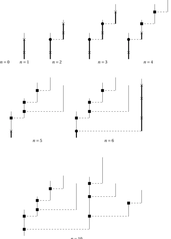
n = 0 n = 1 n = 2 n = 3 n = 4

n = 5 n = 6

n = 10

Figure 8: Same construction as in Figure 2, but now with the spine highlighted in thick line. This allows to differentiate three kinds of atoms:

Cross represents a stub and corresponds to an atom on the spine whose subtree has not been

explored yet;

Circle represents an atom on the spine whose subtree is being explored;

(18)

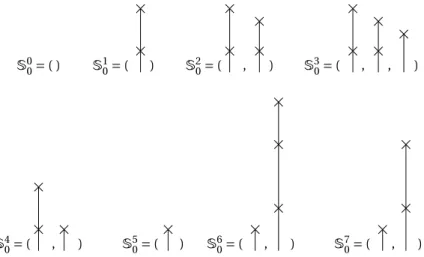
S0 0= ( ) S 1 0= ( ) S 2 0= ( , ) S 3 0= ( , , ) S4 0= ( , ) S50= ( ) S60= ( , ) S70= ( , )

Figure 9: Evolution of the spine process for n = 0,...,6. At each time, the sequence of sticks (for instance, making upS4₀) is made up of the thick lines, together with their atoms, of Figure 8, and soSn₀indeed encodes the spine of n.

This sequence can also be obtained by iteration of the dynamic (2.1) to the initial sequence of sticks of Figure 1: each time, either we add a new stick, or if the next stick has no atom, we remove the highest stub of the current last stick (possibly iteratively, thereby removing several sticks at once).

In the classical exploration process of Le Gall and Le Jan, one only counts the number of stubs (minus one, since we know that there must be at least one): one does not need to record their positions since they are all at the deterministic location one.

precisely that the spine process and the chronological height process are related as follows: H(n) = π(Sn

0), n ≥ 0.

The spine process can be seen as a chronological generalization of the exploration process of Le Gall and Le Jan [18], and for this reason we will define_ρn₀_{= S}n₀_{◦ G as the exploration process.} This process is not exactly the one of Le Gall and Le Jan. Therein, the authors only consider the stubs attached to the spine. However, in the chronological case, not only do we need to keep track of the number of available stubs, but one needs to also record the length of the segments carrying those stubs (in the discrete case, this is always equal to 1). This is done by adding the additional atom corresponding to the birth of the “previous” ancestor (when ancestors are labelled from top to bottom), and whose location coincides with the length of the corresponding segment.

2.4 Lukasiewicz path

Recall that we already introduced some notation in the introduction. We define the Lukasiewicz path S = (S(n),n ∈ Z) by S(0) = 0 and, for n ≥ 1,

S(n) = n−1 X k=0 (|Pk| − 1) and S(−n) = − −1 X k=−n (|Pk| − 1) .

Note that ifΓ is a random time, the dual operator acts as follows (recall that ϑ is defined in Section 1.7):

S(_{Γ) ◦ ϑ}n_{= S(n) − S(n − Γ ◦ ϑ}n_{), n ∈ Z.} (2.3) We consider the following functionals associated to S, which will be used repeatedly in the rest of the paper:

(19)

• the sequence of weak ascending ladder height times: T (0) = 0 and for k ≥ 0,

T (k + 1) = inf©

` > T (k) : S(`) ≥ S(T (k))ª = T (1) ◦ θT (k)+ T (k);

• the hitting times upward and downward:

τ`= inf{k > 0 : S(k) ≥ `} and τ−`= inf{k ≥ 0 : S(k) = −`} , ` ≥ 0,

so that in particularτ0= T (1);

• for` ∈ N with τ_`_{< ∞,}

ζ`= ` − S(τ`− 1) and µ`= Υζ`(Pτ`−1),

so thatζ_`is the undershoot upon reaching level`; • and the backward maximum

L(m) = max

k=0,...,mS(−k), m ≥ 0.

Note that, since S(τ0) ≥ 0, ζ0= −S(τ0− 1) ≤ S(τ0) − S(τ0− 1) = |Pτ0−1| − 1, so that µ06= z. We will pay special attention to the following functionals of the ladder height process:

• for k ≥ 1 with T (k) < ∞ (recall that Ak(ν) is the position of the kth largest atom of ν),

Q(k) = µ0◦ θT (k−1) and Y(k) = π ◦ Q(k) = Aξ(k)

¡

PT (k)−1¢ ;

• the following two inverses associated to the sequence (T (k), k ≥ 0):

T−1(n) = min{k ≥ 0 : T (k) ≥ n} and eT−1(n) = max{k ≥ 0 : T (k) ≤ n}, n ≥ 0. The fact thatµ06= z implies that Q(k) 6= z whenever it is well-defined, a simple fact that will be

used later on. If n is a weak ascending ladder height time, thenTe−1(n) = T−1(n) with T (Te−1(n)) =

n = T (T−1(n)), while if n is not a weak ascending ladder height time, thenTe−1(n) + 1 = T−1(n) with T (Te−1(n)) < n < T (T−1(n)). Define

A (n) = {n − T (k) : k ≥ 0} ◦ ϑn

, n ≥ 0.

It is well-known thatA (n) ∩ R₊is the set of n’s ancestors, see for instance Duquesne and Le Gall [10]. This property relates the height process and the weak ascending ladder height times T through the following identity:

H (n) =Te−1(n) ◦ ϑn, n ≥ 0. (2.4) The genealogical height is also given by the length of_Sn₀as we show now.

Lemma 2.1.For any n ≥ 0 we have Len¡ Sn

0¢ = H (n).

Proof. As highlighted in Section 2.3, the exploration processρn₀ = Sn0◦ G slightly differs from

the classical definition of the exploration process in Le Gall and Le Jan [18]: however, this slight difference does not alter the length of the sequence, which remains unchanged between the two definitions.

Since the length of the sequence in the classical exploration process coincides with the height process, this implies that Len¡

ρn

0¢ = H (n). Thus, Len¡Sn0¢ = Len¡Sn0¢ ◦ G = Len¡Sn0◦ G¢, which

(20)

Define

m∧n = max¡

A (m) ∩ A (n)¢, m,n ≥ 0.

Then m∧n ∈ Z and m and n have an ancestor in common (i.e., belong to the same tree) if and only if m∧n ≥ 0 in which case m∧n is the lexicographic index of their most recent common ancestor – see for instance [10].

Lemma 2.2.For any 0 ≤ m ≤ n, m is an ancestor of n, i.e., m∧n = m, if and only if L(n −m)◦ϑm₌

0.

Proof. The exploration of the subtree rooted at the mth individual starts at time m and ends at

time inf{n ≥ m : S(n) = S(m) − 1}. Thus, S(m) ≥ min{m,...,n}S is a necessary and sufficient condition

for n to be in the subtree rooted at m, i.e., for m to be an ancestor of n, and so this gives the result by (2.5).

In light of this result, the condition L(n − m) ◦ ϑm> 0 will repeatedly appear. One can check the simple formula

L(n − m) ◦ ϑm= S(m) − min

{m,...,n}S, 0 ≤ m ≤ n, (2.5)

The following result is proved in the Appendix A.

Lemma 2.3.For any n ≥ m ≥ 0 with L(n − m) ◦ ϑm> 0, we have

m∧n = n − T (T−1(n − m)) ◦ ϑn= m − τL(n−m)◦ ϑm (2.6)

and

Q(T−1_{(n − m)) ◦ ϑ}n

= µL(n−m)◦ ϑm. (2.7)

2.5 Fundamental formula forSn₀and proof of Theorem 1.1

The goal of this section is to prove the following fundamental formula forSn₀. As we show right after, Theorem 1.1 is easily derived from it.

Proposition 2.4.We have

Sn

0=

¡

Q(Te−1(n)), . . . ,Q(1)¢ ◦ ϑn, n ≥ 0. (2.8)

Proof of Theorem 1.1 based on Proposition 2.4. As explained in Section 2.3 we haveH(n) = π(Sn₀), and so by definition ofπ this gives

H(n) = Len¡ Sn 0 ¢ X k=1 π¡Sn 0(k)¢ .

Therefore, we obtain by plugging in (2.8) H(n) =Te −1_(n)◦ϑn X k=1 π¡Q(k) ◦ ϑn_{¢ =} Ã e T−1_(n) X k=1 π ◦ Q(k) ! ◦ ϑn.

SinceY(k) = π ◦ Q(k) this gives H(n) = (R ◦Te−1(n)) ◦ ϑn, and asH (n) =Te−1(n) ◦ ϑnthe proof of Theorem 1.1 is complete.

The rest of this section is devoted to proving Proposition 2.4. We prove it through several lemmas, several of which will be used in the sequel. To prove these results, for m ≥ 0 and k ∈ {0, . . . , |Pm|} we introduce

χ(m,k) = τ−

(21)

and defineχ(m) = χ(m,|Pm|) so that

χ(m) = inf{n ≥ m + 1 : S(n) = S(m + 1) − |Pm|} = inf{n ≥ m + 1 : S(n) = S(m) − 1}

which is also equal toτ−₁◦ θm+ m. Intuitively, for k ∈ {0, . . . , |Pm| − 1}, χ(m, k) corresponds to the

index of (k + 1)st child of the mth individual (with the convention that children are ranked from youngest to oldest); whereas_{χ(m) is the index of the highest stub on S}m₀ (i.e., right before attaching the mth individual). In particular, any individual n ∈ {m + 1,...,χ(m) − 1} belongs to a subtree attached to m. In view of this interpretation, the two following lemmas seem quite natural. For the proof of Lemma 2.8 we will need the following identity, whose proof is deferred to Appendix B.

Lemma 2.5.Let n ≥ 0, m = n−τ0◦ϑnand i = ζ0◦ϑn. If m ≥ 0, then it holds that i ∈ {0,...,|Pm|−1} andχ(m,i) = n.

Lemma 2.6.For any m ≥ 0 such that |Pm| > 0, n ∈ {m + 1, . . . , χ(m) − 1} and ` ∈ {1, . . . , H (m)} we have

H (n) > H (m) and Sn

0(`) = S

m

0(`).

Proof. Let`,m and n be as in the statement: we first prove that H (n) > H (m). Since S only

makes negative jumps of size −1, we have by definition of χ(m) min

{m+1,...,χ(m)−1}S ≥ S(m).

This inequality implies that, since n ∈ {m + 1,...,χ(m) − 1}, there is at least one more ladder height time for the dual Lukasiewicz process seen from n as compared to the dual Lukasiewicz process seen from m. In view of the relation (2.4) which expressesH (n) =Te−1(n) ◦ ϑnas the number of weak ascending ladder height times of the dual Lukasiewicz process, this means precisely that H (n) > H (m).

We now prove that_Sn₀(_{`) = S}m₀(_{`). Since n ∈ {m + 1,...,χ(m) − 1}, in order to prove this it is} enough to prove thatχ0_{≥ χ(m) where we define}

χ0_{= inf}n_{k ≥ m + 1 : S}k 0(`) 6= S m 0(`) o .

In view of the definition (2.1) ofΦ and the dynamic (2.2), we see that the `th element of the spine between m and n is modified only if the length of the spine goes below` between m and

n. Since the length of the spine coincides with_{H , this implies H (χ}0_{) = ` ≤ H (m). Finally, since}

H (m) < min{m+1,...,χ(m)−1}H , this implies that χ0≥ χ(m) and concludes the proof. Lemma 2.7.For m ≥ 0 such that |Pm| > 0 and k ∈ {0, . . . , |Pm| − 1} we have

H (χ(m,k)) = H (m) + 1 and Sχ(m,k)0 (H (m) + 1) = Υk(Pm).

Proof. By definition ofχ(m,k) and the fact that S only makes jumps of negative size −1, we have

S(χ(m,k)) = min

m+1,...,χ(m,k)S ≥ S(m).

A similar argument as in the proof of the previous lemma then leads to the conclusionH (χ(m,k)) = H (m) + 1 (i.e., by showing that there is exactly one extra ladder height time for the dual walk seen fromχ(m,k)).

We now prove that_Sχ(m,k)₀ (_{H (m) + 1) = Υ}k(Pm). For k = 0 this is seen to be true by looking

at the dynamic (2.2). We now prove that this is true by induction: so assume this is true for

k ∈ {0,...,|Pm| − 2} and let us prove that this continues to hold for k + 1. In order to do so, it is

sufficient to combine the induction hypothesis with the following claim: Sχ(m,k+1)0 (H (m) + 1) = Υ1

³

Sχ(m,k)0 (H (m) + 1)

´ .

(22)

In order to prove this identity, we first note that (again, this is seen by comparing the number of ladder height times of the dual processes seen from the two times)

H (n) > H (χ(m,k)) = H (m) + 1 for n = χ(m,k) + 1,...,χ(m,k + 1) − 1.

Finally, we already know thatH (χ(m,k + 1)) = H (m) + 1. From the dynamic (2.2), this implies that the (H (m)+1)st element of Sn₀remains unchanged for n = χ(m,k) + 1,...,χ(m,k + 1) − 1, but that one stub is removed at timeχ(m,k + 1), i.e.,

Sχ(m,k+1)0 (H (m) + 1) = Υ1

³

Sχ(m,k)0 (H (m) + 1)

´ . This proves the claim made earlier and ends the proof of Lemma 2.7.

The purpose of the next lemma is to decompose the spine at time n before and after the kth ancestor: that n has ≥ k ancestors if and only if T (k)◦ϑn≤ n explains the condition in the following statement.

Lemma 2.8.For any n, k ≥ 0 with T (k) ◦ ϑn≤ n we have Sn 0= h Sn−T (k)◦ϑn 0 ,Q(k) ◦ ϑ n_{, . . . ,}_{Q(1) ◦ ϑ}ni_.

Recall the convention [z, Y ] = Y for any Y ∈ M∗: in particular, h Sn−T (k)◦ϑn 0 ,Q(k) ◦ ϑ n_{, . . . ,}_{Q(1) ◦ ϑ}ni =£ Q(k) ◦ ϑn_{, . . . ,}_{Q(1) ◦ ϑ}n¤ whenSn−T (k)◦ϑ₀ n_{= z.}

Proof of Lemma 2.8. Let us first prove the result for k = 1, so we consider n ≥ 0 with τ0◦ ϑn≤ n

and we prove thatSn₀_{= [S}n−T (1)◦ϑ₀ n,Q(1) ◦ ϑn]. Combining the two previous lemmas, we see that Sχ(m,i)0 =

£ Sm

0,Υi(Pm)¤

for any m ≥ 0 and any i ∈ {0,...,|Pm| − 1}. In particular, Lemma 2.5 shows that we can apply this to m = n − τ0◦ ϑnand i = ζ0◦ ϑn, which gives

Sχ(m,i)0 = h Sn−τ0◦ϑn 0 ,Υζ0◦ϑn(Pn−τ0◦ϑn) i .

On the one hand, we haveχ(m,i) = n (again by Lemma 2.5) and so in particular Sχ(m,i)₀ _{= S}n₀, while on the other hand, we have

Υζ0◦ϑn(Pn−τ0◦ϑn) = Υζ0(Pτ0−1) ◦ ϑ

n

= Q(1) ◦ ϑn.

Combining the above arguments concludes the proof for k = 1. The general case follows by induction left to the reader.

We can now prove Proposition 2.4.

Proof of Proposition 2.4. By definition, T (Te−1(n)) ≤ n and so Lemma 2.8 with k = eT−1(n) yields Sn 0= h Sn−T ( eT−1_(n))◦ϑn 0 ,Q(Te−1(n)) ◦ ϑn, ··· ,Q(1) ◦ ϑn i .

SinceQ(k) 6= z whenever it is well-defined, in particular for k ∈ {1,...,Te−1(n)}, it follows that Len¡ Sn 0¢ =Te−1(n) ◦ ϑn+ Len ³ Sn−T ( eT−1_(n))◦ϑn 0 ´ . However, Len¡ Sn

0¢ =Te−1(n) ◦ ϑn by (2.4), and thus Len ³ Sn−T ( eT−1_(n))◦ϑn 0 ´ = 0 which means Sn−T ( eT−1(n))◦ϑn

(23)

2.6 Right decomposition of the spine

In the case of i.i.d. life descriptors, the spine process is by construction (2.2) a Markov process and the present section can be seen as a description of its transition probabilities: we show in Proposition 2.9 that for m ≤ n, the spine at n is deduced from the spine at m by truncating Sm0 and

then by concatenating a spine that is independent of the past up to m, a construction reminiscent of the snake property – see Duquesne and Le Gall [10]. As we shall now see, the independent “increment” will be given by

Sn

m:= Sn−m0 ◦ θm, 0 ≤ m ≤ n, (2.9)

which, when life descriptors are i.i.d., is distributed as the original spine at time n − m. In par-ticular, sinceπ(Sn_m) = π(Sn−m0 ◦ θm) = π(Sn−m0 ) ◦ θm= H(n − m) ◦ θm, we note that an immediate

consequence of (1.1) and (1.12) is that

π(Sn m) = Ã e T−1_(n−m) X k=1 Y(k) ! ◦ ϑn, 0 ≤ m ≤ n. (2.10)

Proposition 2.9.Let n ≥ m ≥ 0. If m∧n ≥ 0, then Sn₀= [Sm∧n0 ,S

n m∧n] and Sn m∧n= (£µL(n−m)◦ ϑm,Snm ¤ if L(n − m) ◦ ϑm> 0, Sn m else. (2.11) In order to prove Proposition 2.9, we will need the following lemma.

Lemma 2.10.For any n ≥ m ≥ 0 we have

Sn m= ¡ Q(Te−1(n − m)),...,Q(1)¢ ◦ ϑn. (2.12) If in addition m∧n ≥ 0, then Sn m∧n= ¡ Q ◦ T−1_{(n − m),...,Q(1)¢ ◦ ϑ}n_. _(2.13) Proof. By definition we haveSn_m= Sn−m0 ◦ θmand so Proposition 2.4 implies that

Sn m=

¡

Q(Te−1(n − m)),...,Q(1)¢ ◦ ϑn−m◦ θm. (2.14) The first relation (2.12) thus follows from the identityϑn−m◦ θm= ϑnof (1.12). To prove the other

relation (2.13), we use (2.12) with m random, which in this case reads as follows: for any random timeΓ, the relation

Sn

Γ◦ϑn=

¡

Q(Te−1(n − Γ)),...,Q(1)¢ ◦ ϑn (2.15) holds in the event 0 ≤ Γ ◦ ϑn ≤ n. Apply now this relation to Γ = n − T (T−1(n − m)), so that

m∧n = Γ ◦ ϑn by (2.6). Then we always haveΓ ≤ n and so under the assumption m∧n ≥ 0, we obtain

Sn m∧n=

¡

Q(Te−1(T (Γ0))), . . . ,Q(1)¢ ◦ ϑn

with_Γ0_{= T}−1_{(n − m). Since e}_T−1_{(T (k)) = k for any k ≥ 0, we obtain the result.}

Remark 2.11.Let us comment on (2.15) as similar identities will be used in the sequel. To see how it follows from (2.14), write (2.14) in the formSn_m= (U ◦ ϑn)(m) for some mapping U with domainΩ and values in the space of M∗-valued sequence, so that (U ◦ ϑn)(m) is the mth element of the dual sequence. With this notation, we can directly plug in a random time, i.e., if m = Γ is random then we haveSn_Γ_{= (U ◦ ϑ}n)(Γ) and in particular, S_Γ◦ϑn n= (U ◦ ϑn)(Γ ◦ ϑn) = U (Γ) ◦ ϑn. Proof of Proposition 2.9. By (2.6), m∧n ≥ 0 implies that T (T−1(n − m)) ◦ ϑn≤ n and so Lemma 2.8 with k = T−1(n − m) gives Sn 0= h Sn−T (T−1(n−m))◦ϑn 0 ,Q(T−1(n − m)) ◦ ϑ n_{, . . . ,}_{Q(1) ◦ ϑ}ni .

(24)

Combining (2.6), which shows thatSn−T (T₀ −1(n−m))◦ϑn= Sm∧n0 , and the expression forSnm∧ngiven

in (2.13) under the assumption m∧n ≥ 0 gives the first part of the result, namely that Sn0 =

£ Sm∧n

0 ,S

n

m∧n¤. In order to show (2.11) and thus complete the proof, we distinguish between the

two cases L(n − m) ◦ ϑm= 0 and L(n − m) ◦ ϑm> 0.

If L(n − m) ◦ ϑn= 0, then m∧n = m according to Lemma 2.2 which proves (2.11).

Assume now that L(n − m) ◦ ϑn > 0: in view of (2.5), this means that n − m is not a weak ascending ladder height time of S ◦ϑnand so T−1(n −m)◦ϑn= eT−1(n −m)◦ϑn+1. We then obtain by Lemma 2.10 the relationSn_m∧n= [Q(T−1(n − m)) ◦ ϑn,Sn_m] and sinceQ(T−1(n − m)) ◦ ϑn=

µL(n−m)◦ ϑmin this case by (2.7), we obtain the result.

2.7 Probabilistic description of the spine

Let G = inf{k ≥ 0 : T (k) = ∞}: Proposition 2.4 shows that the spine process at time n is a measurable function of the random variables

¡¡T (k) − T (k − 1),Q(k)¢,k = 1,...,G − 1¢ ◦ ϑn_.

Therefore, the next lemma implicitly characterizes the law ofSn₀. Recall thatτ−_`= inf{k ≥ 0 : S(k) = −`} for ` ≥ 0.

Lemma 2.12.LetP be a probability distribution onΩ such that ω under P is i.i.d. with common distribution (V∗_,_P∗_{) where}_E(|P∗_{|) ≤ 1. Then under P, the sequence}

¡¡T (k) − T (k − 1),Q(k)¢,k = 1,...,G − 1¢

is equal in distribution to ((T∗_(k),_Q∗_{(k)), k = 1,...,G}∗_{− 1), where the random variables ((T}∗_(k),

Q∗_{(k)), k ≥ 1) are i.i.d. with common distribution (T}∗_,_Q∗_{) satisfying}

E£f (Q∗_{)g (T}∗₎_{¤ =} 1 E(|P∗_|) X t ≥1 X x≥0 E£f ◦ Υx(P∗); |P∗| ≥ x + 1¤ g (t)P¡τ−x = t − 1 ¢ (2.16)

for every bounded and measurable functions f :M → R₊and g :Z₊_{→ R}₊, and G∗is an indepen-dent geometric random variable with parameter 1 − E(|P∗|).

We note that the random variableY∗= π(Q∗(1)) admits a natural interpretation. Indeed, the previous result implies that

E£f (Y∗₎_{¤ =}X∞ k=1 k−1 X r =0 1 kE£f ◦ π ◦ Υr(P ∗_{) | |P}∗_{| = k}_{¤ ×}kP(|P∗| = k) E(|P∗_|) . (2.17)

Identifying (kP(|P∗| = k)/E(|P∗|), k ≥ 0) as the size-biased distribution of |P∗|, we see that if we bias the life descriptorP∗by its number of children, thenY∗is the age of the individual when its begets a randomly chosen child. As mentioned in the introduction, in the critical case_E(Y∗_{) = 1,}

the random variableY∗_{and its genealogical interpretation can already be found in Nerman and}

Jagers [20].

Proof of Lemma 2.12. The strong Markov property implies that G is a geometric random variable

with parameterP(τ0= T (1) = ∞) and that conditionally on G, the random variables ((T (k) − T (k −

1),Q(k)),k = 1,...,G − 1) are i.i.d. with common distribution (τ0,Q(1)) conditioned on {τ0< ∞}.

Thus in order to prove Lemma 2.12, we only have to show that (τ0,Q(1)) under P(· | τ0< ∞) is

equal in distribution to (T∗,Q∗). Recalling thatQ(1) = Υ_ζ₀(P_τ₀₋₁), we will actually show a more complete result and characterize the joint distribution of (_P_τ₀₋₁,_τ0,ζ0) underP(· | τ0< ∞).

Fix in the rest of the proof x, t ∈ N with t ≥ 1 and h : M → [0,∞) measurable: we will prove that E£h ¡Pτ0−1 ¢ 1{ζ0=x}1{τ0=t }¤ = E£h(P ∗_{); |P}∗_{| ≥ x + 1}¤ P¡τ− x= t − 1¢ . (2.18)

(25)

By standard arguments, this characterizes the law of (P_τ₀₋₁,τ0,ζ0) and implies for instance that

for any bounded measurable function F :_{M × N × N → [0,∞), we have} E£F ¡Pτ0−1,ζ0,τ0¢ | τ0< ∞ ¤ = 1 P(τ0< ∞) X t ≥1 X x≥0 E£F (P∗_{, x, t ); |P}∗_{| ≥ x + 1}¤ P¡τ− x = t − 1¢ .

Sinceτ−_x isP-almost surely finite, the above relation for F (ν,x,t) = 1 entails the relation P(τ0<

∞) = E(|P∗|) which implies in turn the desired result by taking F (ν, x, t ) = f (Υx(ν))g(t). Thus we

only have to prove (2.18), which we do now. First of all, note that if

then the two events {ζ0= x, τ0= t } and B ∩{|Pt −1| ≥ x+1} are equal. It follows from this observation

that

E£h(Pτ0−1)1{ζ0=x}1{τ0=t }¤ = E£h(Pt −1)1{|Pt −1|≥x+1}; B

¤

and sincePt −1and the indicator function of the event B are independent andPt −1underP is

equal in distribution toP∗, we obtain

E£h(Pτ0−1)1{ζ0=x}1{τ0=t }¤ = E£h(P∗); |P∗| ≥ x + 1 ¤

P(B). SinceP(B) = P(τ−_x = t − 1) by duality, this proves Lemma 2.12.

3 Convergence of the height process and proof of Theorem 1.5

In this section we prove the following result from which Theorem 1.5 is immediately derived.

Theorem 3.1.Fix some t > 0. If Condition 1.4 holds and the sequence (Hp(t ), p ≥ 1) is tight, then

Hp(t ) − E(Y∗p)Hp(t ) ⇒ 0.

As will be clear from the proof, condition 1.4 is here to ensure that the overall supremum of the random walk with step distributionY∗

p− E(Y∗p) − η (for some η > 0) converges in distribution

to the overall supremum of the random walk with step distributionY∗_∞_{− E(Y}∗_∞) − η. For this, we invoke Theorem 22 in Borovkov [7], which actually holds under the following weaker condition (i.e., condition 1.4 implies condition 3.2).

Condition 3.2.Y’ For every p ≥ 1, E(Y∗p) < ∞. Moreover, there exists an integrable random variable ¯Y with E ¯Y = 0 such that Y∗_p− E(Y∗p) ⇒ ¯Y and E[(Yp∗− E(Y∗p))+] → E( ¯Y+).

Thus, Theorem 3.1, and therefore Theorem 1.5, hold if we assume condition 3.2 instead of condition 1.4.

Proof of Theorem 3.1. First of all, note thatH ([pt]) ⇒ ∞ since H (n) andTe−1(n) are equal in distribution by duality (we are working underPp). Further, the fundamental formula (1.1) gives

Hp(t ) − E(Y∗p)Hp(t ) = Hp(t ) × Ã 1 e T−1_{([p t ])} e T−1_{([p t ])} X k=1 ¡ Y(k) − E(Y∗ p) ¢ ! ◦ ϑ[p t ].

Let in the sequel Wp(n) = ¯Yp(1)+···+ ¯Yp(n) and W (n) = ¯Y(1)+···+ ¯Y(n), where the two sequences

( ¯Yp(k), k ≥ 1) and ( ¯Y(k),k ≥ 1) are i.i.d. with common distribution Y∗p− E(Y∗p) and ¯Y introduced

in Condition 1.2, respectively. Fixη > 0 and M,N ≥ 1: by duality, it follows from Lemma 2.12 and standard manipulations that

Pp ³¯ ¯ ¯Hp(t ) − E(Y ∗ p)Hp(t ) ¯ ¯ ¯ ≥ η ´ ≤ Pp¡Hp(t ) ≥ M¢ + Pp¡H ([pt]) ≤ N¢ + P µ sup n≥N 1 n ¯ ¯W_p(n) ¯ ¯≥ η/M ¶ .