HAL Id: tel-01180175
https://tel.archives-ouvertes.fr/tel-01180175
Submitted on 24 Jul 2015
HAL is a multi-disciplinary open access
archive for the deposit and dissemination of sci-entific research documents, whether they are pub-lished or not. The documents may come from teaching and research institutions in France or abroad, or from public or private research centers.
L’archive ouverte pluridisciplinaire HAL, est destinée au dépôt et à la diffusion de documents scientifiques de niveau recherche, publiés ou non, émanant des établissements d’enseignement et de recherche français ou étrangers, des laboratoires publics ou privés.
Generalised Parton Distributions : from
phenomenological approaches to Dyson-Schwinger
equations
Cédric Mezrag
To cite this version:
Cédric Mezrag. Generalised Parton Distributions : from phenomenological approaches to Dyson-Schwinger equations. High Energy Physics - Phenomenology [hep-ph]. Université Paris Sud - Paris XI, 2015. English. �NNT : 2015PA112144�. �tel-01180175�
Université Paris-Sud
Ecole Doctorale 517 Particules, Noyaux, Cosmos
Laboratoire Irfu/SPhN
Discipline : Physique
Thèse de doctorat
Soutenue le 16 juillet 2015 par
Cédric Mezrag
Generalised Parton Distributions:
from phenomenological approaches
to Dyson-Schwinger equations
Directeur de thèse : Franck Sabatié Ingénieur Chercheur (Irfu/SPhN)
Composition du jury :
Président du jury : Asmâa Abada Professeur (Université Paris Sud)
Rapporteurs : Jean-François Mathiot Directeur de recherche (LPC Clermont)
Barbara Pasquini Associated professor (Universita di Pavia)
Examinateurs : Hervé Moutarde Ingénieur Chercheur (Irfu/SPhN)
Craig Roberts Senior Physicist and Group-Leader (ANL)
«Pour un homme sans œillères, il n’est pas de plus beau spectacle que celui de l’intelligence aux prises avec une réalité qui le dépasse». A. Camus in Le mythe de Sisyphe.
Acknowledgements
My first acknowledgements go to my supervisors Hervé Moutarde and Franck Sabatié who made me discover hadron physics. Our discussions have sharpened my scientific mind and improved my methods. Moreover, Hervé has carefully followed the present work. He read the present manuscript, allowing me to improve it through his suggestions. I must add that I am indebted to Pp, also known as Jose Rodríguez-Quintero, for our discussions and all the answers he gave me on non-pertubative QCD. We have performed together a significant part of the calculations developed in this work. I would also like to thank him for his warm welcomes both in Huelva and in Punta Umbria.
I am also grateful to Craig Roberts, with whom I have a fruitful collaboration since our first meeting in Ubatuba. I thank him for his invitation at Argonne, where parts of this work has been finalised, and for the possibility he offered me to come to Argonne for a post-doc position. I am also indebted to Bernard Pire, who gave me advice and who has pushed my post-doc applications. In addition, together with Lech Szymanowski and Samuel Wallon, they allow me to better understand pertubative QCD, and therefore, I would like to thank them.
The present work, discussing GPDs from the theoretical side, has also benefited from the members of the CLAS group at SPhN. Therefore, I would like to thank Sébastien Procureur, Michel Garçon and Jacques Ball for their explanations on the experimental side of GPDs. I am also grateful to the post-docs and students of the CLAS group, Gabriel Charles, Maxime Defurne, Simons Bouteille, Maxence Vandenbroucke, Bryan Berthou and Adrien Besse, both for our interesting discussions and their friendships.
This work would not have been possible without the supports of the heads of SPhN. Therefore, I would like to thank Héloïse Goutte, Michel Garçon, Françoise Auger and Jacques Ball for having welcomed me at SPhN, and allowed me to work in good conditions. I am also grateful to the SPhN secretary staff, Daniel Coret and Isabelle Richard, who have always been very helpful. And so has been Gilles Tricoche, providing me with computer pieces of advice.
My gratitude extends to my rapporteurs Jean-François Mathiot and Barbara Pasquini for accepting to read my manuscript and providing me with instructive comments. I also thank my examinateurs Asmaa Abada and Craig Roberts.
On the personal side, I also have a special thank for all of my friends, especially my room-mates Pierre Clavier, Pierre Ronceray, Nicolas Babinet and Lætitia Leduc, without whom, those 3 years would have been very different. I would also like to thank Florian Bellecourt and Angelo Petronio for having taught me how to play jazz during the last three years, and Eric Randrianarivelo for training me at the Dojo. I also have a thought to Thibaut Hiron and Jean Louet, the two other co-members of our HLM jazz trio.
Finally, I would like to express my gratitude to my family which supports me both in every day life and in hard times. Thanks to all of you.
Introduction
After the discovery at the Large Hadron Collider at CERN [1, 2] of the Brout-Englert-Higgs boson [3, 4], the successful so-called Standard Model (SM) of particle physics is complete. Yet, complete does not mean understood, and today particle physicists focus on two main tasks. The first one consists in looking for small deviations of experimental data from the SM predictions in order to extend it or to include it in a larger theory. The other one focuses on understanding the dynamics of the SM itself through phenomena which are still to be explained.
Among those phenomena, the ones related to the strong interaction and in particular confinement play a special role. Indeed, the fundamental degrees of freedom of the modern theory of the strong interaction i.e. Quantum Chromodynamics (QCD) are known and called quarks and gluons. However, they cannot be directly observed, and remain confined inside hadrons. Mass generation is also deeply related to QCD dynamics as the contribution of the breaking of the Electro-Weak (EW) symmetry contributes only to few percents of the total mass of hadrons. Consequently, most of the visible mass of the universe results from a mechanism which is not yet fully understood. Additionally, it is still not possible to predict the structure of hadrons in terms of quarks and gluons, based on QCD first principles only.
This is the apparent paradox of QCD: the fundamental theory is well established through a Lagrangian formulation, but the description of low-energy phenomena remains out of reach of traditional perturbative quantum field theory computations. If asymptotic freedom [5–7] ensures the validity of the perturbative expansion at high energy, Feynman diagram computa-tions at a given order generate a diverging coupling constant in the infrared region. Therefore new ideas have emerged, like for instance the concept of factorisation, stating that if a hard scale is involved in a process, then it is possible to describe the considered process as a convo-lution of a partonic subprocess happening at the given hard scale and non-perturbative objects such as Parton Distributions Functions (PDFs), Generalised Parton Distributions (GPDs)... Those objects encode information on the internal structure of hadrons in terms of quarks and gluons and appear in different processes. For instance, PDFs, which have been introduced in the late 1960s, are a key element of data analyses at LHC.
Experimentally speaking, hadron physics is a very active field today as several facilities are ongoing all around the world. If Europe hosts most of the current installations (COSY, ELSA, MAMI, CERN...), Asia (Beijing Electron-Positron Collider, J-PARC) and USA (RHIC, JLab) take also a significant part of the experimental effort. The future is even more promising with starting projects like JLab 12 or FAIR, and data expected before 2020. On a longer time scale, an ambitious facility, the Electron Ion Collider (EIC), may be built in the 2020s in the USA.
If PDFs have been measured since the end of the 1960s, the experimental access to GPDs is more recent (2000s), and much more challenging, since the cross-section of processes giving
access to them is much smaller than those related to PDFs. Extracting the GPDs from data is also challenging on the theoretical side, since only a small part of the total phase-space is reachable with current facilities. This is about to change on short-term with JLab 12, which will greatly increase the kinematic coverage in the valence region, and is thought to be able to deliver data with only few percents statistical uncertainties. One can therefore expect that, with such a large kinematic coverage and high accuracy, JLab 12 data will challenge the current understanding of GPDs and more specifically the current models of GPDs. Until now, only phenomenological parameterisations have been compared to available data. They are successful enough to confirm the general framework and the GPD interpretation, but the agreement with some of the existing data already needs to be improved.
Moreover, contrary to PDFs which are hardly constrained by the factorisation framework, any GPD model has to fulfil a significant number of theoretical properties. The latter forbid the simpler Ansätze but are not constraining enough to select a given functional form. Thus, several modeling frameworks have been developed in the last decade, each one having its ad-vantages and drawbacks. Until now, all of them have led to phenomenological models only. Several questions can consequently be raised. First of all, is it possible to improve the existing frameworks, and thus the phenomenological models? Can one work beyond phenomenological parameterisation in order to relate available structure data with QCD dynamical phenom-ena, like for instance the generation of mass? And of course, being given more and more constraining experimental data, can GPDs be modeled in agreement with them?
Existing phenomenological models can be modified in order to improve their agreement with available data. Nevertheless, they intrinsically preclude a full dynamical understanding of GPDs, i.e. how GPDs are generated from the fundamental degrees of freedom of the theory. This can only be achieved through models relying on non-perturbative methods. The approach retained here is based on Dyson-Schwinger equations which have achieved many successes recently due to new symmetry-preserving kernels.
GPDs, and more generally, the overall GPD framework, which is now well established, is introduced in chapter 1. Chapter 2 is devoted to the improvement of a phenomenological model of proton GPDs based on objects called Double Distributions (DDs). The latter are related to GPDs through the Radon transform. In the first part of chapter 3, the Dyson-Schwinger equations are introduced, and then used in the second part to compute a model of GPD for the pion. In chapter 4, an analysis of the gluon structure inside the model computed in chapter 3 is performed in order to improve it. Chapter 5 is an opening to lightcone models of GPDs, before the conclusion.
Contents
1 Introduction to Generalised Parton Distributions 1
1.1 From a point-like proton to Wigner Distributions . . . 1
1.1.1 The parton model . . . 1
1.1.2 QCD enters the game . . . 4
1.1.3 Wigner Distributions . . . 7
1.2 Exclusive processes . . . 8
1.2.1 Exclusive vs Inclusive . . . 8
1.2.2 Factorisation and Generalised Parton Distributions . . . 9
1.3 Generalised Parton Distributions: Properties . . . 10
1.3.1 Support, continuity and interpretation . . . 10
1.3.2 Mellin moments and symmetries . . . 12
1.3.3 Positivity . . . 14
1.3.4 Evolution . . . 15
1.3.5 Hadron 3D tomography . . . 17
1.4 GPD extraction . . . 18
2 The Double Distributions Approach 22 2.1 Definitions and properties . . . 22
2.2 Recovering GPDs . . . 24
2.2.1 Radon transform and operator product expansion . . . 24
2.2.2 The Double Distributions ambiguity . . . 25
2.2.3 Extension to GDA . . . 29
2.3 Modeling GPDs from Double Distributions . . . 30
2.3.1 RDDA and GK model . . . 30
2.3.2 Modeling Double Distributions in the 1CDD scheme . . . 33
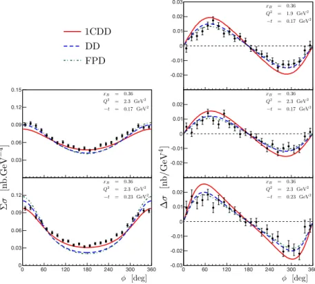
2.3.3 Comparison of a simple model with experimental data . . . 34
2.3.4 Considerations on the D-term . . . 36
2.4 The proton in 1CDD . . . 39
2.4.1 1CDD scheme in the case of a spin-1/2 hadron . . . 39
2.4.2 The D-term as a regulator . . . 40
2.4.3 Comparison to experimental data . . . 43
2.4.4 Beyond this approach . . . 44
3 The Dyson-Schwinger Approach 46 3.1 The Dyson-Schwinger equations . . . 46
3.1.2 Pion Bethe-Salpeter equation . . . 48
3.1.3 Existing truncation schemes . . . 50
3.1.4 Numerical solutions and analytic parameterisations . . . 53
3.1.5 An algebraic model . . . 54
3.2 Mellin moments of the pion GPD . . . 55
3.2.1 Isospin properties . . . 55
3.2.2 The triangle diagram approximation . . . 56
3.2.3 Computing Mellin Moments . . . 58
3.2.4 Comparison with experimental data . . . 61
3.3 From Mellin moments to Double Distributions . . . 63
3.3.1 Polynomial reconstruction and numerical instability . . . 63
3.3.2 Tensorial structure of Mellin Moments and identification with Double Distributions . . . 65
3.3.3 Full reconstruction of the GPD . . . 68
3.3.4 Limitations . . . 71
4 Unravelling gluon ladders 74 4.1 Soft pion theorem . . . 74
4.1.1 Consequences of Axial Vector Ward Takahashi Identity . . . 74
4.1.2 Recovering the soft pion theorem . . . 75
4.2 Forward case . . . 79
4.2.1 Additional contributions to the triangle diagram . . . 79
4.2.2 Double Distribution Computations . . . 81
4.2.3 Limitations in the off-forward case . . . 83
4.3 Sketching the pion 3D structure . . . 84
4.3.1 Correlations between x and t . . . 84
4.3.2 Pion 3D structure . . . 85
5 The overlap representation 88 5.1 GPDs as an overlap of wave functions . . . 88
5.1.1 Lightcone computations . . . 88
5.1.2 Modeling the pion Lightcone Wave Function . . . 92
5.1.3 Distributions on the lightcone . . . 93
5.2 Radon Inverse transformation . . . 96
5.2.1 Problem statement . . . 96
5.2.2 Derivation of the inverse transform . . . 96
5.2.3 A simple example . . . 99
5.2.4 Perspective on the lightcone . . . 104
Conclusion 105
A Conventions and Notations 107
B Euclidean time vs. Minkowskian time 109
C Relation between Γ and ¯Γ 111
E Light front formalism 115
Chapter 1
Introduction to Generalised Parton
Distributions
«L’expérience nous apprend que lorsqu’on entend sonner à la porte, c’est qu’il n’y a jamais personne.» Eugène Ionesco in La cantatrice chauve
1.1 From a point-like proton to Wigner Distributions
1.1.1 The parton model
Discovered in 1919 by E. Rutherford [8], the proton was first thought to be a point-like particle. One has to wait until 1933 to get the first experimental hint for the proton structure [9, 10], through the measurement of its magnetic moment. Due to the Dirac equation, the expected value of the magnetic moment of the proton seen as a point-like particle was:
µp = µN =
e�
2M, (1.1)
were e is the proton charge, M the proton mass, and µN the so-called nuclear magneton.
The results was about 2.5 times greater than expected, a first hint that the proton is not an elementary particle, but a composite one.
This was confirmed 23 years later by Hofstadter through elastic scattering of electrons on nucleons [11]. The amplitude Melof the considered process shown on figure 1.1 can be written
as: Mel= e 2 q2u(k¯ �)γ µu(k)�p 2| Jµem(0)|p1� , (1.2)
where the momenta are defined on figure 1.1 and the matrix element �p2| Jµem(0)|p1� is
pa-rameterised as: �p2| Jµem(0)|p1� = ¯u(p2) � γµF1(q2) + iσµνqν F2(q2) 2M � u(p1) (1.3)
for a spin-1/2 target. F1(q2)and F2(q2) are called form factors and are normalised as:
q2=−Q2
e− e−
p1 p2
k k′
Figure 1.1: Left-hand side: elastic scattering of an electron on a proton target. Right-hand side: original measurement of the proton form factors by Hofstadter (figure from Ref. [12]). with Q being the electric charge and κ the anomalous magnetic moment of the considered hadronic target. It is possible to show that in the case of a point-like target, those form factors do not depend on the photon virtuality Q2. But this is not the case, as measured by
Hofstadter (figure 1.1), definitely proving that the proton is an extended particle.
The following decade was very rich in terms of ideas of what the constituents of the proton (and other hadrons discovered in between) can be. In 1964, M. Gell-Mann [13] and G. Zweig [14, 15] introduced independently a new quantum number called flavour, in order to explain the diversity of hadrons using a SU(3) symmetry. The particles carrying this quantum number were called quarks and thought to be mathematical representations rather than true particles. This status changed at the end of the 1960s with the first Deep Inelastic Scattering (DIS) experiment at SLAC [16, 17].
Indeed, the same year, Björken [18, 19] and Feynman [20] shed some light on the DIS measurements by suggesting that the proton was composed of point-like particles of spin 1/2. This so-called “parton model” was in good agreement with the SLAC results. Its main features are sketched below. Defining the photon virtuality as Q2 =−q2 and P the momentum of the
considered hadron (see figure 1.2), it is possible to write the cross section in terms of the so-called leptonic �µν and hadronic W
µν tensors: d2σ d2ΩdE� = α2 Q4 E� E�µνW µν, (1.5) where α = e2
4π, Ω is the solid angle of the outgoing electrons, E� is the energy of the outgoing
electron and E the energy of the incoming one. This is illustrated on figure 1.2. The leptonic tensor being described only with QED, it can be computed at tree level as:
�µν= 2 � kµk�ν+ k�µkν −Q 2 2 g µν � . (1.6)
where gµν is the metric tensor, kµ and k�µ are respectively the momenta of the incoming
and outgoing electron. The hadronic tensor cannot be directly computed a priori. However, hermiticity and current conservation imply that:
�
Wµν = Wνµ
Thus, assuming the proton target is unpolarised, the hadronic tensor can be parameterised in terms of two structure function F1 and F2:
Wµν(q, P ) =−F1 M � gµν−q µqν q2 � + F2 M P· q � Pµ−P· q q2 q µ � � Pν−P· q q2 q ν � . (1.8)
γ
∗ electron proton k k′ Pγ
∗ electron P xP q xP + qFigure 1.2: Left-hand side: Feynman Diagram of DIS. Right-hand side: interpretation within the parton model. Only the outgoing electron is detected in this process.
Within the parton model, the two functions F1 and F2 can actually be computed. To do
so, it is necessary to introduce the so-called Bjorken variable xB:
xB =
Q2
2P· q. (1.9)
Denoting x the fraction of the proton momentum carried by the active quark (see figure 1.2), they are given as:
F1 =
1
2δ(x− xB), (1.10)
F2 = xδ(x− xB). (1.11)
Introducing the probability density qi(x)to find a given charged parton of type i carrying the
momentum fraction x, and averaging the structure functions, one gets: F1(xB) = � i � dxe2 iqi(x) 1 2δ(x− xB), (1.12) F2(xB) = � i � dxe2 iqi(x) x δ(x− xB). (1.13)
The qi are called Parton Distribution Functions (PDFs). Equations (1.12) and (1.13) have
important consequences, as F1(xB) and F2(xB) are measurable. First, the fact that they do
not depend on Q2 is a direct consequence of the assumption that hadrons are composed of
point-like particles. This is known as Björken scaling. In addition, the Dirac distribution allows one to access experimentally the probability density with respect to xB of those
point-like particles. Moreover, assuming they are spin-1/2 fermions implies the famous Callan-Gross relation [21]:
The experimental agreement of both the Björken scaling1 and the Callan-Gross relation
strongly suggested in those days that the proton was composed of point-like particle of spin 1/2, forty years after the discovery of the proton itself by E. Rutherford.
1.1.2 QCD enters the game
The first DIS experiments were done in a feverish atmosphere around the internal structure of hadrons. After the quark model, it was suggested first that quarks do not obey neither to Bose nor to Fermi statistics [22], and then to add an additional quantum number to quarks called colour in order to explain the structure of the Δ++ in terms of fermionic quarks [23–
25]. The authors also raised the possibility that quarks interact between themselves through eight gauge bosons. Indeed, despite the seminal paper by Yang and Mills in the 1950s [26], it was unclear in those days that strong interaction could be described using a quantum field theory. Light was shed on this in 1973 by Politzer [5] and by Gross and Wilczek [6, 7] who proved that non-abelian gauge theory are asymptotically free. Consequently, one can perform computations in a perturbative framework within a non-abelian gauge theory and thus, take into account the colour degrees of freedom: Quantum Chromodynamics (QCD) was born [27]. Within such a consistent framework for perturbative QCD, leading order (LO) and next-to-leading order (NLO) contributions to DIS were computed. The former give back the results of the parton model, especially equations (1.12) and (1.13). But computations at NLO break both the Björken scaling and the Callan-Gross relation. Predictions for the Q2 dependence
leads to the so-called DGLAP equations [28–30], allowing one to evolve the PDFs at any scale Q2 from an original one Q20. This scaling violation is illustrated on figure 1.3.
Yet until now, a key point was omitted, as one can wonder whether or not it is truly possible in QCD to split the DIS cross section between on one hand a short-range interaction between a charged parton and the incoming photon, and on the other hand a probability density containing all the infrared physics. In other words, whether or not it is possible to write the structure functions as:
F1(xB, Q2) = � i � 1 0 dx C (i) 1 (x, xB, Q2, µ2R, µF2) qi(x, µ2R, µ2F) + O( M2 Q2), (1.15) F2(xB, Q2) = � i � 1 0 dx C(i) 2 (x, xB, Q2, µ2R, µF2) qi(x, µ2R, µ2F) + O( M2 Q2), (1.16)
where C1 and C2 are coefficient functions and do not depend of the considered hadron. M is
the hadron mass, and µR and µF are the so-called renormalisation and factorisation scales.
The coefficient functions depend on those two scales, which indicates that they have been “cured” from divergencies both in the IR and UV sectors. Still, as structure functions are measurable, the dependencies in µF and µR have to cancel out between the PDFs qi and the
coefficient functions C(i)
1 and C (i)
2 . In the parton model, the fact that soft and hard part
factorise comes from the assumption of incoherence between long- and short-distance effects. Proving that this is still true in QCD remains technical and a detailed proof is beyond the scope of this thesis. However, it is possible to give a taste of how things work. Full proofs can be found in original papers [32–35] or in textbooks [36, 37].
1The agreement of experimental data with the Björken scaling in the first DIS data is a coincidence. Indeed
data were taken in a xB-range were the scale dependence is small, and thus cannot be seen because of the
Q2(GeV2) F2 (x,Q 2) * 2 i x H1+ZEUS BCDMS E665 NMC SLAC 10-3 10-2 10-1 1 10 102 103 104 105 106 107 10-1 1 10 102 103 104 105 106
Figure 1.3: The structure function F2 measured at different facilities as a function of Q2,
illustrating the Björken scaling violation. Figure taken from PDG [31].
Before starting, it must be noted that instead of dealing with the hadronic tensor Wµν, it
is easier to focus on the Compton tensor Tµν (figure 1.4) defined as:
Tµν = i 2π � dx4eiq·x1 2 � σ �p, σ| T [Jemµ (x)Jemν (0)]|p, σ� . (1.17)
where T denotes the time ordered products, σ the polarisation of the considered hadron and p its momentum. The Compton tensor is related to the hadronic tensor through the optical theorem:
Wµν= 1 M�[T
µν], (1.18)
where 1/M is merely a normalising factor2, consistently with equation (1.8). One of the
advantages of the Compton tensor is that there are no final-state interactions. Indeed, in figure 1.4 only one jet is allowed in the final state of the Compton tensor. On the opposite, in the case of the hadron tensor (see figure 1.2), multiple jets are allowed, generating soft interactions between them. When trying to factorise the Compton tensor, the first important point is to analyse the large Q2behaviour of the considered process and to show that there is a
one-to-one correspondence with infrared (IR) divergences in massless perturbation theory (see e.g. [36] for an example on the Sudakov form factor). Then one needs to analyse those types of divergences and realises that they correspond to pinch singularities in momentum space. It is therefore possible to define Pinch Singularity Surfaces (PSS) for any considered graph. PSS can be identified through the Landau equations [39], and their contributions can be
interpreted as relativistic on-shell particles in the Coleman-Norton picture [40]. This picture is often represented in terms of so-called reduced graphs. After that, power counting [35, 41] allows the identification of the leading contribution among the reduced graphs. The leading contribution for DIS is shown on figure 1.4, gluons being included in the Wilson lines [42]. The hard part H drawn on figure 1.4 includes all the high virtuality momenta contributions, i.e. k2 ≈ Q2. Finally, a diagrammatic study of the possible values of x shows that the
contributions for x /∈ [−1, 1] vanish, due to poles being in the same half-space of the complex plan. Negative x being interpreted as antiquarks, it is possible to restrict oneself to x ∈ [0, 1], exactly as in the parton model.
Tµν
H
q(x)
xP xP
P P
Figure 1.4: Compton Tensor. Left-hand side: Representation of the Compton tensor. Right-hand side: reduced graph of the leading PSS after including gluons in the Wilson line. H denotes the hard part where momenta have a virtuality of order Q2, whereas q(x) is the PDF.
Within this framework, PDFs can be defined as the Fourier transform of a non-local matrix element: q(x) = 1 2 � dz− 2π e ixP+z− �P | ¯ψq�−z 2 � γ+�−z 2; z 2 � ψq�z 2 � |P ���� z+=z ⊥=0 , (1.19)
where [z1; z2]is the Wilson line between the points z1 and z2 along the lightcone (LC).
Light-cone (LC) variables are defined in appendix A. If DIS is the Golden channel to access PDFs, factorisation theorem allows one to describe different experimental processes. This universal-ity property is a key point in modern hadron and particule physics, as PDFs may be measured in a given process, and used in other ones. They are key elements of physics at colliders, especially at the Large Hadron Collider (LHC). Indeed, computations are done in terms of quarks and gluons but collisions happened between protons. Being the probability density to find a given parton carrying a momentum fraction x inside a hadron, PDFs bridge this gap between fundamental degrees of freedom and observable ones. It should be noted however that within this formulation, there is no direct experimental access to PDFs anymore. Indeed, the structure functions F1 and F2 defined respectively in equations (1.15) and (1.16) give an
experimental access only to convolutions of PDFs with hard scattering kernels. This is why PDF extractions techniques have been developed, see e.g. [43].
To conclude on DIS, one should add that PDFs give a one-dimensional information on the internal structure of the considered hadron. Yet, it is possible to generalise this concept to a multidimensional information and finally build an object which looks like probability densities in kinetic theory: the Wigner Distribution.
1.1.3 Wigner Distributions
Non-relativistic case
In 1932, E. Wigner [44] suggested a generalisation of the phase space distribution f(r, p, t) in the framework of non-relativistic quantum mechanics. Denoting ψ the wave function of the considered particle, the Wigner Distribution is defined as:
W (r, p) = � d3R (2π�)3e−i p·R � ψ∗ � r−1 2R � ψ � r +1 2R � , (1.20)
where bold letters correspond to 3-vectors. The Wigner distribution cannot be seen as a propability density as it contains information on interference, and thus is not positive definite. Yet, in the classical limit, the Wigner distribution becomes positive definite and reduces to the phase-space probability density. However, even in the quantum case, it is possible to compute the expectation value of an operator ˆO(ˆr, ˆp)by convolution with the Wigner distribution [45] (see also Ref. [46]) using the Weyl association rule [47], i.e. associating with a function of r and p denoted OWeyl(r, p):
� ˆO� = �
d3pd3rW (r, p)O
Weyl(r, p). (1.21)
It is also possible to get a probabilistic interpretation for projections of the Wigner distribution: �
d3pW ((r, p) = ρ(r) , � d3rW ((r, p) = ρ(p). (1.22)
Relativistic case
It is possible to extend the notion of Wigner distribution within a a relativistic framework, i.e. using quantum field theory. Introducing gauge invariant quark fields Ψ:
Ψ(x) = exp � −ig � ∞ 0 dλ n · A(λn + x) � ψ(x), (1.23)
where n is a constant four-vector, g the coupling constant and ψ(x) a free quark field, the Wigner operator ˆWΓ is defined as [48, 49]:
ˆ WΓ(r, k+, k⊥) = � dz− d2z ⊥ ei(k +z−−k ⊥z⊥) � ¯ Ψ(r−z 2)ΓΨ(r + z 2) � z+=0, (1.24) where Γ stands for the relevant Dirac structure. ˆWΓ(r, k+, k⊥) is already considered at equal
lightcone time z+ = 0i.e. integrated over k−. The expectation value of this operator within
a hadron gives the Wigner distribution of quarks inside this hadron: WΓ(r, k+,k⊥) = 2M1 � d 3q (2π)3 � H; q 2 � � � ˆWΓ(r, k+,k⊥) � � �H; − q2� = 1 2M � d3q (2π)3e−iq· r�H; q 2 � � � ˆWΓ(0, k+,k⊥) � � �H; − q2�, (1.25) where M is the mass of the considered hadron. Integrating over k⊥ and r would get back the
If Wigner distributions have been originately introduced as six-dimensional objects, they do not correspond to any straightforward physical interpretation. Indeed, relativistic corrections (see e.g. Ref. [50]) preclude interpretations. A five-dimensional definition of the Wigner distri-butions has been given in Ref. [51], allowing a direct interpretation in the Infinite Momentum Frame (IMF). Five-dimensional Wigner Distributions are related to Generalised Transverse Momentum Distributions (GTMDs) through a Fourier transform on coordinate variables in the transverse plane.
Within the past decade, Wigner Distributions and GTMDs have been intensively studied in order to understand the orbital momenta of quarks and gluons inside hadrons (see e.g. [51–58]). Carrying information on both the momenta and the positions of partons, Wigner Distributions are indeed an appropriate object to study orbital momentum. Models of GT-MDs based on lightcone constituent quark model, chiral quark soliton model or light-front wave functions have been developed [54, 57, 58], allowing one to visualise the distribution of transverse momentum.
It does remain unclear whether or not some observables could be directly sensitive to Wigner Distributions in hadron physics. However, today several processes allow to get an experimental access to projections of the Wigner Distributions. DIS is one of them but brings only a one-dimensional information on the hadron structure through PDFs. Nonetheless, it is nowadays possible to do better, for instance through exclusive processes.
1.2 Exclusive processes
1.2.1 Exclusive vs Inclusive
Contrary to inclusive processes like DIS, exclusive processes require to characterise every particles in the final state. They are therefore much harder to measure than inclusive ones. However they also contain much more information. Three different processes are considered here, with three particles in the final state. Deep Virtual Compton Scattering (DVCS) in which a lepton interacts with a hadron through the exchange of a virtual photon. A photon is detected in the final state together with the lepton and the hadron (figure 1.5). A crossed process can be identified in which a real photon interacts with the hadron, producing a virtual photon which decays into a lepton pair. This process is called Time-like Compton Scattering (TCS) and is illustrated on figure 1.5. A third process called Deep Virtual meson production (DVMP) contains three particles in the final state. This process is similar to DVCS except that in the final state, a meson is produced instead of a real photon.
γ∗ ℓ′ ℓ P−Δ 2 P + Δ 2 γ γ∗ ℓ′ ℓ P−Δ 2 P + Δ 2 γ
1.2.2 Factorisation and Generalised Parton Distributions
Just as in DIS, the question of the possibility to describe exclusive processes as convolutions of a hard part computed using QCD perturbative expansion, and a soft part encoding the non-perturbative information can be raised. In the case of DIS, the proof of this factorisation is already very technical. Dealing with exclusive processes, things do not simplify. Indeed, exclusive processes cannot be factorised at the level of the cross section, but at the level of the amplitude. It is then possible to apply the same machinery than for the DIS case, i.e. identify the PSS and select the relevant ones using power counting [59–61]. But other techniques have been developed in order to factorise the DVCS amplitude like for instance the one based on the Operator Product Expansion (OPE) done by the Leipzig group [62]. A third one consists in writing a general graph contribution to the process in the Schwinger α-representation and identifying within this framework the leading contributions in Q2 [63–66].
All those methods show that it is indeed possible to factorise the DVCS (and also TCS and DVMP) amplitude into a hard part expandable within a perturbation theory framework and a soft part containing the non-perturbative information. Actually, the previous mentioned proofs of factorisation naturally lead to different objects encoding the non-perturbative behaviour. Dealing with PSS leads to the Generalised Parton Distributions (GPDs) (see for instance Ref. [60]) Hq and Eq which are defined in terms of matrix elements as:
Fq = 1 2 � dz− 2π e ixP+z− �p2| ¯ψq � −z 2 � γ+ψq�z 2 � |p1� � � � z+=z ⊥=0 = 1 2P+ � Hq(x, ξ, t)¯u (p2) γ+u (p1) + Eq(x, ξ, t)¯u (p2) iσ+µΔµ 2M u (p1) � , (1.26) where P = p1+p2
2 and Δ = p2− p1. x is the average fraction of the momentum of the active
quark along the hadron direction, ξ = −Δ+
2P+ is the boost along the same direction as shown on the left-hand side of figure 1.6. t = Δ2 is the Mandelstam variable, and q stands for the
quark flavour. Two additional quark GPDs ˜H and ˜E can be introduced in the very same way: ˜ Fq = 1 2 � dz− 2π e ixP+z− �p2| ¯ψq � −z2�γ+γ5ψq�z 2 � |p1� � � � z+=z ⊥=0 = 1 2P+ � ˜ Hq(x, ξ, t)¯u (p2) γ+γ5u (p1) + ˜Eq(x, ξ, t)¯u (p2) γ5Δ+ 2M u (p1) � . (1.27) In addition to quark GPDs, gluon GPDs can be defined:
Fg = 1 P+ � dz− 2π e ixP+z− �p2| G+µ � −z2�Gµ+�z 2 � |p1� � � � z+=z ⊥=0 = 1 2P+ � Hg(x, ξ, t)¯u (p2) γ+u (p1) + Eg(x, ξ, t)¯u (p2) iσ+µΔ µ 2M u (p1) � , (1.28) ˜ Fg = 1 2 � dz− 2π e ixP+z− �p2| G+µ � −z 2 � ˜ Gµ+�z 2 � |p1� � � � z+=z ⊥=0 = 1 2P+ � ˜ Hg(x, ξ, t)¯u (p2) γ+γ5u (p1) + ˜Eg(x, ξ, t)¯u (p2)γ5Δ + 2M u (p1) � , (1.29) where Gµν is the gluon field strength and ˜Gµν = 1
2�µνρσGρσ. If gluon GPDs do not play
non-perturbative object, called Distribution Amplitude (DA), which describes the probability amplitude to create a meson, given the momentum fractions of the two quarks. This is illustrated on figure 1.6 −q2= Q2 q′ e−(k) p1= P−Δ2 p2= P +Δ2 GPDs e−(k− q) (x + ξ)P+ (x− ξ)P+ p1= P−Δ2 p2= P + Δ 2 GPDs DA −q2= Q2
Figure 1.6: Left-hand side: One of the LO contribution of the quark GPDs to the DVCS amplitude. Right-hand side: One of the LO contribution of the gluon GPDs to the DVMP amplitude.
Equations (1.26), (1.27), (1.28) and (1.29) are relevant to define GPDs related to spin-1/2 hadrons. However, a significant part of the present work is devoted to the pion, whose relevant GPDs are defined as:
Hπq(x, ξ, t) = 1 2 � dz− 2π e ixP+z− �p2| ¯ψq � −z 2 � γ+ψq�z 2 � |p1� � � � z+=z ⊥=0 (1.30) Hπg(x, ξ, t) = 1 P+ � dz− 2π e ixP+z− �p2| G+µ � −z2�Gµ+�z 2 � |p1� � � � z+=z ⊥=0 . (1.31) The equivalents of ˜Hq and ˜Hg have to vanish due to discrete symmetries.
The Schwinger α-representation does not lead directly to GPDs, but rather to the so-called Double Distributions (DDs). Of course, as the same physics is described by those two non-perturbative objects there is a way to go from one to the other. The discussion on DDs and their relation to GPDs is left for chapter 2.
1.3 Generalised Parton Distributions: Properties
1.3.1 Support, continuity and interpretation
Just like in the case of PDFs, it is possible to perform an analysis of the analytic properties of the matrix elements defining the GPDs, and thus to deduce properties of GPDs themselves. In the lightcone gauge where A+= 0, the GPD H can be viewed as the projection of a off-shell
parton-hadron scattering amplitude: H(x, ξ, t) = 1 2 � dk+d2k ⊥δ � x− k + P+ � � dk−A(k) (1.32) with: A(k) = � d4zeik·z � P + Δ 2 � � � � T � ¯ ψ�−z 2 � γ+ψ�z 2 �� ��� �P − Δ 2 � , (1.33)
T denoting time ordering. Following the arguments of Ref. [67], A depends on the following variables: t (fixed by the kinematics), s =�P −Δ2 − k1�2, u =�P + Δ2 + k1�2, k21 = (k−Δ2)2
and k2
2 = (k + Δ2)2. As done for instance in Ref. [67–69], we assume here that the analytic
properties of the non-perturbative amplitude coincides with the ones given by a perturbative analysis through Feynman graphs. Therefore, cuts are expected in the s and u channel for non-negative �(s) and �(u), singularities for non-negative �(k2
1) and �(k22). Usually, those
singularities are taken into account by adding a −i� term, shifting them slightly below the real axis. In the case of equation (1.32), doing so regularise the integral over k− and the amplitude
A(k).
k1 k2
p1 p2
Figure 1.7: GPD as an off-shell scattering amplitude. As previously, p1 = P −Δ2 and p2 =
P + Δ2.
In order to locate singularities of A(k) in the complex k− plane, one can write k− as:
s = � P−Δ 2 − k1 �2 → k−= s + (k⊥) 2 2P+(x− 1)+ P− (1.34) u = � P +Δ 2 + k1 �2 → k−= u + (k⊥) 2 2P+(x + 1)+ P− (1.35) k12= (k−Δ 2) 2 → k−= k 2 1+ � k⊥−Δ⊥ 2 �2 2(x + ξ)P+ + Δ 2 − (1.36) k22= (k + Δ 2) 2 → k−= k 2 2+ � k⊥+Δ⊥ 2 �2 2(x− ξ)P+ − Δ 2 − . (1.37)
Due to the regularisation, poles and cuts of A(k) have now imaginary parts proportional to −i�. For instance, a pole originally located at k2
2 = q2 is now shifted at q2 − i�. Fixing ξ
such as ξ ∈ [−1, 1], it is possible to locate the singularities in the complex plan with respect to the value of x. Indeed, the previous denominators change sign for x = 1, x = −1, x = −ξ and x = ξ. Consequently, it appears that for |x| > 1, all the possible singularities are in the same half-part of the complex plane (below the real axis), and thus one can close the integration contour without including any singularities, as shown on figure 1.8. Therefore, providing that A vanishes sufficiently fast at infinity, the GPD is zero for |x| > 1. Then for all the different regions delimited by the change of signs in the denominators, looking carefully at the integration contour, it is possible to show that using or not using the time-ordered product leads to the same results [67].
Concerning the GPDs themselves (equation (1.26)) it is interesting to see what is going on when Δ = 0, i.e. when the incoming and outgoing protons carry the same momenta:
Hq(x, 0, 0)u(P )γ¯ +u(P ) 2P+ = 1 2 � dz− 2π e ixP+z− �P | ¯ψq�−z 2 � γ+ψq�z 2 � |P ���� z+=z ⊥=0 . (1.38)
Im k Re k-- Im k Re k
-Figure 1.8: Momentum complexe plane integration. Left-hand side: x > 1; all poles and cuts are below the real axis, allowing integration around the upper half plan and leading to a vanishing GPD. Right-hand side: −1 < x < 1; poles and cuts are spread in the entire plane, leading to a non vanishing GPD.
As ¯u(P )γ+u(P ) = 2P+ in the infinit momentum frame, one realises that this matrix element
is the one defining PDFs (equation (1.19)) and thus that:
Hq(x, 0, 0) = q(x) for x ≥ 0, (1.39)
Hq(x, 0, 0) = −¯q(−x) for x ≤ 0. (1.40)
In addition to the PDFs, GPDs also contain the quark contribution to the form factors F1 and
F2 defined in equation (1.3). For a spin-1/2 targets, integrating the GPDs H and E leads to:
� 1 −1dx H q(x, ξ, t) = Fq 1(t) , � 1 −1dx E q(x, ξ, t) = Fq 2(t). (1.41)
Another interesting analytic property is the continuity at the point x = ξ. Continuity is required for the sake of factorisation. Indeed, if the GPDs were not continuous, logarithmic divergences would arise when computing observables (see section 1.4 for details). Therefore, consistency requires the GPDs to be continuous at x = ξ. The points x = ±ξ also play an important role in terms of the interpretation. Indeed, as shown on figure 1.9 for the quark GPD, one can see the virtual photon interacting with a quark (ξ ≤ x ≤ 1), with an anti-quark (−1 ≤ x ≤ −ξ) or with quark anti-quark pair (−ξ ≤ x ≤ ξ) [70–73].
ξ − x −x − ξ −1≤ x ≤ −ξ x +ξ ξ − x −ξ ≤ x ≤ ξ x +ξ x − ξ ξ ≤ x ≤ 1
Figure 1.9: Different interpretations depending on the relative value of x and ξ respectively.
1.3.2 Mellin moments and symmetries
Discrete symmetries generate interesting GPD properties. In particular time reversal invari-ance constrains the GPDs to be even in ξ:
The same relations can be found for ˜Hq, ˜Eq, Hg, Eg, ˜Hg and ˜Eg. This is expected as
time reversal interchanges the initial and final states, i.e. interchanges the momenta in the definition of Δ and thus of ξ = p+2−p+1
p+2+p+1 leading to a additional minus sign. Details are given in
appendix D. Another important point concerns the consequences of hermiticity. Taking the hermitian conjugate of the non-local matrix element (1.26) leads to:
[H(x, ξ, t)]∗ = H(x,−ξ, t) , [E(x, ξ, t)]∗= E(x,−ξ, t), (1.43) which together with the time reversal results (1.42) force the GPDs to be real.
Beyond the form factors, it is also possible to relates higher Mellin moments Mm(ξ, t)
defined as:
Mm(ξ, t) =
� 1 −1dx x
mH(x, ξ, t), (1.44)
to local operators. Indeed, integrating the local matrix element of equation (1.26) in the lightcone gauge yields:
� dx xm1 2 � dz− 2π e ixP+z− �p2| ¯ψq � −z 2 � γ+ψq�z 2 � |p1� � � � z+=z ⊥=0 = 1 2(iP+)m � dz− 2π ∂m ∂z−m �� dx eixP+z−� �p2| ¯ψq � −z 2 � γ+ψq�z 2 � |p1� � � � z+=z ⊥=0 = 1 2(iP+)m+1 � dz− ∂m ∂z−m � δ�z−���p2| ¯ψq � −z 2 � γ+ψq�z 2 � |p1� � � � z+=z ⊥=0 = 1 2(P+)m+1�p2| ¯ψ q(0) γ+�i←∂→+�mψq(0)|p 1� , (1.45) where ←→∂ + = −→∂+−←−∂+
2 . In other gauges than the lightcone one, the gauge link generates
a covariant derivative ←D→ instead of a partial one. Equation (1.45) also suggests to define a typical operator:
O{µµ1...µm} = ¯ψγ{µi←D→µ1...i←→Dµm}ψ (1.46) with {...} meaning that the operator is taken completely symmetrised and that the traces are removed. Defining the twist τ as the difference between the dimension d in mass units and the spin s:
τ = d− s, (1.47)
O{µµ1...µm} is the twist-two operator of spin m. Within the Wilson OPE formalism [74] those local operators appear in the Taylor expansion of the non-local one along the lightcone [62, 75].
They can be parameterised as: �p2| O{µµ1...µm}|p1� = ¯u(p2)γ{µu(p1) [m 2] � i=0 Aqm+1,2i(t) � −Δ 2 µ1� ... � −Δ 2 µ2i� Pµ2i+1...Pµm} +¯u(p2) σ{µαΔα 2M u(p1) [m 2] � i=0 Bm+1,2iq (t)Δµ1...Δµ2iPµ2i+1...Pµm} −mod(2, m)¯u(p2)Δ {µ 2Mu(p1)C q m+1(t) � −Δ 2 µ1� ... � −Δ 2 µm}� , (1.48)
where the even powers of ξ are selected by the time reversal invariance. mod(2, m) vanishes if m is even, and is 1 if m is odd, [ · ] is the floor function. As ξ = −Δ·n
2P·n, it is straitforward
to see that those local matrix elements are polynomials in ξ. Considering the Gordon identity relating the different Dirac structure among them, one gets:
� dx xmH(x, ξ, t) = [m 2] � j=0 ξ2jAqm+1,2i(t) +mod(m, 2)ξm+1Cm+1q (t), (1.49) � dx xmE(x, ξ, t) = [m 2] � j=0 ξ2jBm+1,2iq (t)− mod(m, 2)ξm+1Cm+1q (t). (1.50) This is the famous polynomiality property of the GPDs. The Aq, Bq and Cq are sometimes
called generalised form factors. The polynomiality property comes from the decomposition of the local matrix elements (1.48) in terms of those generalised form factors. This decomposition encodes the Lorentz symmetry and so does the polynomiality property.
It is worth stressing that being given a full set of Mellin moments, it is possible to associate it to a unique function f providing that f is continuous on a segment. This is a consequence of the Stone-Weierstraß theorem. Thus it is possible to recover the original function from the Mellin moments.
1.3.3 Positivity
If polynomiality is a key property of GPDs coming from Lorentz invariance, the positivity property comes directly from wave function considerations and the Cauchy-Schwartz inequal-ity. Indeed, considering the scalar case at t = 0, the GPD H can be described as:
H(x, ξ) =�
S
�Ψout(x, ξ, S)| Ψin(x, ξ, S)�, (1.51)
where Ψin(x, ξ, S) is the probability amplitude that the considered hadron splits in a quark
carrying a x+ξ momentum fraction along the average direction P+, and a spectator S. In the
same way, Ψout(x, ξ, S)is the probability density that a quark with a momentum fraction x−ξ
recombines with the spectator S to give back the considered hadron. This decomposition of the GPDs in terms of wave functions has been derived in the lightcone quantisation framework [72] (see appendix E) and is detailed in chapter 5. From equation (1.51), applying the Cauchy-Schwarz inequality, one gets [76]:
� � � � � � S �Ψout(x, ξ, S)| Ψin(x, ξ, S)� � � � � � 2 ≤� S �Ψout(x, ξ, S)| Ψout(x, ξ, S)� � S� � Ψin(x, ξ, S�)�� Ψin(x, ξ, S�)�. (1.52)
Defining the variables x1 and x2 as:
x1 = x− ξ 1− ξ = k2+ p+2 , x2 = x + ξ 1 + ξ = k1+ p+1 , (1.53)
which are the momentum fractions of the quark interacting with respectively the outgoing and incoming hadrons, it is possible to identify the PDFs:
� S �Ψout(x, ξ, S)| Ψout(x, ξ, S)� = q(x1), (1.54) � S� � Ψin(x, ξ, S�)�� Ψin(x, ξ, S�)� = q(x2). (1.55)
This leads to the following inequality between GPDs and PDFs:
Hq(x, ξ)≤�q(x1)q(x2). (1.56)
An equivalent inequality can be derived for gluon distributions: Hg(x, ξ)≤�(1− ξ2)x
1x2g(x1)g(x2). (1.57)
Those results are neither limited to the scalar case nor to the GPD H, and can be extended to other hadrons and other GPDs [72, 77, 78] or to the so-called impact parameter space GPDs [79].
Both polynomiality and positivity are fundamental properties of the Generalised Parton Distributions, and thus must be fulfilled in order to expect agreement on ξ-dependent ob-servables. If different ways of modeling GPDs ensure automatically either polynomiality (see chapter 2) or positivity (see chapter 5), it remains hard to fulfil both at the same time [80, 81], despite attempts to create a framework ensuring both properties [82]. However it must be added that one type of Ansatz for the wave function allows to fulfil both [83, 84].
1.3.4 Evolution
Just like PDFs, GPDs depend on renormalisation and factorisation scales. The behaviour of GPDs with respect to the factorisation scale can be perturbatively computed at a given order. In this framework, quark and gluon GPDs a priori mix between each other. But it is possible to introduce linear combinations allowing one to deal with decoupled equations. Decoupled linear combinations are called non-singlet (NS), whereas coupled combinations are called singlet. One of the NS term can be defined as:
FN Sq (x, ξ, t) = Fq(x, ξ, t) + Fq(−x, ξ, t), (1.58) which is also called the valence GPD due to its limit in the forward case. Such a combination has a fixed C-parity in the t-channel. In this case, C = −1, i.e. in the t-channel, exchanges have C = −1 parity. Evolving this combination, no C = 1 exchanges can be added. Moreover, as gluons are their own anti-particles, gluon GPDs have a C = 1 parity and thus they cannot be mixed with NS combinations. Due to the non-mixing with gluons, the NS GPDs obey an autonomous evolution equation:
µ2F ∂ ∂µ2 F FN S(x, ξ, t) = � dy 1 |ξ|KN S � x ξ, y ξ � FN S(y, ξ, t), (1.59)
where KN S is called the NS evolution kernel.
Contrary to the NS case, the so-called singlet case defined as: �
q
�
has a C = 1 parity in the t-channel, and thus gluon GPDs enter the computation of the singlet kernels through the exchange of two gluons in the t-channel producing a quark anti-quark pair. In order to deal with this mixing of quark and gluon contributions in the evolution kernel, it is convenient to introduce the vector F :
F = � (2nf)−1�qFq(x, ξ, t)− Fq(−x, ξ, t) Fg(x, ξ, t) � , (1.61)
where nf stand for the number of active flavour, and which fulfils a equation similar to equation
(1.59) with a kernel K: K = K qq�x ξ, y ξ � Kqg�xξ,yξ� Kgq�x ξ, y ξ � Kgg�x ξ, y ξ � . (1.62)
The evolution kernels KN S and K can be computed perturbatively and are known at LO
[62, 66, 85–92] and at NLO [93–97].
As it has been seen before in equations (1.39) and (1.40), GPDs reduce to PDFs in the forward limit (i.e. ξ → 0). Consistently, the off-forward evolution kernels KN S and K also
reduce to the NS and singlet DGLAP kernels respectively. When ξ → 1, the off-forward evolution kernels reduce to other well-known quantities. Indeed, one gets back the famous ERBL kernels [98–102] which describe the evolution of DAs. DAs will be introduced in further details in chapter 2.
Solving those equations is crucial for phenomenological applications. To proceed, one can either choose a numerical approach and use algorithms based for instance on Runge-Kutta methods, like the author of Ref. [103]. Or it is also possible to try through OPE to diagonalise those equations. This method is a classical way to evolve PDFs, as their Mellin moments qm(µF)are directly related to local twist-two operators:
qm(µF) =
�
dx xmq(x, µ
F) = nµnµ1· · · nµm�P | O{µµ1···µm}|P � . (1.63) Using the fact that the structure function F1(x, Q) defined at equation (1.15) is observable,
and thus neither itself nor its Mellin moments depend on µF, one gets the following differential
equation:
µFdµd F
ln (qm(µF)) =−γm(αs(µ2F)) (1.64)
in the non-singlet case. αs is the strong coupling constant and γm is the NS anomalous
dimension. The singlet case is similar, and details can be found for instance in Ref. [37]. The operators O{µµ1···µm} do not mix with each other and support multiplicative renormal-isation. Therefore, Mellin moments of PDFs evolve independently from each other within a multiplicative framework from the scale µ0
F to µ1F: qm(µ1F) = qm(µ0F) exp −12� 2 ln � µ1F µ0F � 0 dtγ m�αs�(µ0F)2et �� . (1.65)
The same approach can be used for GPDs, but using different local operators and thus different moments. Indeed, as soon as ξ �= 0, GPD Mellin moments mix themselves through evolution equations. The same mixing problem has been stressed even for simpler objects like
DAs [98, 100–102]. But in this case, it has been proved that at LO, evolution equations can be diagonalised providing that one considers the so-called twist-two conformal operators:
Omq = (∂+)mψ¯qγ+Cm3/2 �−→D+−←D−+ − → ∂++←−∂+ � ψq, (1.66) where C3/2
m is the 32-Gegenbauer polynomial of degree m. It should be noticed that the
derivative at the denominators cancel with the one in front of the expression, leading to a well-defined expression. The importance of conformal moments here is not a coincidence. Indeed, the QCD Lagrangian fulfils conformal symmetry at a classical level. Consequently, the fact that the evolution equations are diagonalised on a basis of conformal operators testifies the presence of conformal symmetry. However, conformal symmetry is broken by quantisation. As quantum fluctuations introduce UV divergences, an intrinsic scale, the renormalisation scale and a renormalisation condition are needed to properly define the theory. The coupling constant varies with this scale, breaking the conformal symmetry. Thus, when taking into account quantum fluctuations, the multiplicative renormalisation of the conformal operators (1.66) have to break down at some point. This is the case at NLO, as they start mixing with each others.
Those arguments of conformal theory are detailed for instance in Ref. [69, 104] and can also be applied to GPDs. Indeed, defining GPDs conformal moments Cq
m(ξ, t)as: Cmq(ξ, t) = ξm � 1 −1dx C 3/2 m � x ξ � Hq(xξ, t) (1.67)
for quarks, and as:
Cmg(ξ, t) = ξm−1 � 1 −1dx C 5/2 m−1 � x ξ � Hg(xξ, t) (1.68)
for gluons, they diagonalise the evolution equations of GPDs at LO.
1.3.5 Hadron 3D tomography
Just like PDFs, GPDs can be seen as projections of Wigner Distributions. Indeed, integrating equation (1.25) over k⊥ leads to:
� d2k ⊥ (2π)2Wγ+(r, k +,k ⊥) = 1 2M � d3q (2π)3e−iq·r � dz−eik+z− � q 2 � � � ¯ψ�−z 2 � γ+ψ�z 2 � ���−q 2 ���� z+=z ⊥=0 , (1.69) which is the Fourier transform of the GPDs (up to an overall factor) for q = Δ. This suggests that GPDs are related to quark and gluon multidimensional probability densities. But as stressed already for Wigner Distributions, GPDs are not positive definite and thus the prob-abilistic interpretation is not straightforward. However, as it has been shown in Ref. [50], it is possible to get a true probabilistic interpretation at ξ = 0. More precisely, defining:
ρq(x,b⊥) =� d 2Δ ⊥ (2π)2e−ib⊥ Δ⊥Hq(x, 0,−Δ2 ⊥), (1.70)
ρq(x,b
⊥) can be seen as the probability density to find a quark of flavour q carrying a given
fraction x of the hadron momentum along the lightcone, and at a given position b⊥ in the
transverse plane to this lightcone direction. An example of probability density is shown on figure 1.10. 0. 0.5 1 � 0.5 0. 0.5 b�M 0. 0.5 1. 1.5 2. q �x, b�� M2 x
Figure 1.10: Transverse plane density of the pion GPD. 3D-plot of ρq(x,b
⊥) coming from
Ref. [105].
1.4 GPD extraction
Focusing on the DVCS process, one can split the full Compton amplitude in eight contributions coming from the different quark and gluon GPDs. Those contributions are called Compton Form Factors (CFF) and are convolutions of the different GPDs with their respective hard parts. More explicitly, denoting F the CFF:
F(i)(ξ, t) = � 1
−1dx C
(i)(x, ξ)F(i)(x, ξ, t), (1.71)
where (i) denotes the different types of GPDs F(i) of quarks and gluons. C(i) stands for the
hard part associated with the GPD F(i)and depending on the considered process.
Dependen-cies in Q2, renormalisation and factorisation scales of GPDs and hard parts are omitted here
for brevity. Focusing on the GPD H, one can write its associated CFF H at LO as: H(ξ, t) = � 1 −1dx � 1 ξ− x − i�− 1 ξ + x− i� � H(x, ξ, t). (1.72)
Due to the singularities at x = ±ξ, the CFF H(ξ, t) is a complex number. It is possible to relate its real and imaginary parts to the GPD as:
� (H(ξ, t))|LO = p.v. � 1 −1dx � 1 ξ− x− 1 ξ + x � H(x, ξ, t), (1.73) � (H(ξ, t))|LO = π (H(ξ, ξ, t)− H(−ξ, ξ, t)) , (1.74)
where p.v stand for the Cauchy principal value prescription. It should also be noticed that at LO, gluons do not play any role in the DVCS amplitude and therefore Cg
LO = ˜CLOg = 0.
Contrary to the DIS case where the PDFs are accessible directly at LO (see equations (1.12) and (1.13)), only the line x = ξ of the entire GPDs phase space is directly accessible at LO through the imaginary part of the CFF H. The real part is already a convolution.
Nonetheless, the extraction of the CFFs themselves is challenging. Considering the four GPDs previously introduced, one has a priori eight quantities to extract (real and imaginary parts). Yet, existing dispersion relations between real and imaginary parts of the CFFs reduce this number to four. Still, it remains a hard task as few data are actually available. Extraction techniques have been developed in order to fit CFFs to available data using least square minimisation. Two approaches can be highlighted: a local fit which considers CFFs as free parameters [106] and a global fit which parameterises the CFFs through a generic functional form of the GPD [107–109]. The former method has the advantage to be model-independent apart from the twist-two approximation, but is hardly suitable for extrapolation and hard to interpret. The latter can be extrapolated providing a suitable parameterisation, but carries an intrinsic model-dependence through the functional parameterisation. A third pioneering way is actually explored, which consists in extracting the CFFs using neural networks [110].
In addition to the difficulty of extracting CFFs, one should keep in mind that, just like in the case of DIS and PDFs, the interpretation of data in terms of GPDs becomes even harder at NLO. NLO corrections for DVCS are now well-known [111–117] and their effects are truly significant on CFFs [118]. One of the possible explanations is the role played by the gluon GPDs which do not appear at LO (see figure 1.11) and bring brand new contributions rather than a correction to the leading one. The importance of the gluon effects in the DVCS has motivated people to resum higher-order contributions. This has been done in the quark sector [119], and is still an ongoing work in the gluon sector. Resummation is also important due to the possible dependence of the CFF on the factorisation scale at NLO. The selection of the relevant factorisation scale and the understanding of such a dependence on CFF remain open questions. γ∗ γ P−Δ 2 P + Δ 2 GPDs P−Δ2 P + Δ 2 GPDs γ∗ γ
Figure 1.11: Example of possible NLO corrections. Left-hand side: quark GPD contribution. Right-hand side: gluon GPD contribution.
Data interpretation can also be challenged by the so-called target mass corrections. Indeed, the interpretation requires Q2 to be large compared to any other energy scale of the process.
Yet, as shown on figure 1.13, the current available DVCS data have been taken for values of Q2 � 2 GeV2, except for H
1 and ZEUS data. Compared to the proton mass M2 � 1 GeV2,
the ratio between those two mass scales is not that small, generating correction depending on M2/Q2 (or t/Q2). If this point was well-known for DIS [120, 121], those kind of corrections
have been computed only recently for exclusive processes [122, 123]. In the case of DVCS, the correction are significant, as shown in recent study [124] and illustrated on figure 1.12
Figure 1.12: Effect of target mass corrections on DVCS unpolarised cross sections [124]. The model KM10a has been developed is the one of Ref. [108], and the target mass corrections derived in Ref. [122, 123] have been computed thanks to the KMS model of Ref. [125].
Several sets of data have been produced in the last 15 years both in fixed target and collider configurations. Collider results probe the small-xB region as shown on figure 1.13,
whereas fixed target experiments probe large to medium values of xB. Among the latter,
the HERMES collaboration has provided the community with asymmetries varying both the beam polarisation and the target polarisation. Within normalised notations [125], ABT stands
for the asymmetry measured with a beam polarisation B and a target polarisation T. The HERMES collaboration was able to measure all the independent DVCS observables, except cross-sections (see e.g. [126, 127] for a exhaustive description of the available data). DVCS cross-sections have been measured at Jefferson Laboratory (JLab), and published by the Hall-A [129] and CLHall-AS [130] collaborations in addition to asymmetries measured by the CLHall-AS collaboration [131]. Moreover, a recent reanalysis of the Hall-A data [124] suggests that target mass corrections are important when dealing with JLab kinematics.
Concerning future experiments, on a short time scale the upgrade of JLab from 6 GeV to 12 GeV energy beam should increase significantly both the kinematic range of available data and their precision, challenging our understanding of nucleon structure. On a longer time scale, an Electron-Ion Collider (EIC) should fill the gap between the current and future fixed target experiments, and the small-x data obtained by the ZEUS and H1 collaborations.
Q2=100 GeV2
Q2=50 GeV2
Planned DVCS at fixed targ.:
COMPASS- dσ/dt, ACSU, ACST
JLAB12- dσ/dt, ALU, AUL, ALL Current DVCS data at colliders:
ZEUS- total xsec
ZEUS- dσ/dt H1- total xsecH1- dσ/dt H1- ACU Current DVCS data at fixed targets:
HERMES- ALT HERMES- ACU HERMES- ALU, AUL, ALL HERMES- AUT Hall A- CFFs CLAS- ALU CLAS- AUL 1 10 102 103 10-4 10-3 10-2 10-1 1 x Q 2 (GeV 2 ) EIC √s= 140 GeV, 0.01 ≤ y ≤ 0.95 y ≤ 0.6 y ≤ 0.6 EIC √s= 45 GeV, 0.01 ≤ y ≤ 0.95
Figure 1.13: Existing DVCS measurement and planned experiements. Figure from EIC white paper [128].
Chapter 2
The Double Distributions Approach
«To succeed, planning alone is insufficient.One must improvise as well.» Isaac Asimov in Fundation.
2.1 Definitions and properties
As mentioned in section 1.2.2, when factorising exclusive processes, Generalised Parton Dis-tributions are not the only way to parameterise the considered non-local matrix elements. The α parameterisation leads to another non-perturbative object called Double Distributions (DDs). Introduced at the same time as GPDs1 [62, 65, 66, 132], they encode the information
contained in a non-local matrix element as: � P + Δ 2 � � � � ¯q � −z2�γµq�z 2 � ��� �P −Δ2����� z2=0 = 2Pµ � Ω dβdα e−iβ(P·z)+iα(Δ2·z)Fq(β, α, t) −Δµ � Ω dβdα e−iβ(P·z)+iα(Δ2·z)Gq(β, α, t)
+higher twist terms, (2.1)
for a scalar hadron. Fq(β, α, t)and Gq(β, α, t) denote the two quark DDs. The analphabetic
order of variables α and β follows the convention of Ref. [133]. Historically, the DD Gq(β, α, t)
was first overlooked, then introduced under a specific form in Ref. [134] and generalised in Ref. [135]. Equivalent relations can be introduced for the different operators introduced in section 1.2.2, defining the corresponding DDs. In the case of a spin-1/2 hadron, the additional
Lorentz structure leads to an additional DD denoted Kq(β, α, t): � P +Δ 2 � � � � ¯q � −z2�γµq�z 2 � ��� �P − Δ 2 ���� � z2=0 = ¯u � P +Δ 2 � � γµ � Ω dβdα e−iβ(P·z)+iα(Δ2·z)Fq(β, α, t) +iσµνΔ ν 2M � Ω dβdα e−iβ(P·z)+iα(Δ2·z)Kq(β, α, t) −Δµ 2M � Ω dβdα e−iβ(P·z)+iα(Δ2·z)Gq(β, α, t) � ×u � P −Δ 2 �
+ higher twist terms. (2.2) As shown on figure 2.1, both variable β and α have an interpretation in terms of parton and hadron momenta. In the forward case, i.e. Δ = 0, the variable β can be directly identified with the PDF momentum fraction x. On the other hand, when P = 0 the diagram on figure 2.1 looks like the one of a DA, allowing one to relate α with a DA parameter.
βP− (1 + α)Δ 2 βP + (1− α)Δ2 P−Δ 2 P + Δ 2
Figure 2.1: Momenta associated with hadrons and partons within a DD framework. The α variable plays also an important role in terms of discrete symmetries. Indeed the analysis of time reversal invariance detailed in appendix D leads to definite parities in α for the DDs Fq(β, α, t), Kq(β, α, t) and Gq(β, α, t), as it was the case for the GPDs in terms of
the variable ξ (equation (1.42). More precisely one gets: �
Fq(β,−α, t) = Fq(β, α, t)
Kq(β,−α, t) = Kq(β, α, t) , G
q(β,−α, t) = −Gq(β, α, t). (2.3)
The Double Distributions depend on two adimensional variables juste like in the case of the GPDs and those variables live on a compact support Ω. The latter is defined by the following constraint:
Ω ={(β, α), |β| + |α| ≤ 1} , (2.4)
and is illustrated on figure 2.2. The proof of the DDs’ support property is achieved using the α-representation of Feynman diagrams (see e.g. Ref. [66]).
Encoding the non-perturbative information contained in an exclusive process, DDs depend on a factorisation scale µR. Consequently, they obey evolution equations [62, 65, 66, 132]
similar to equation (1.59). And once again, it is possible to define singlet and non-singlet sectors. In the present work, the choice has been done to evolve GPDs rather than DDs (the relation between the two is given in the next section).
Figure 2.2: The rhombus defining the support of the Double Distributions in the (β, α) plane.
2.2 Recovering GPDs
2.2.1 Radon transform and operator product expansion
GPDs and DDs are Fourier transforms of the same operator. However, GPDs are single-dimensional Fourier transforms with respect to the variable z− (1.26) assuming that P · z
and Δ · z are proportional to each other through the kinematics parameter ξ. Therefore, GPDs depend both on x, the conjugate variable of z−, and ξ. On the other hand, DDs are
two-dimensional Fourier transforms (equations (2.1) and (2.2)) of the considered light-front operator. Within the DD framework, P · z and Δ · z are considered as independent and their Fourier conjugate variables are denoted β and α. Consequently the DDs do not depend on the kinematic parameter ξ. In the scalar case, the relation between GPDs and DDs comes from: Hq(x, ξ, t) = 1 2 � dz− 2π e ixP+z− �p2| ¯ψq � −z 2 � γ+ψq�z 2 � |p1� � � � z+=z ⊥=0 = 1 2 � dz− 2π e ixP+z− 2P+ � Ω dβdα e−iβ(P+z−)+iα(Δ+z−)2 (Fq(β, α, t) + ξGq(β, α, t)) = � Ω dβdα (Fq(β, α, t) + ξGq(β, α, t))� dz− 2π P +eiP+z−(x−β−αξ) = � Ω dβdα (Fq(β, α, t) + ξGq(β, α, t)) δ(x− β − αξ). (2.5) The GPDs are therefore convolutions of the DDs with a Dirac δ. In a more geometrical point of view, the GPD Hq(x, ξ, t) correspond of the DDs F (β, α, t) and G(β, α, t) integrated
along a line of equation x − β − ξα = 0 in the (β, α) plane. Mathematically, this kind of relation between two functions is known as the Radon Transform [136], and has revealed itself extremely convenient for tomography [137]. Considering a function f, its Radon transform R [f] is given by:
R [f] (s, φ) = �
du dv f(u, v)δ(u cos(φ) + v sin(φ) − s). (2.6) In the language of GPDs, x = s
cos(φ) and ξ = tan(φ). Mathematically, the Radon transform
can be inverted, and thus it would be in principle possible to get back the Double Distributions from the GPDs. However, numerically inverting the Radon transform reveals itself technical in the case of GPDs. Consequently, the discussion on inversion of the equation (2.5) is left for


![Figure 1.12: Effect of target mass corrections on DVCS unpolarised cross sections [124]](https://thumb-eu.123doks.com/thumbv2/123doknet/14663123.740149/29.892.155.754.222.462/figure-effect-target-corrections-dvcs-unpolarised-cross-sections.webp)
![Figure 1.13: Existing DVCS measurement and planned experiements. Figure from EIC white paper [128].](https://thumb-eu.123doks.com/thumbv2/123doknet/14663123.740149/30.892.193.718.415.796/figure-existing-dvcs-measurement-planned-experiements-figure-white.webp)