HAL Id: hal-00815502
https://hal.archives-ouvertes.fr/hal-00815502
Submitted on 18 Oct 2013
HAL is a multi-disciplinary open access
archive for the deposit and dissemination of
sci-entific research documents, whether they are
pub-lished or not. The documents may come from
teaching and research institutions in France or
abroad, or from public or private research centers.
L’archive ouverte pluridisciplinaire HAL, est
destinée au dépôt et à la diffusion de documents
scientifiques de niveau recherche, publiés ou non,
émanant des établissements d’enseignement et de
recherche français ou étrangers, des laboratoires
publics ou privés.
Simulation of Real-Time Multiprocessor Scheduling with
Overheads
Maxime Chéramy, Anne-Marie Déplanche, Pierre-Emmanuel Hladik
To cite this version:
Maxime Chéramy, Anne-Marie Déplanche, Pierre-Emmanuel Hladik. Simulation of Real-Time
Multi-processor Scheduling with Overheads. International Conference on Simulation and Modeling
Method-ologies, Technologies and Applications (SIMULTECH 2013), Jul 2013, Reykjavik, Iceland. pp. 5-14.
�hal-00815502�
Simulation of Real-Time Multiprocessor Scheduling with Overheads
Maxime Ch´eramy
1,2, Anne-Marie D´eplanche
3and Pierre-Emmanuel Hladik
1,21CNRS, LAAS, 7 avenue du colonel Roche, F-31400 Toulouse, France 2Univ de Toulouse, INSA, LAAS, F-31400 Toulouse, France
3LUNAM Universit´e - Universit´e de Nantes, IRCCyN UMR CNRS 6597, (Institut de Recherche en Communications et
Cybern´etique de Nantes), ECN, 1 rue de la Noe, BP92101, F-44321 Nantes cedex 3, France {maxime.cheramy, pehladik}@laas.fr, [email protected]
Keywords: real-time, scheduling, simulation, multiprocessor, overheads, cache
Abstract: Numerous scheduling algorithms were and still are designed in order to handle multiprocessor architectures, raising new issues due to the complexity of such architectures. Moreover, evaluating them is difficult without a real and complex implementation. Thus, this paper presents a tool that intends to facilitate the study of schedulers by providing an easy way of prototyping. Compared to the other scheduling simulators, this tool takes into account the impact of the caches through statistical models and includes direct overheads such as context switches and scheduling decisions.
1
INTRODUCTION
The study of real-time scheduling had regained inter-est this last decade with the continuous introduction of multiprocessor architectures. Multiple approaches have been used to handle those architectures (Davis and Burns, 2011). A first approach, called partition-ing, consists of splitting the task set into subsets. Each of these subsets is allocated to a unique processor on which a mono-processor scheduler is then run. In contrast, a second approach, called global schedul-ing, allows tasks to migrate from processor to proces-sor. In that case, there is a single queue of ready tasks and a single scheduler for all the processors. Finally, as a compromise that aims to alleviate limitations of partitioned (limited achievable processor utilization) and global (non-negligible overheads) algorithms, hy-brid policies such as semi-partitioned and clustered scheduling have been proposed more recently (Bas-toni et al., 2011).
By far the greatest focus on multiprocessor real-time scheduling has been put on algorithmic and theo-retical issues. Indeed, for the various scheduling poli-cies, a lot of attention has been paid to define analyti-cal schedulability tests. However, those results rely on general and simple models of the considered software and hardware architectures quite far away from the practical ones. Such research must now address im-plementation concerns as well. Actually, multiproces-sor architectures bring more complexity with shared
caches and memory, new communication buses, inter-processor interrupts, etc. They also raise new imple-mentation issues at the operating system level: which core should run the scheduler?, what data should be locked?, etc.
Thus, new scheduling policies that try to take ben-efits from the specificities of the hardware architec-ture (such as the caches) must be designed and tools for studying them must be made available. One way for this is to use a cycle-accurate simulator or even a real multiprocessor platform, and to execute real tasks. In that case, the results are very accurate, how-ever it requires developing the scheduler in a low-level language and integrating it into an operating sys-tem. This work can potentially take a lot of time. Fur-thermore, the generation of various and realistic tasks for a massive evaluation is laborious.
In consequence, it is preferable to use an “intermediate-grained” simulator able to simulate with a certain level of accuracy the behavior of those (hardware and software) elements that act upon the performances of the system. Such a simulator allows fast prototyping and does not require a real implemen-tation of the tasks nor the operating system. More-over, extensive experiments can be easily conducted and various metrics are available for analysis. Its in-trinsic drawback is that it will never reflect exactly how a scheduler behaves in details on a real system but it should be enough to give good insights on gen-eral tendencies.
Our contribution is a simulation tool, called SimSo (“SImulation of Multiprocessor Scheduling with Overheads”), that is designed to be easy to use and able to take into account the specificities of the system, starting with LRU caches, context-save/load overheads and scheduling overhead. SimSo1 is an open source tool, actively developed, designed to fa-cilitate the study of the behavior of schedulers for a class of task systems and a given hardware architec-ture. For that, we propose to extend the Liu and Lay-land model (Liu and LayLay-land, 1973) to bring enough information to characterize how the tasks access the memory. This allows us to use statistical models to calculate the cache miss rates and to deduce job exe-cution times. Moreover, our simulator has been con-ceived as flexible as possible to be able to integrate other task and architecture models.
This paper is organized as follows. First, we ex-plain our motivation in section 2. The main principles of real-time scheduling are explained in section 3. Then we explain how the simulator has been imple-mented in section 4. Section 5 presents the scheduler component and section 6 deals with the integration of the hardware models. We present the simulation soft-ware in section 7 and we compare it to the existing similar tools in section 8. To conclude, we summa-rize our contribution and present our future works in section 9.
2
MOTIVATION
Most of the multiprocessor real-time scheduling strategies have been designed without taking into ac-count the presence of caches and their effects on the system behavior. Though, interferences on the cache of preempted and preempting tasks allocated to the same processor may cause additional delays (Mogul and Borg, 1991). In the same way, when a cache is shared by multiple processors, the execution of a task can have a significant impact on another task running on another processor. Furthermore, schedul-ing overheads and context switch overheads are often regarded as negligible. However, on a multiproces-sor system, schedulers tend to generate more preemp-tions, more migrations and even more rescheduling points in order to achieve a high utilization of the pro-cessors (Devi and Anderson, 2005).
Significant research effort has been focused on the problem of real-time multiprocessor scheduling since the late 1990’s, in particular in the area of global scheduling. It led to a number of optimal
al-1Available at http://homepages.laas.fr/mcheramy/simso/.
gorithms (PFair and its variants PD and PD2, ERFair, BF, SA, LLREF, LRE-TL, etc.) that are very attrac-tive because theoretically able to correctly schedule all feasible task sets without processing capacity un-used (Davis and Burns, 2011). However their prac-tical use can be problematic due to the potentially excessive overheads they cause by frequent schedul-ing decisions, preemptions and migrations. There-fore, being able to take them into account helps in the predictability analysis of such real-time systems for which the first requirement is to meet time constraints. Moreover, reducing the overall execution time of the tasks can also bring significant benefits (for instance, better response times or less power consumption).
Following these observations, recent research has emerged and new scheduling algorithms appeared which aim to reduce the overheads by bounding the amount of preemptions (Bastoni et al., 2011; Nelis-sen et al., 2012). Also, a few studies have shown that avoiding co-scheduling tasks that heavily use a shared cache can reduce the overall execution time (Fedorova et al., 2006; Anderson et al., 2006). Finally, other re-searches focus on cache space isolation techniques to avoid cache contention on shared caches (Guan et al., 2009; Berna and Puaut, 2012).
Our primary objective is the comparison of those numerous scheduling policies and their associated variants. Currently, the only way to compare them is by far to try to put in relation the properties exhib-ited by their authors: computational complexity, num-ber of scheduling points, utilization bound, numnum-ber of task preemptions, number of task migrations. Such a task is quite intractable since evaluations have been made under separate conditions. Instead our intention is to make available a framework allowing to study as precisely as possible the performance of a scheduler and to establish relevant comparisons between dif-ferent scheduling policies based on the same bench-marks. For instance, given a system correctly schedu-lable with multiple scheduling policies, we would like to pick the one that should be the most efficient (less overhead). For that, we would aim to identify general trends for classes of tasks and hardware architectures. A typical result could be: scheduler A is better than B in most cases, except when the shared cache is too small given the characteristics of the tasks.
We expect from these results to help the real-time community to better understand the cache effects on scheduling, and bring new ideas that could help to conceive schedulers which take benefits from the caches.
3
CONTEXT
In this part, we briefly present the context of real-time multiprocessor scheduling and its relevant models in order to facilitate the understanding of the following. This also precises a few assumptions made for the simulation.
A real-time application is composed of tasks, i.e. programs, to be run on a hardware architecture made of a limited number of processors. Real-time means that the computing of tasks has to meet time con-straints (typically release times and deadlines). The scheduler is a software system component whose pur-pose is to decide at what time and on which processors tasks should execute. Therefore, a real-time sched-uler takes its decisions according to the urgency of the tasks.
Tasks The model most commonly used to describe the tasks is the Liu and Layland one (Liu and Layland, 1973). In this model, a great abstraction is made since a task is simply viewed as a computation time. This means that its functional behavior is ignored as it will be discussed in section 6. In our simulation, when the caches are taken into consideration, some extra parameters are necessary as explained in 6.2.1.
A task can be respectively periodic, sporadic, or aperiodic depending on its inter-activation delay, re-spectively constant, minimum, or unknown. A task activation gives rise to the release of a job (an instance of the task) that must complete before a given dead-line date.
The tasks neither share memory nor communicate between each other but precedence relations between tasks may be specified so that the activation of an ape-riodic task follows the end of another task.
Processors We consider symmetric multiprocess-ing hardware architectures (SMP) which are the most common multiprocessor design nowadays. In such architecture, the processors are identical and share a single main memory. Private and/or shared caches are associated to them in a hierarchical way. The model-ing of the cache hierarchy as well as their time ac-cess costs are given in section 6.2.2. Note that we focus our work on architectures with less than a few dozen processors. Thus, Network On Chip (NoC) ar-chitectures, which present an interest for many-core systems, are not considered.
Scheduler Among the various scheduling strate-gies, one distinguishes time- and event-triggered ones depending on the conditions in which the scheduler is
invoked: a rescheduling has to be made either at spec-ified instants, or when a job completes or a new one is released. In addition, the scheduler may be preemp-tive and decide to interrupt the execution of a job and to resume it later. In the same way, schedulers may allow tasks and their jobs to partly or freely migrate and execute on multiple processors.
4
IMPLEMENTATION
4.1
Discrete-event Simulation
The core of the simulator is implemented using SimPy (SimPy Developer Team, 2012), a process-based discrete-event simulation library for Python. The advantage of a discrete-event simulation over a fixed-step one is that it is possible to handle short du-rations (such as a context-switch overhead) as well as long durations (such as a job execution) with the same computational cost. We have chosen SimPy because it can be easily embedded as part of a software, it is well-documented and easy to use.
According to SimPy’s vocabulary, a Process is an entity that can wait for a signal, a condition or a cer-tain amount of time. When it is not waiting, a Process can execute code, send signals or wake up other pro-cesses. This Process state is called “active”, opposed to “passive”. A Process is activated by another Pro-cessor by the simulation main class itself.
The simulation unit is the processor cycle to al-low a great precision. However, for user convenience, the attributes of the tasks, such as the period or the deadline, are defined in milliseconds (floating-point numbers) and converted in cycles using a parameter named cycles per ms.
4.2
Architecture
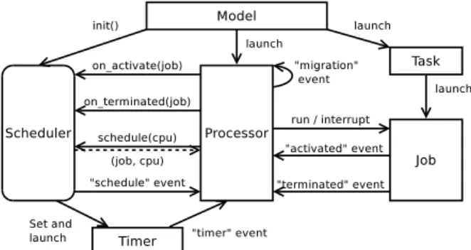
The main classes and their mutual interactions are represented in Figure 1 and described below:
• Model is the simulation entry point, it will instan-tiate and launch the processors and the tasks as active Processes. It will also call the init method of the scheduler so that it can initialize its data structures and launch timers if needed.
• A Task handles the activations of its jobs. The activations are either periodic or triggered by an other task (aperiodic). Depending on a property of the task, the jobs that exceed their deadline can be aborted.
• A Job simulates, from a time-related aspect only, the execution of the task code. Its progression is
Figure 1: Interactions between main class instances. Pro-cessor, Task, Job and Timer are Process objects and can have multiple instances.
computed by the execution time model (see sec-tion 6). A signal is sent to its running processor when it is ready and when its execution is finished. • A Processor is the central part and simulates the behavior of the operating system running on a physical processor. There is one Processor for each physical processor. It controls the state of the jobs (running or waiting) in accordance with the scheduler decisions. It also deals with the events: activation or end of a job, timer timeout, sched-ule request, etc. The attribute “running” of a pro-cessor points to the job that is running (if any). Figure 2 provides a very simplified diagram rep-resenting what a processor does. Similarly, as a real system, some actions can induce overheads (e.g. context switch or scheduling decision) and only affect the concerned processor.
• A Timer allows the execution of a method after a delay, periodically or not. On a real system, this method would run on a physical processor, thereby inducing a context switch overhead if a job were running on the same processor. This be-havior is reproduced by sending a “timer” event to the processor.
• The Scheduler is described in section 5. Unlike the previous elements, the scheduler is not a Pro-cessobject, all its methods except the init method are called by the Processor objects.
5
SCHEDULER COMPONENT
5.1
Scheduler Interface
In order to implement a scheduler, the user has to de-velop a class that inherits from the abstract Scheduler class. The scheduler interface is partly inspired by
Figure 2: Simplified execution workflow of a Processor. The “terminated” event is a particular event that will not cause a context save overhead.
what can be found on real operating systems such as Linux but kept as simple as possible. This interface allowed us to develop partitioned, global and hybrid schedulers. The scheduler interface is shown in Fig-ure 1.
When the simulation is started, the init method is called. It is then possible to initialize data structures and set timers if required. When the scheduler needs to make a scheduling decision, it sends a “schedule” event to the processor that will execute the schedule method. This event is sent as a consequence of a job activation, termination or through a timer. This lets the possibility to write schedulers that are either time-driven, event-driven or both. The processor is in charge of applying the scheduling decision (which includes an inter-processor interrupt if needed).
5.2
Handling Various Kinds of
Scheduling
In order to deal with multiprocessor scheduling, vari-ous strategies are possible: a global scheduler for all the processors, a scheduler for each processor, or even intermediate solutions. The support of any kind of scheduler is done at a user level.
Take a partitioned scheduling as an illustration of this, we define a “virtual” scheduler that will be in-stantiated by the simulation and called by the proces-sors. This scheduler will then instantiate one mono-processor scheduler for each mono-processor and allocate each task to one scheduler. The links between the processors and the schedulers as well as the links be-tween the tasks and the schedulers are saved. Thus, when a processor calls a method of the “virtual” scheduler, the latter retrieves the concerned scheduler and forwards the method call to it.
By generalizing this example by allocating one scheduler to any number of processors and by allow-ing a task to migrate from one scheduler to another,
we see that any kind of scheduling is feasible. Thus, this approach has the advantage of being very flexible. Moreover, we provide a few examples to guide.
5.3
Lock
For global or hybrid strategies, some scheduler vari-ables (such as the list of ready tasks) are shared be-tween the processors. As a consequence, a protection mechanism can be required to avoid inconsistencies. Such protections form a bottleneck which induces ex-tra overheads.
A mechanism of lock is provided by the simulator in order to reproduce these overheads. This lock is intended to prevent to run the scheduler at the same simulation time on two or more different processors. The developer of a scheduler can decide to deactivate the lock by overriding the get lock method.
5.4
Example
In this section, we present what a user could de-velop to simulate a global EDF. The source code is in Python.
A detailed explanation of this example is available in the documentation of the tool. Instead we would like to draw the reader’s attention on the small number of lines required. An actual implementation of this policy in an operating system would require hundreds of lines.
from core import Scheduler class G_EDF(Scheduler):
"""Global Earliest Deadline First""" def init(self):
self.ready_list = [] def on_activate(self, job):
self.ready_list.append(job)
# Send a "schedule" event to the processor. job.cpu.resched()
def on_terminated(self, job):
# Send a "schedule" event to the processor. job.cpu.resched()
def schedule(self, cpu): decision = None # No change. if len(self.ready_list) > 0:
# Get a free processor or the processor run-# ning the job with the latest deadline. key = lambda x: (1 if not x.running else 0,
x.running.absolute_deadline if x.running else 0)
cpu_min = max(self.processors, key=key)
# Get the job with the highest priority # within the ready list.
job = min(self.ready_list,
key=lambda x: x.absolute_deadline) # If the selected job has a higher priority # than the one running on the selected cpu: if (cpu_min.running is None or (cpu_min.running.absolute_deadline > job.absolute_deadline)): self.ready_list.remove(job) if cpu_min.running: self.ready_list.append(cpu_min.running) # Schedule job on cpu_min.
decision = (job, cpu_min) return decision
6
JOB COMPUTATION TIME
6.1
A Generic Approach
Generally, scheduling simulation tools consider only the worst-case execution time (WCET) for the execu-tion time of the jobs. Depending on the tool, the user may also have the possibility to configure the simu-lator to use the average-case execution time (ACET) or a random duration between the best-case execution time (BCET) and the WCET.
One of our objectives is to take into consideration the impact of the memory accesses on the computa-tion time in order to be as accurate as possible. A sig-nificant difference with the classical approach is that the total execution time of a job can only be known when it finishes. Indeed, the execution time depends on the scheduling decisions (which tasks were execut-ing on the other processors, was it preempted, etc.).
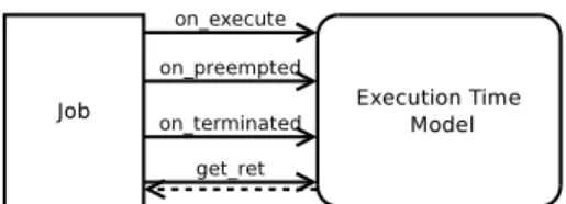
The components needed to compute the execution time are purposely isolated from the rest of the sim-ulator and implement a generic interface to interact with the simulator. As shown in Figure 3, the model receives an event when the state of a job is changed. The job uses the get ret method to get a lower bound of its remaining execution time. While this duration is strictly positive, the job is not finished.
For example, a computation time model based on the WCET is trivial. The get ret method simply re-turns the WCET minus the duration already spent to run the job. The remaining methods of the interface have nothing to do because that duration is given and kept up-to-date by the job itself.
This design is sufficiently generic to easily swap the models used to compute the execution time of the jobs. Hence, alternative models could be developed to
Figure 3: Interface of any execution time model.
simulate a different hardware or to adjust the accuracy of the results.
6.2
Modeling Memory Behaviors
In this section, we briefly present how the impact of the caches is implemented as an execution time model as explained above.
6.2.1 Memory Behavior of a Task
In order to characterize the memory behavior of the tasks, we extended the model of Liu-Layland with ad-ditional information. For each task τ, the user must provide:
• Number of instructions: the average number of instructions executed by a job of τ.
• Base CPI: the average number of cycles required to execute an instruction without considering the memory access penalties (base cpiτ).
• Memory access rate: mixτis defined as the
pro-portion of instructions that access the memory among all.
• Stack distance profile (SDP): the distribution of the stack distances for all the memory accesses of a task τ is the stack distance profile (sd pτ),
where a stack distance is by definition the number of unique cache lines accessed between two con-secutive accesses to a same line (Mattson et al., 1970). An illustration of this distance is provided by Figure 4. Such metric can be captured for both fully-associative and N-way caches (Chan-dra et al., 2005; Babka et al., 2012).
3
1 0 1
t
A B C B B D A D
Figure 4: Memory accesses sequence. A, B, C and D are cache lines and numbers indicate the stack distances.
These information can be automatically generated or retrieved from a real application. The number of instructions, the memory access rate and the stack dis-tance profile can be generated using tools such as an
extension to CacheGrind (Babka et al., 2012), Stat-Stack (Eklov and Hagersten, 2010) or MICA2(Hoste and Eeckhout, 2007). The base CPI requires a cycle accurate simulator. It is the computation time in cy-cles divided by the number of instructions.
6.2.2 Cache Hierarchy
We consider hierarchical cache architectures. A list of caches (e.g. [L1, L2, L3]) can be associated to each processor. Caches can be shared between several processors while it respects the inclusive3property.
A cache is defined by a name, its associativity, its size, and the time needed to reach it (in cycles).
For now, only data caches with Least Recently Used (LRU) as replacement policy is considered, the generalization to instruction caches is left for future work. Hence, a few modifications in the cache de-scription are likely to occur in order to make the dis-tinctions between instruction caches, data caches and unified caches.
6.2.3 Cache Models
Depending on which tasks are running in concurrency and the initial state of the caches, the execution speed of the jobs varies.
The goal of the cache models is to determine, on a given time interval, the average number of cycles per instructions (CPI) of a job, taking into consideration the impact of the various tasks on the caches. Using the CPI, it is then possible to determine the number of instructions executed by a job during that interval.
The duration returned by the get ret method (see Figure 3) is simply the time required to execute the re-maining number of instructions if the job was running alone on the system without any interruption.
Cache sharing induces two kinds of extra cache misses:
• Following a preemption: a job may have lost its cache affinity when another job is running on the same processor. Some of the evicted lines should then be reloaded.
• Shared between multiple processors: two or more tasks that are simultaneously running on differ-ent processors with a shared cache, do not tend to share this cache equally.
For the first case, we have taken the simplifying assumption that the cache filling follows an
exponen-2MICA does not generate complete SDP so we had to
patch it.
3Caches are inclusives if any data contained in a level of
tial distribution and we use the SDP of the task to de-termine the number of lines that should be reloaded. However, other models exist (Liu et al., 2008) and we are also currently working on better estimations of the cache loading using Markov chains.
For the second case, we used the FOA model (Chandra et al., 2005) that has fast running times and gives reasonable results according to the authors. Obviously, other models (Eklov et al., 2011; Chandra et al., 2005; Babka et al., 2012) could be im-plemented as well.
The state of the caches (the number of lines for each task) is kept up-to-date at each change in the sys-tem (start, interruption or end of a job).
7
SIMULATION TOOL
7.1
Features
Open source The source code, the documen-tation and the examples are freely available at http://homepages.laas.fr/mcheramy/simso/.
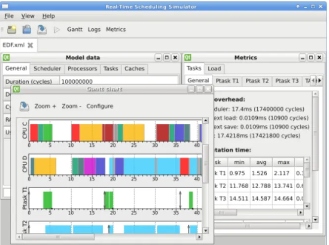
Configuration The user interface of the simulator (Figure 5) provides a straightforward graphical inter-face to load the scheduler class and to define the tasks, the processors, the caches and their hierarchy, and the various parameters for the simulation. The resulting configuration is saved into an XML file. However, such a file could also be generated automatically by an external tool without using the graphical user in-terface. This is important in order to run extensive simulations with auto-generated properties.
Output When the configuration is completed and checked, the user can launch the simulation and ob-tain a Gantt chart representing the result of the sim-ulation or a textual equivalent representation. Some metrics are provided to the user such as the number of preemptions, migrations, the time spent in the sched-uler, the computation time of each job, etc.
Speed and limitations The simulation runs very fast, as an example, simulating a global EDF with 4 processors, 10 tasks, 2 levels of caches for a duration of 100ms (108cycles) takes less than one second on an Intel Core i5. There are no technical limitations on the number of processors but the cache models imple-mented in the present version have not been validated by their authors for a large number of processors.
Figure 5: User interface of the tool showing the simulation of a global EDF.
7.2
Use as an Educational Tool
The user interface of the simulator has been designed keeping in mind it could also be used for an educa-tional purpose. This is the main reason why all the inputs can be set through a graphical user interface and the results displayed in a Gantt chart.
As shown in the previous example, it allows a fast prototyping of schedulers in Python. This lan-guage is easy to learn and yet very powerful and ef-fective (Radenski, 2006).
Regarding the simulation, it is also possible to consider WCETs as effective task computation times. Thus, the input is simpler and more usual.
This tool is already used by Master’s students in a real-time systems course at INSA Toulouse. From an applicative real-time project, students have to model its various tasks and then use the simulator to under-stand how the processors are shared between the tasks using a fixed priority scheduler.
7.3
Application Example
As a reminder, our primary goal is the study of scheduling policies. In the following, we present through a simple case study, how our tool could be used to better understand the real behavior of a sys-tem.
Problem description In this example, we would like to compare the scheduling of a system using the Earliest Deadline First algorithm with a global (G-EDF) and a partitioned (P-(G-EDF) strategy. G-EDF is a generalization of EDF for multiprocessor that uses a single ready task queue whereas P-EDF starts with a definitive allocation of the tasks on the processors
and then runs multiple mono-processor EDF sched-ulers for handling each processor.
Input The eight considered tasks are all periodic4 and synchronous with the start of the simulation. Their SDP was taken from the MiBench bench-mark (Guthaus et al., 2001), the first five tasks are making more accesses to the memory than the last three (according to their value of mix).
For the task partitioning phase (P-EDF only), a WCET for each task is mandatory. WCET values were chosen by bounding with a safety gap the experi-mental times given by the simulation. Table 1 synthe-sizes the period and WCET values of the tasks. Task partitioning was done using the First Fit algorithm. The result of the partitioning is: {T1, T2}, {T3, T4, T5}, {T6, T7}, {T8}.
Table 1: List of tasks (total utilization is 82.5%).
T1 T2 T3 T4 T5 T6 T7 T8
Period (ms) 20 20 15 15 10 10 10 10
WCET (ms) 11 9 7 5 2 6 4 3
The simulated hardware architecture, including four processors and a cache hierarchy, is summa-rized in Figure 6. Each L1-cache is an LRU fully-associative cache of 2KiB (32 lines of 64 bytes). The L2 cache is an LRU fully-associative cache of 16KiB (256 lines of 64 bytes). The second level of cache is relatively small when compared to what can usually be found on modern architectures. This choice is jus-tified by the small memory footprint of the selected benchmarks and the will to show the impact of cache contention through this example.
Figure 6: Simulated hardware architecture. Numbers repre-sent the access time in cycles (10−9s).
The scheduling overhead is set to 0.1ms (100.000 cycles) and a context save or load overhead to 0.0001ms (100 cycles).
The duration of the simulation is ten seconds. Observations Table 2 shows the load using both strategies. The payload corresponds to the time spent executing the tasks (including cache overheads) and the system load is the time wasted in the system
4A periodic task releases a job every period time units.
(scheduler and context-switch overheads). Because of the order of magnitude of a scheduling overhead compared to the overhead of a context save or load, the system load is mostly the time spent waiting for a scheduler decision. The number of scheduling de-cisions remains similar in both cases, however, the global lock required for G-EDF adds an additional overhead. We can assume that this gap in system load between the two strategies will increase with more processors. This is in accordance with the results of Bastoni et al stating that G-EDF is not a viable choice for hard real-time systems with a large number of pro-cessors (24 in their study) (Bastoni et al., 2010).
Table 2: Load for both schedulers. Total load Payload System load G-EDF 72.2 % 68.0 % 4.2 % P-EDF 68.3 % 65.1 % 3.2 %
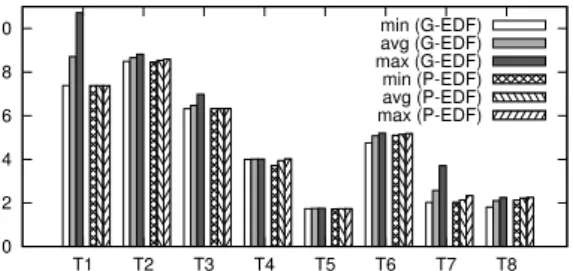
The computation times of the jobs are shorter with P-EDF compared to G-EDF as shown in Figure 7. In proportion to G-EDF, the payload for P-EDF is 4.2% lower in this example. The first reason is that the tasks that use the more the memory are merged in the first two processors, partly avoiding co-scheduling. The second reason is the reduction of the number of pre-emptions (1501 for G-EDF against only 666 for P-EDF) and task migrations (3500 against 0) which led to less cache reloading.
This result seems compatible with the work done by Fedorova et al that shows in their case study an improvement of the system throughput up to 32% for a non-real-time system (Fedorova et al., 2006).
0 2 4 6 8 10 T1 T2 T3 T4 T5 T6 T7 T8 min (G-EDF) avg (G-EDF) max (G-EDF) min (P-EDF) avg (P-EDF) max (P-EDF)
Figure 7: Effective task Computation times.
Obviously, in order to confirm these results, we shall conduct larger studies. Because the duration of a simulation run is very short, it is then possible to run thousands of experiments with different configu-rations. Such complete studies are in progress but out of scope of this paper.
8
RELATED WORK
Most of the work on real-time multiprocessor scheduling addresses the theory only. Davis and Burns give a good insight of the current state of the researches in their survey (Davis and Burns, 2011).
A first approach for considering real-world over-heads in the study of such scheduling policies is to use a cycle-accurate simulator or a real system.
There are two major simulator available. The first one, Gem5 is the merger of the M5 and GEMS simu-lators (Binkert et al., 2011). It simulates a full system with various CPU models and a flexible memory sys-tem that includes caches. The second one, Simics, is a commercial product able to simulate full-systems but it is not cycle-accurate (Magnusson et al., 2002).
LITMUSRT (Calandrino et al., 2006), developed at the University of North Carolina (UNC), offers a different approach. It is not a simulator but an exten-sion of the Linux Kernel which provides an exper-imental platform for applied real-time research and that supports a large number of real-time multipro-cessor schedulers.
With both kind of tools, a substantial investment in time is required to learn how to use them and to write some new scheduler components.
There are also several tools emerging from the academic community and dedicated to the simula-tion of real-time systems such as Cheddar (Singhoff et al., 2004), MAST (Harbour et al., 2001), Storm (Urunuela et al., 2010) and others (Rodr´ıguez-Cayetano, 2011; Chandarli et al., 2012). Most of these tools are designed to validate, test and analyze systems. Storm is probably the most advanced tool focusing on the study of the scheduler itself. However it does not handle direct overheads such as context-switches or scheduling overheads. Nor does it handle the impact of caches.
9
CONCLUSIONS
This paper presents a simulator dedicated to the study of real-time scheduling. It was designed to be easy to use, fast and flexible. Our main contribution, when compared to the existing scheduling simulators, is the integration of overheads linked to the system (context-switching, scheduling decision) and the im-pact of the caches.
We have shown in this paper that it is possible to take the impact of the caches into consideration. However, the models we currently use could proba-bly be replaced by better ones. This replacement can easily be done as explained in section 6. We are
al-ready thinking about new models but they have to be validated using cycle accurate simulators.
Once our cache models will be validated and inte-grated into the simulator, we will launch a large cam-paign of simulations. As a reminder, our long term goal is the classification of the numerous scheduling policies with practical considerations. We hope that it will also help the researchers to spot the weaknesses and the strengths of the various strategies. We would be pleased if our simulation tool could be the source of innovative ideas.
ACKNOWLEDGEMENTS
The work presented in this paper was conducted under the research project RESPECTED (http://anr-respected.laas.fr/) which is supported by the French National Agency for Research (ANR), program ARPEGE.
REFERENCES
Anderson, J., Calandrino, J., and Devi, U. (2006). Real-time scheduling on multicore platforms. In Proc. of the 12th IEEE Real-Time and Embedded Technology and Applications Symposium (RTAS).
Babka, V., Libiˇc, P., Martinec, T., and T˚uma, P. (2012). On the accuracy of cache sharing models. In Proc. of the third joint WOSP/SIPEW International Conference on Performance Engineering (ICPE).
Bastoni, A., Brandenburg, B., and Anderson, J. (2010). An empirical comparison of global, partitioned, and clus-tered multiprocessor edf schedulers. In Proc. of the IEEE 31st Real-Time Systems Symposium (RTSS). Bastoni, A., Brandenburg, B., and Anderson, J. (2011). Is
semi-partitioned scheduling practical? In Proc. of the 23rd Euromicro Conference on Real-Time Systems (ECRTS).
Berna, B. and Puaut, I. (2012). Pdpa: period driven task and cache partitioning algorithm for multi-core systems. In Proc. of the 20th International Conference on Real-Time and Network Systems (RTNS).
Binkert, N., Beckmann, B., Black, G., Reinhardt, S. K., Saidi, A., Basu, A., Hestness, J., Hower, D. R., Kr-ishna, T., Sardashti, S., Sen, R., Sewell, K., Shoaib, M., Vaish, N., Hill, M. D., and Wood, D. A. (2011). The gem5 simulator. SIGARCH Computer Architec-ture News.
Calandrino, J. M., Leontyev, H., Block, A., Devi, U. C., and Anderson, J. H. (2006). LitmusRT: A testbed for em-pirically comparing real-time multiprocessor sched-ulers. In Proc. of the 27th IEEE International Real-Time Systems Symposium (RTSS).
Chandarli, Y., Fauberteau, F., Masson, D., Midonnet, S., and Qamhieh, M. (2012). Yartiss: A tool to visual-ize, test, compare and evaluate real-time scheduling algorithms. In 3rd International Workshop on Analy-sis Tools and Methodologies for Embedded and Real-time Systems (WATERS).
Chandra, D., Guo, F., Kim, S., and Solihin, Y. (2005). Pre-dicting inter-thread cache contention on a chip multi-processor architecture. In Proc. of the 11th Inter-national Symposium on High-Performance Computer Architecture (HPCA).
Davis, R. I. and Burns, A. (2011). A survey of hard real-time scheduling for multiprocessor systems. ACM Computing Surveys, 43(4).
Devi, U. and Anderson, J. (2005). Tardiness bounds under global edf scheduling on a multiprocessor. In Proc. of the 26th IEEE Real-Time Systems Symposium (RTSS). Eklov, D., Black-Schaffer, D., and Hagersten, E. (2011). Fast modeling of shared caches in multicore systems. In Proc. of the 6th International Conference on High Performance and Embedded Architectures and Com-pilers (HiPEAC).
Eklov, D. and Hagersten, E. (2010). StatStack: efficient modeling of LRU caches. In Proc. of the IEEE Inter-national Symposium on Performance Analysis of Sys-tems Software (ISPASS).
Fedorova, A., Seltzer, M., and Smith, M. (2006). Cache-fair thread scheduling for multicore processors. Tech-nical Report TR-17-06, Division of Engineering and Applied Sciences, Harvard University.
Guan, N., Stigge, M., Yi, W., and Yu, G. (2009). Cache-aware scheduling and analysis for multicores. In Proc. of the 7th ACM international conference on Embedded Software (EMSOFT).
Guthaus, M., Ringenberg, J., Ernst, D., Austin, T., Mudge, T., and Brown, R. (2001). Mibench: A free, commer-cially representative embedded benchmark suite. In Proc. of the IEEE International Workshop on Work-load Characterization (WWC-4).
Harbour, M. G., Garc´ıa, J. J. G., Guti´errez, J. C. P., and Moyano, J. M. D. (2001). Mast: Modeling and analysis suite for real time applications. In Proc. of the 13th Euromicro Conference on Real-Time Systems (ECRTS).
Hoste, K. and Eeckhout, L. (2007). Microarchitecture-independent workload characterization. Micro, IEEE, 27(3).
Liu, C. L. and Layland, J. (1973). Scheduling algorithms for multiprogramming in a hard-real-time environment. Journal of the ACM, 20.
Liu, F., Guo, F., Solihin, Y., Kim, S., and Eker, A. (2008). Characterizing and modeling the behavior of context switch misses. In Proc. of the 17th international conference on Parallel architectures and compilation techniques (PACT).
Magnusson, P., Christensson, M., Eskilson, J., Forsgren, D., Hallberg, G., Hogberg, J., Larsson, F., Moestedt, A.,
and Werner, B. (2002). Simics: A full system simula-tion platform. Computer, 35(2).
Mattson, R., Gecsei, J., Slutz, D., and Traiger, I. (1970). Evaluation techniques for storage hierarchies. IBM Systems Journal, 9(2).
Mogul, J. C. and Borg, A. (1991). The effect of context switches on cache performance. SIGOPS Oper. Sys-tems Review, 25.
Nelissen, G., Funk, S., and Goossens, J. (2012). Reducing preemptions and migrations in ekg. In IEEE 18th In-ternational Conference on Embedded and Real-Time Computing Systems and Applications (RTCSA). Radenski, A. (2006). “python first”: a lab-based digital
in-troduction to computer science. In Proc. of the 11th annual SIGCSE conference on Innovation and Tech-nology In Computer Science Education (ITICSE). Rodr´ıguez-Cayetano, M. (2011). Design and development
of a cpu scheduler simulator for educational purposes using sdl. In System Analysis and Modeling: About Models. Springer Berlin / Heidelberg.
SimPy Developer Team (2012). http://simpy.sourceforge.net/.
Singhoff, F., Legrand, J., Nana, L., and Marc´e, L. (2004). Cheddar: a flexible real time scheduling framework. Ada Lett., XXIV(4).
Urunuela, R., D´eplanche, A.-M., and Trinquet, Y. (2010). Storm a simulation tool for real-time multiprocessor scheduling evaluation. In Proc. of the Emerging Tech-nologies and Factory Automation (ETFA).