The variability of tropical ice cloud properties as a function of the large-scale context from ground-based radar-lidar observations over Darwin, Australia

(1)

HAL Id: hal-00511454

https://hal.archives-ouvertes.fr/hal-00511454

Submitted on 20 Dec 2015

HAL is a multi-disciplinary open access

archive for the deposit and dissemination of

sci-entific research documents, whether they are

pub-lished or not. The documents may come from

teaching and research institutions in France or

abroad, or from public or private research centers.

L’archive ouverte pluridisciplinaire HAL, est

destinée au dépôt et à la diffusion de documents

scientifiques de niveau recherche, publiés ou non,

émanant des établissements d’enseignement et de

recherche français ou étrangers, des laboratoires

publics ou privés.

The variability of tropical ice cloud properties as a

function of the large-scale context from ground-based

radar-lidar observations over Darwin, Australia

Alain Protat, Julien Delanoë, P. T. May, J. Haynes, C. Jakob, E. O’Connor,

M. Pope, M. C. Wheeler

To cite this version:

Alain Protat, Julien Delanoë, P. T. May, J. Haynes, C. Jakob, et al.. The variability of tropical ice

cloud properties as a function of the large-scale context from ground-based radar-lidar observations

over Darwin, Australia. Atmospheric Chemistry and Physics, European Geosciences Union, 2011, 11

(16), pp.8363-8384. �10.5194/acp-11-8363-2011�. �hal-00511454�

(2)

Atmos. Chem. Phys., 11, 8363–8384, 2011 www.atmos-chem-phys.net/11/8363/2011/ doi:10.5194/acp-11-8363-2011

Atmospheric

Chemistry

and Physics

The variability of tropical ice cloud properties as a function of the

large-scale context from ground-based radar-lidar observations over

Darwin, Australia

A. Protat1,2, J. Delano¨e3, P. T. May1, J. Haynes4, C. Jakob4, E. O’Connor3, M. Pope5, and M. C. Wheeler1 1_{Centre for Australian and Weather and Climate Research, Melbourne, Australia}

2_{Laboratoire ATmosphere, Milieux, Observations Spatiales (LATMOS), V´elizy, France} 3_{University of Reading, Reading, UK}

4_{Monash Weather and Climate, School of Mathematical Sciences, Monash University, Clayton, Australia} 5_{Australian Bureau of Meteorology Training Centre (BMTC), Melbourne, Australia}

Received: 7 June 2010 – Published in Atmos. Chem. Phys. Discuss.: 25 August 2010 Revised: 27 July 2011 – Accepted: 8 August 2011 – Published: 17 August 2011

Abstract. The high complexity of cloud parameterizations

now held in models puts more pressure on observational studies to provide useful means to evaluate them. One ap-proach to the problem put forth in the modelling community is to evaluate under what atmospheric conditions the param-eterizations fail to simulate the cloud properties and under what conditions they do a good job. It is the ambition of this paper to characterize the variability of the statistical prop-erties of tropical ice clouds in different tropical “regimes” recently identified in the literature to aid the development of better process-oriented parameterizations in models. For this purpose, the statistical properties of non-precipitating tropi-cal ice clouds over Darwin, Australia are characterized us-ing ground-based radar-lidar observations from the Atmo-spheric Radiation Measurement (ARM) Program. The ice cloud properties analysed are the frequency of ice cloud oc-currence, the morphological properties (cloud top height and thickness), and the microphysical and radiative properties (ice water content, visible extinction, effective radius, and to-tal concentration). The variability of these tropical ice cloud properties is then studied as a function of the large-scale cloud regimes derived from the International Satellite Cloud Climatology Project (ISCCP), the amplitude and phase of the Madden-Julian Oscillation (MJO), and the large-scale at-mospheric regime as derived from a long-term record of ra-diosonde observations over Darwin.

Correspondence to: A. Protat

([email protected])

The vertical variability of ice cloud occurrence and mi-crophysical properties is largest in all regimes (1.5 order of magnitude for ice water content and extinction, a factor 3 in effective radius, and three orders of magnitude in concentra-tion, typically). 98 % of ice clouds in our dataset are char-acterized by either a small cloud fraction (smaller than 0.3) or a very large cloud fraction (larger than 0.9). In the ice part of the troposphere three distinct layers characterized by different statistically-dominant microphysical processes are identified. The variability of the ice cloud properties as a function of the large-scale atmospheric regime, cloud regime, and MJO phase is large, producing mean differences of up to a factor 8 in the frequency of ice cloud occurrence between large-scale atmospheric regimes and mean differences of a factor 2 typically in all microphysical properties. Finally, the diurnal cycle of the frequency of occurrence of ice clouds is also very different between regimes and MJO phases, with diurnal amplitudes of the vertically-integrated frequency of ice cloud occurrence ranging from as low as 0.2 (weak diur-nal amplitude) to values in excess of 2.0 (very large diurdiur-nal amplitude). Modellers should now use these results to check if their model cloud parameterizations are capable of trans-lating a given atmospheric forcing into the correct statistical ice cloud properties.

(3)

8364 A. Protat et al.: The variability of tropical ice cloud properties

1 Introduction

The importance of clouds on the evolution of climate through their direct effect on the earth radiation budget and water cy-cle is well recognized. However, despite significant improve-ments brought to the representation of clouds in models, clouds still remain by far the largest source of spread among future climate projections produced by climate models (e.g. Potter and Cess, 2004; Bony et al., 2006; Dufresne and Bony, 2008; Sanderson et al., 2008). The way clouds are repre-sented in models also markedly affects the quality of weather forecasts (e.g. Jakob, 2002), especially where observations are sparse. Large-scale models have now reached a high level of complexity though, which resulted in an obvious in-crease in the realism of the model physics through the intro-duction of complex processes, which makes the evaluation and improvement of models increasingly difficult (Jakob, 2003). Further evaluations and improvements of model per-formances and development of new cloud parameterizations must now rely not only on a better understanding of cloud processes (using detailed in-situ microphysical observations of the nucleation and growth processes), but also on a better understanding of the statistical properties of clouds and deep convection and their variability (regional, temporal, vertical, or as a function of large-scale atmospheric or cloud regimes, e.g. Su et al., 2008; Marchand et al., 2006; Mace et al., 2006b; Sassen et al., 2008; Jakob and Tselioudis, 2003). Among the different clouds forming in the troposphere and preferential regions of high cloud occurrence, tropical ice clouds are of particular importance due to their strong and often complex interaction with radiation, owing to their ex-tensive horizontal and vertical coverage, their long life-time (e.g. Sassen et al., 2008), and the complexity of the ice cloud microphysical processes.

The present paper aims at characterizing the variabil-ity of non-precipitating tropical ice cloud properties as a function of different types of “regimes”: the large-scale “cloud regime” derived from the International Satellite Cloud Climatology Project (ISCCP; Schiffer and Rossow, 1983; Rossow and Schiffer,1999), the amplitude and phase of the Madden-Julian Oscillation (MJO, Madden and Julian, 1972; Wheeler and Hendon, 2004), and the large-scale atmospheric regime as derived from a long-term record of radiosonde ob-servations over Darwin (Pope et al., 2009). The underlying motivation for this study is to provide an observational basis to which large-scale model outputs can be compared statis-tically for the different regimes or large-scale characteristics and from which new parameterizations making use of these large-scale indices can be developed.

Ground-based continuous active remote sensing (cloud radar and lidar) observations such as those conducted in the framework of the US Department of Energy Atmo-spheric Radiation Measurement program (ARM, Stokes and Schwartz, 1994) are most relevant for the characterization of the statistical properties of tropical ice clouds. Indeed

radars and lidars are the only instruments capable of describ-ing the high-resolution vertical variability of the ice cloud properties. Besides, long time series of such observations are already available at a number of tropical sites. From the combination of these instruments put together at those sites, the morphological, microphysical, radiative and dynamical properties of tropical ice clouds have been recently studied (Mather et al., 2007; Mace et al., 2006a; Protat et al., 2009b, hereafter PAL09) over the Manus, Nauru, Darwin and Ni-amey ARM sites, providing unprecedented insights into the statistical properties of these tropical cirrus clouds (Mace et al., 2006a; PAL09) and on the vertical structure of radiative heating and net radiative effect of these clouds (Mather et al., 2007), as well as some hints on the variability of the statisti-cal properties along the tropistatisti-cal belt (PAL09).

In the present paper the study of PAL09 is extended using a much larger time series (four years) in order to character-ize the statistical properties of tropical ice clouds and their variability as a function of the large-scale state of the atmo-sphere. A description of the dataset is given in Sect. 2. The tropical ice cloud properties and their variability as a func-tion of the large-scale atmospheric context are characterized in Sect. 3. Similar variability studies but using ISCCP cloud regimes and the MJO phase are discussed in Sects. 4 and 5. Conclusions are given in Sect. 6.

2 Observations and methodology

The statistical properties of tropical ice clouds discussed in the present paper are derived from continuous vertically-pointing radar and lidar observations collected at the Darwin ARM site (latitude: 12.425◦_{S; longitude: 130.891}◦_{E) from}

1 July 2005 to 30 June 2009. The radar-lidar observations include “ice cloud” profiles (defined as not having a liquid layer below, such as non-precipitating ice anvils, altocumu-lus/altostratus clouds, and cirrus clouds) and “convective ice” profiles (the ice part of precipitating systems). Great care has been taken to split the datasets into ice clouds and con-vective ice following the methodology described in Protat et al. (2009a) and PAL09. The variability study carried out in this paper is based on the “ice cloud” profiles only. The rea-son for that is that the convective ice profiles are severely contaminated by attenuation.

The morphological cloud properties studied are the fre-quency of cloud occurrence, cloud top height (CTH in the following) and cloud geometrical thickness. They are de-rived directly from the detection by the radar or the lidar of a cloud layer at a given height. The expected uncertain-ties on these morphological properuncertain-ties are due essentially to the vertical resolution of the instruments. Regarding the frequency of occurrence, the radar-lidar combination detects most clouds in the troposphere. The main exception is the thinnest cirrus clouds overlying low-level clouds (for which the radar won’t be sensitive enough to detect them and the

(4)

A. Protat et al.: The variability of tropical ice cloud properties 8365

lidar will be extinguished by the liquid layer underneath it). Apart from that situation, virtually all clouds are seen either by the radar or the lidar, as also discussed in Comstock et al. (2002). The microphysical and radiative properties are the ice water content (IWC), ice particle concentration (NT),

terminal fall speed of the ice particles (VF), effective radius

(Re), and visible extinction (α). These microphysical and

ra-diative properties have been derived using the Delano¨e and Hogan (2008, referred to as DH08 in what follows) radar-lidar technique. The unique aspect of the DH08 variational approach is to retrieve the ice cloud properties seamlessly be-tween regions of the cloud detected by both radar and lidar, and regions detected by just one of these two instruments. The principle of the method is to define a forward model which depends on the cloud variables to be retrieved, an a priori value for these variables, and to retrieve those cloud variables by minimizing in the least-squares sense the dif-ference between the forward model and the observations (in the present case the radar reflectivity and the lidar backscat-ter coefficient). This technique was used in PAL09 and also in Protat et al. (2010) to evaluate the ice cloud microphys-ical retrievals derived from the CloudSat mission (Stephens et al., 2002). The expected uncertainties have been discussed in Protat et al. (2010), Heymsfield et al. (2008), and DH08. The accuracy of the DH08 method has been firstly estimated using synthetically-generated radar-lidar profiles following Hogan et al. (2006b). The estimated errors ranged from 10 to 20 % for the radar-lidar part of the method, 20 to 40 % for the radar part of the method, and could be larger than 50 % for the lidar part of the method (except for extinction, for which the method is more accurate, DH08). Similar num-bers were found in comparisons with selected in-situ physical profiles for which the closure with the bulk micro-physical measurements was excellent (see Heymsfield et al., 2008 for further details). However, it must be stated clearly that these numbers do not include all possible sources of er-rors, but there are clearly not easy way to do that (although efforts are ongoing using radiative transfer codes and surface fluxes measurements, as well as intercomparison exercises with in-situ microphysical best estimates of the same param-eters). These numbers will however be used to interpret the variability signatures in this paper.

The 2-sample Kolmogorov-Smirnov test has also been used to evaluate the statistical significance of the samples used to characterize the differences in statistical cloud prop-erties across large-scale atmospheric regimes, cloud regimes, and MJO phases. The same tests have also been used to detect whether individual regimes, cloud regimes and MJO phases were different from each other statistically. The re-sult from a 2-sample Kolmogorov-Smirnov test ranges from 0 to 1, 0 being totally independent samples, 1 meaning that the results are drawn from exactly the same distribution. The difficult task with these statistical tests is to define reason-able rules to produce independent samples. As a first test, it has been considered that all samples were independent,

us-ing the argument that they had all been measured at different times and correspond to different atmospheric volumes. For all results shown in this paper, and assuming that all samples are independent, the result of this statistical test is lower than 10−4, which indicates that all results shown in this paper are significant in a strict statistical sense. This is also true when comparing individual regimes with individual cloud regimes or MJO phases. We believe that this is due to the fact that the smallest number of points in any regime or phase in this pa-per is larger than 104. However, one might argue that not all individual samples are independent, since they are collected within continuous cloud structures that have characteristics timescales. Therefore, another set of 2-sample Kolmogorov-Smirnov tests has been run, assuming this time independence of the samples obtained by averaging the individual samples over continuous cloud events. This corresponds to a dras-tic reduction of samples (by a factor 500 to 1000 depending on the regime). The outputs of the Kolmogorov-Smirnov tests obtained with this new drastic rule on independence of samples are still less than 10−2 for all comparisons be-tween regimes, except for two comparisons bebe-tween MJO phases, where the test results are 0.13 (phases 1 and 2) and 0.2 (phases 5 and 6). The larger values obtained with these two pairs of MJO phases probably indicates that these pairs of phases are less clearly independent statistically than the others. However, although there is no objective threshold to state whether results are drawn from reasonably indepen-dent samples, it seems fair to state that these values are still relatively small. In conclusion, the 2-sample Kolmogorov-Smirnov test indicates that all results presented in this paper are statistically significant.

Probability density functions (PDFs) and mean vertical profiles, as well as binned differences between the PDFs and mean vertical profiles for each regime and the reference will be the primary tools used in order to characterize the vari-ability of the tropical ice cloud properties as a function of the different meteorological regimes. The diurnal cycle of the cloud properties will be characterized by two-dimensional histograms in which time is the abscissa and height the or-dinate. The variability of the cloud parameter PDFs with height will be studied using two-dimensional histograms re-ferred to as HPDFs (Height-dependent PDFs, see PAL09), where the abscissa is the studied parameter and the ordinate is height. Note that these plots are normalized by the total amount of points for each height slab. Direct differences be-tween HPDFs obtained using a given large-scale context and the reference HPDFs are also used to characterize the verti-cal variability induced by this large-sverti-cale context in terms of fractional or mean differences.

(5)

3 The statistical properties of ice clouds and their variability as a function of the large-scale atmospheric regime

Cluster analysis on the wind and thermodynamic informa-tion contained in the 23:00 UTC radiosonde data at Darwin for 49 wet seasons from 1957 to 2006 has been recently car-ried out (Pope et al., 2009) to define objective large-scale regimes over Northern Australia. Five objectively derived regimes are obtained, which are found to differ significantly in their synoptic environment, cloud patterns and rainfall dis-tributions (Pope et al., 2009). These five regimes are used in the present study to evaluate how the properties of ice clouds might vary as the large-scale atmosphere varies. Note that the variation of sub-grid scale properties (in this case ice cloud properties) with large-scale conditions (in this case synoptic regimes) is at the heart of the parameterization problem in large-scale models of weather and climate. As stated above, by sorting ice cloud properties by large-scale states this study aims to aid the evaluation and development of such parame-terizations.

The first large-scale regime exhibits south-easterly winds in the low and mid-troposphere, with a maximum in wind speed near 2 km height. The moisture profile is very dry throughout the troposphere. This regime will be referred to as the “Dry Easterly” regime in the following. It is found to occur 5 % of the time in our 4-yr sample.

The second regime accounts for 9 % of our total sam-ple and shows a wind profile similar to the “Dry East-erly” regime, with low level south easterly winds and upper level westerly winds. The main difference with the previ-ous regime is that dewpoint temperatures in the 900–500 hPa layer are significantly higher. This regime will be referred to as the “Easterly” Regime in the following.

The third easterly regime accounts for 36 % of the total sample. The lower tropospheric zonal flow is easterly, ex-tending throughout the entire troposphere, but is weaker than during the “Easterly” or “Dry Easterly” regimes. The merid-ional winds for this regime are also very light. This regime also has a smaller dewpoint depression than the other east-erly regimes. This regime will be referred to as the “Moist Easterly” regime and corresponds to the so-called “break pe-riods” in the monsoon literature (e.g. May et al., 2008 and references therein).

The fourth regime characterized in Pope et al. (2009) is characterized by a westerly zonal wind profile up to about 7 km height and easterly zonal winds above this level. The meridional wind profile is northerly, changing to southerly above 8 km height. This regime has the strongest upper tro-pospheric zonal winds of all the regimes. The temperature profile exhibits a small dew point depression, indicative of a very moist atmosphere. This regime is therefore referred to as the “Deep Westerly regime”, and corresponds to the “ac-tive monsoon periods” in the monsoon literature. It is found to be present 25 % of the time in our 4-yr dataset.

31

Figure 1: Vertical profile of the frequency of ice cloud occurrence over Darwin with all regimes included (thick black line), and for the following large-scale atmospheric regimes: Moist Easterly (thick blue line), Easterly (thin solid blue line), Dry Easterly (thin dotted blue line), Active monsoon (thick red line), and

Shallow Westerly (thin red line).

Figure 2: Time-height cross-section of the frequency of ice cloud occurrence (in %) over the Darwin site with all regimes included (a), and for the following large-scale atmospheric regimes: Easterly (b), Dry Easterly (c),

Active Monsoon (d), Shallow Westerly (e), and Moist Easterly (f).

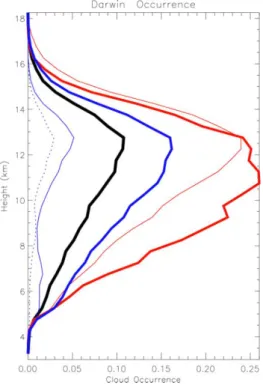
Fig. 1. Vertical profile of the frequency of ice cloud occurrence over Darwin with all regimes included (thick black line), and for the following large-scale atmospheric regimes: Moist Easterly (thick blue line), Easterly (thin solid blue line), Dry Easterly (thin dotted blue line), Active monsoon (thick red line), and Shallow Westerly (thin red line).

The fifth regime, which is found 25 % of the time, exhibits a shallow westerly wind below about 2 km height, with weak easterly winds above that level. The meridional winds are southerly throughout the depth of the troposphere. The mois-ture profile shows a larger dewpoint depression than the Deep Westerly regime. It will be referred to as the “Shallow West-erly” regime.

In addition to the study of the variability of the ice cloud properties as a function of this large-scale atmospheric regime, we will also revisit the description given in PAL09 of the statistical properties of the ice clouds themselves from the four years of observations that have been processed. These results are indeed more robust statistically than those re-ported in PAL09 which was using only data from one wet season (five months) and allow for the upper part of the tro-posphere to be fully characterized in terms of dominant mi-crophysical processes, which was not the case in PAL09.

3.1 Frequency of ice cloud occurrence

The frequency of ice cloud occurrence (which will be re-ferred to as “cloud occurrence” in the following) is defined as the ratio of the number of “cloudy” radar and/or lidar gates to the total number of radar-lidar gates. The most interesting

(6)

31 Figure 1: Vertical profile of the frequency of ice cloud occurrence over Darwin with all regimes included

(thick black line), and for the following large-scale atmospheric regimes: Moist Easterly (thick blue line),

Easterly (thin solid blue line), Dry Easterly (thin dotted blue line), Active monsoon (thick red line), and

Shallow Westerly (thin red line).

Figure 2: Time-height cross-section of the frequency of ice cloud occurrence (in %) over the Darwin site with

all regimes included (a), and for the following large-scale atmospheric regimes: Easterly (b), Dry Easterly (c),

Active Monsoon (d), Shallow Westerly (e), and Moist Easterly (f).

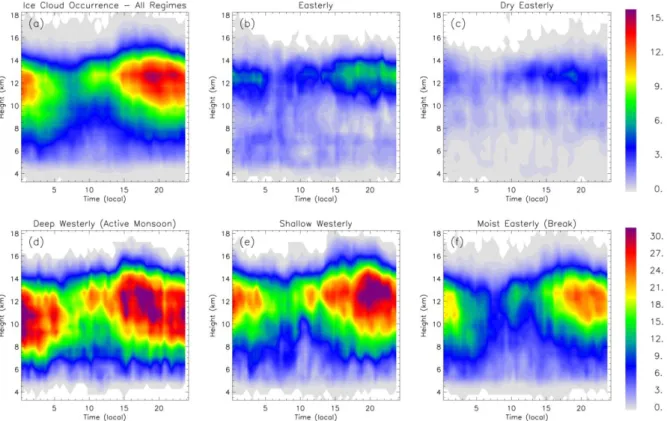
Fig. 2. Time-height cross-section of the frequency of ice cloud occurrence (in %) over the Darwin site with all regimes included (a), and for the following large-scale atmospheric regimes: Easterly (b), Dry Easterly (c), Active Monsoon (d), Shallow Westerly (e), and Moist Easterly (f).

Figure 3: Time series of the vertically-integrated ice cloud occurrence over Darwin with all regimes included (thick black line), and for the following large-scale atmospheric regimes: Moist Easterly (thick blue line),

Easterly (thin solid blue line), Dry Easterly (thin dotted blue line), Active monsoon (thick red line), and Shallow Westerly (thin red line).

Figure 4: Probability Distribution Function (PDF) of cloud top height (a) and geometrical cloud thickness (b) with all regimes included (thick black line), and PDF difference (regime-total) for the following large-scale atmospheric regimes: Moist Easterly (thick blue line), Easterly (thin solid blue line), Dry Easterly (thin dotted

blue line), Active monsoon (thick red line), and Shallow Westerly (thin red line).

Fig. 3. Time series of the vertically-integrated ice cloud occurrence over Darwin with all regimes included (thick black line), and for the following large-scale atmospheric regimes: Moist Easterly (thick blue line), Easterly (thin solid blue line), Dry Easterly (thin dotted blue line), Active monsoon (thick red line), and Shallow Westerly (thin red line).

properties to investigate for this type of quantity are the mean vertical profile (Fig. 1) and the diurnal cycle (Figs. 2 and 3). In order to characterize the amplitude of diurnal

varia-tions of the frequency of ice cloud occurrence, the vertically-integrated frequency of occurrence has been calculated and displayed as times series (Fig. 3). The mean vertical profile obtained when all regimes are considered (thick black line in Fig. 1) shows that the ice cloud occurrence peaks at 12.5– 13 km, reaching a value of 11 %. Figures 2a and 3 show that the diurnal cycle of ice clouds is well marked over Darwin with larger occurrences of ice clouds at night and smallest occurrences in the morning, with a maximum occurrence of 15 % at 13 km between 17:00 and 23:00 Local Time (LT). From There are 2.2 times more ice clouds at 20:00 LT than at 08:00 LT (Fig. 3). also Ice clouds are however also fre-quent during daytime from 8 to 15 km height (Fig. 2a). This daytime signature corresponds to the occurrence of the non-precipitating ice anvils and long-lived cirrus clouds gener-ated by the night-time deep convective activity, which pro-gressively get thinner and with lower cloud tops during their life cycle.

The variability of ice cloud occurrence as a function of the large-scale atmospheric regime (classification of Pope et al., 2009) is very large (Fig. 1). The Easterly and Dry East-erly regimes are characterized by a much smaller ice cloud occurrence throughout the troposphere (5 and 3 % peak val-ues) and a bimodal distribution peaking at 13 km (cirrus) and 6.5 km (altostratus/altocumulus). The three other regimes,

(7)

which occur predominantly during the wet season, are char-acterized by much larger occurrences. The cloud occurrence peaks at the same 12.5 km height as the mean profile for the Shallow Westerly regime (peak value of 23 %) and the Break regime (peak value of 15 %). Cloud occurrence is largest at all heights up to 13 km height during the Active Monsoon regime, but peaks at a lower height (11.5 km). The largest oc-currence of ice cloud at altitudes greater than 13 km is found during the Shallow Westerly Regime (Fig. 1). The lower al-titude of the peak production of ice clouds during the active monsoon is in the result of weaker updrafts in monsoonal convection than during break conditions (PAL09).

The maximum CTHs reached during each regime can be estimated from the envelope of upper-level ice cloud occur-rences in the panels of Fig. 2. The maximum CTHs asso-ciated with the evening convective activity are much larger than those associated with the early morning convection for the Active Monsoon, Shallow Westerly, and Break regimes. This again indicates that convection is more intense and the probability of updrafts overshooting the tropopause largest in the evening convection. During the Break regime, the evening convection in the Darwin area is often associated with squall lines (Keenan and Carbone, 1992), which are well organized and characterized by a large horizontal ex-tent and large updrafts which may explain these highest cloud tops associated with the evening convection.

There are general similarities between the diurnal varia-tions of ice cloud occurrence in each individual large-scale atmospheric regime (Fig. 2), with a maximum in ice cloud occurrence systematically found at night, and a minimum oc-currence around 07:00–10:00 LT. However, the diurnal am-plitude is very different (difference between maximum and minimum frequency of occurrence in Fig. 3). For the Dry Easterly and Easterly regimes, the amplitude of the diur-nal variations is small (0.2 and 0.15, respectively) when compared to the diurnal amplitude of 1.0 obtained when all regimes are grouped together. The Break, Active Monsoon and Shallow Westerly regimes are in contrast characterized by substantially larger diurnal amplitude (1.9, 1.8, and 2.5, respectively).

It is also observed in Fig. 3 (and also in Fig. 2) that the production of ice clouds starts earlier during the Active Mon-soon (around 13:00 LT, with a 33 % maximum occurrence between 15:00 and 19:00 LT) and peaks three hours earlier (17:00 LT) than during the Shallow Westerly and the Break regimes (Fig. 3), corresponding to the earlier triggering of convection during Active Monsoon regime. We also note two layers of slightly enhanced occurrence (also seen on the mean vertical profiles of Fig. 1): cirrus at around 9 km height during the Dry Easterly regime (preferentially in the evening) and altostratus or altocumulus from 5 to 7 km for the easterly regime (preferentially in the morning).

32

Figure 3: Time series of the vertically-integrated ice cloud occurrence over Darwin with all regimes included (thick black line), and for the following large-scale atmospheric regimes: Moist Easterly (thick blue line),

Easterly (thin solid blue line), Dry Easterly (thin dotted blue line), Active monsoon (thick red line), and Shallow Westerly (thin red line).

Figure 4: Probability Distribution Function (PDF) of cloud top height (a) and geometrical cloud thickness (b) with all regimes included (thick black line), and PDF difference (regime-total) for the following large-scale atmospheric regimes: Moist Easterly (thick blue line), Easterly (thin solid blue line), Dry Easterly (thin dotted

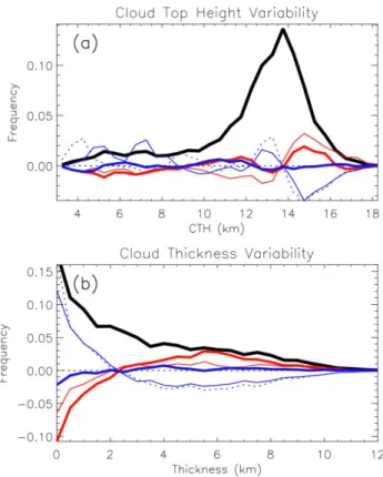
Fig. 4. Probability Distribution Function (PDF) of cloud top height (a) and geometrical cloud thickness (b) with all regimes included (thick black line), and PDF difference (regime-total) for the fol-lowing large-scale atmospheric regimes: Moist Easterly (thick blue line), Easterly (thin solid blue line), Dry Easterly (thin dotted blue line), Active monsoon (thick red line), and Shallow Westerly (thin red line).

3.2 Cloud top height and geometrical thickness

The CTH and thickness statistics are basic but crucial quan-tities for model evaluation purposes, for the evaluation of spaceborne passive remote sensing retrievals of these quanti-ties, and for an accurate estimate of the cloud-radiation feed-backs. The mean ice CTH and thickness PDFs derived from all regimes are given in Fig. 4 (black thick line), as well as the difference between the PDF for each regime and the mean PDF (other lines). The CTH PDF over Darwin (Fig. 4a) is characterized by a bimodal distribution, with a main peak at 14 km height and a secondary peak in the 5–7 km layer. The thickness distribution (Fig. 4b) is dominated by thin clouds, with a roughly exponential decrease in frequency of thicker clouds. The variability of these two macrophysical quanti-ties as a function of the large-scale atmospheric regimes is large and is primarily determined by the wind regime (west-erly or east(west-erly). The west(west-erly regimes tend to generate a larger amount of clouds with tops higher than 13.5 km (up to 16 km for the Active Monsoon regime, up to 18 km for the Shallow Westerly regime, Fig. 4a). Unsurprisingly, this

(8)

33 Figure 5: HPDF of cloud fraction when all regimes are included (a). Percentage differences in frequency with

respect to the HPDF of panel (a) for the following large-scale atmospheric regimes: Active Monsoon (b),

Shallow Westerly (c), Moist Easterly (d), Easterly (e), and Dry Easterly (f).

Figure 6: Mean vertical profiles of the microphysical and radiative properties of ice clouds: (a) ice water

content (in gm

-3

), (b) visible extinction (in km

-1

), (c) effective radius (in



m) and (d) total concentration (in

L

-1

) over Darwin.

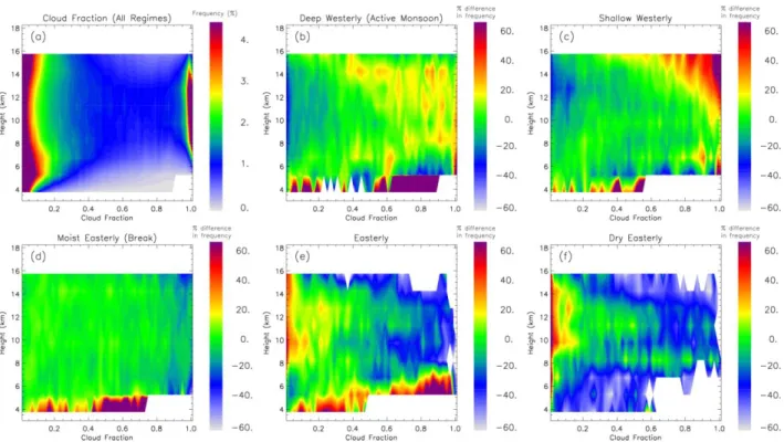
Fig. 5. HPDF of cloud fraction when all regimes are included (a). Percentage differences in frequency with respect to the HPDF of panel (a) for the following large-scale atmospheric regimes: Active Monsoon (b), Shallow Westerly (c), Moist Easterly (d), Easterly (e), and Dry Easterly (f).

increase in frequency of high cloud tops during the Active Monsoon regime is associated with twice as many occur-rences of cloud thickness from 4 to 8 km (Fig. 4b), which reflects the more frequent production of thick anvils by deep convective systems. The Break regime CTH and thickness PDFs are similar to the mean PDFs. The easterly regimes tend to have enhanced frequencies of cloud tops in the 12– 14 km height range, and much smaller frequencies of tops higher than 14 km. This enhancement correspond primarily to clouds of thickness smaller than 2 (thin cirrus), the fre-quencies of which increase by about 50 % during both the Easterly and Dry Easterly regimes. It is noteworthy when comparing the monsoon and break curves of CTH variability that there is a slightly larger occurrence of clouds with tops higher than 16 km during the break period, which is consis-tent with the signature also observed on the upper-level en-velope of the diurnal cycle occurrence of ice clouds which peaks at greater altitudes during the Break periods (Fig. 2). However, the greatest occurrences of highest cloud tops are reached during the Shallow Westerly regime and not during the Break (Fig. 4a), which had not been documented yet to our knowledge. The diurnal cycle plots of Fig. 2e shows that these high cloud tops are reached preferentially from 14:00 to 21:00 LT during the Shallow Westerly regime.

3.3 Cloud fraction

The cloud fraction describes the percentage of the volume of a model grid box filled with clouds. It is one of the two prog-nostic variables to describe an ice cloud in state-of-the-art cloud parameterisations of large-scale models. Cloud frac-tion from cloud radar and lidar observafrac-tions is estimated in the present study exactly as in PAL09 (and also as in Mace et al., 1998; Hogan et al., 2001; Bouniol et al., 2010). The hor-izontal wind field used to define time intervals for the cloud fraction calculations comes from an interpolation of the 6-hourly and 12-6-hourly radiosonde measurements performed over Darwin. For these calculations we have considered three horizontal grid sizes (10, 20, and 40 km) and the 50 verti-cal levels of the Met-Office Unified model, because the next step of this study is to evaluate the representation of clouds in different forecasts using this same model with these three horizontal resolutions over Australia. Results presented in the present paper are however only for the 20 km grid, as the use of the other grid sizes yielded exactly the same conclu-sions. In the present study, only HPDFs of cloud fraction are analysed. Indeed as argued in Bouniol et al. (2010) for mid-latitude clouds, mean vertical profiles of cloud fraction are not a relevant tool for model evaluation, because most of the time and for most heights the cloud fraction distribu-tion is not mono-modal. This appears to be true as well in

(9)

the Tropics. Indeed Fig. 5a does exhibit the same U-shaped type of distribution as at mid-latitudes, with 98 % of the ice clouds characterized either by a cloud fraction smaller than 0.3 or larger than 0.9. When separating the data using the large-scale atmospheric regimes of Pope et al. (2009), several interesting features appear. Firstly, the westerly regimes tend to generate more ice clouds with high cloud fractions (Fig. 5b and c) than when the total sample is considered (Fig. 5a): 20–30 % more clouds during monsoon regime with fraction between 0.3 and 0.95, and up to 40 % more clouds of cloud fraction between 0.95 and 1. In the Shallow Westerly regime the largest effect is above 10 km height, where up to 40–60 % more clouds are characterized by a fraction of 0.8 or higher, while 40 % fewer clouds are with cloud fraction of 0.2 and smaller at these heights. The opposite signature is found in the easterly regimes, characterized by a lower occurrence of ice clouds with high cloud fractions. During the Easterly and Dry Easterly regimes this effect is large, with a 40 to 60 % decrease in occurrence of cloud fractions larger than 0.6–0.7 above 8 km, and a 30–50 % increase in occurrence of cloud fractions smaller than 0.1. This corresponds to a larger production of thin cirrus clouds. As for the frequency of ice cloud occurrence and the macrophysical properties, these large differences definitely have to be well reproduced by cloud parameterizations in order to well simulate the ra-diative effect of clouds.

3.4 Microphysical and radiative properties

As discussed in Sect. 2, the microphysical and radiative prop-erties of ice clouds analysed in this paper were derived using the variational radar-lidar technique of DH08. The main ad-vantage of the DH08 technique is that it allows the radar-only, radar-lidar and lidar-only cloud samples to be included in the statistics. A short summary of the principle of the re-trieval technique and a discussion about the expected errors are given in Protat et al. (2010).

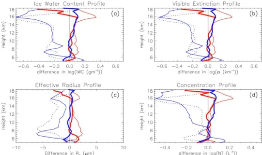
This study provides a good opportunity to update the characterization of the statistical microphysical and radiative properties of tropical ice clouds and their vertical variability using four years of observations at Darwin instead of a sin-gle wet season as was done in PAL09. In particular, the use of many more observations allows a better characterization of the microphysical properties in the upper troposphere. In PAL09 an increase in IWC and extinction above 12 km was observed and was suspected to be an artefact due to the much smaller number of points at these altitudes. The mean verti-cal profiles of the IWC and extinction (Fig. 6a and b) show confirm that this signature is real, but that at heights greater than 15 km (which could not be characterized in PAL09 ow-ing to too few data points), IWC and extinction then decrease rapidly with height. The new results presented in Fig. 6 show that the part of the troposphere where ambient tem-peratures are negative can be split into three distinct layers characterized by different statistically-dominant

microphys-ical processes from cloud top down (that is, for increasing temperatures): layer 1 from 18 km to 15 km, layer 2 from 15 km to 9 km, and layer 3 from 8 km to the melting layer height (around 5 km during the wet season). Statistically speaking layer 1 is characterized by a sharp increase in IWC, extinction and Re, and a relatively constant NTfrom 18 km

down to 15 km height. This suggests that in addition to the expected homogeneous nucleation process at these heights, which would tend to increase IWC, extinction and Re, but

NT as well (which is not the case here), diffusional growth

(also called “deposition”) and ice particle sorting with height by sedimentation in this layer seem to be important micro-physical processes too above 15 km height. Regarding layer 2, IWC is found to slightly increase for decreasing altitudes in the layer, while extinction slightly decreases and total con-centration decreases very rapidly. As discussed in McFar-quhar et al. (2007), the fact that NTdecreases at a much faster

rate than extinction is the signature of aggregation as a dom-inant process because it means that there is a more efficient removal of small ice particles than of large particles. It ap-pears therefore that statistically in this layer aggregation is a dominant process, which is in agreement with the observed predominance of ice aggregates at these temperatures in trop-ical ice anvils (e.g. Heymsfield et al., 2007). However it is also seen that IWC slightly increases, which cannot be the result of aggregation, expected to occur at constant IWC. The observed slight mean increase in IWC with decreasing height in layer 2 probably results from a complex balance between the other microphysical processes which are thought to be potentially important such as riming and diffusional growth, which would both tend to increase IWC without changing

NT. Unfortunately, the observations available here do not

allow further identification of individual microphysical pro-cesses. In layer 3, all the microphysical parameters tend to decrease from 8 km down to the melting layer, which is likely due to the increasing importance of sublimation at the ice cloud bases with respect to aggregation. It is important to note that this result does not mean that sublimation is the dominant mechanism in the first 3 km above cloud base of each individual cloud, because the signatures we discuss here merely reflect the relative importance of microphysical pro-cesses in a statistical sense, combining all types of clouds with all possible cloud heights, bases, and thicknesses. It is also observed in Fig. 6c that the transition from increas-ing effective radii to decreasincreas-ing effective radii for decreasincreas-ing altitudes occurs at a lower height (around 7.5 km) than for IWC and extinction (around 9 km). This result indicates that aggregation in the layer from 9 to 7.5 km is still effective at increasing particle size while sublimation starts removing the small particles. At altitudes lower than 7.5 km it is also ob-served that NT decreases at a rate much larger than above

7.5 km, which indicates that sublimation is increasingly ef-fective at removing small ice particles (and therefore reduc-ing total concentration) in this lower layer.

(10)

33

Figure 5: HPDF of cloud fraction when all regimes are included (a). Percentage differences in frequency with respect to the HPDF of panel (a) for the following large-scale atmospheric regimes: Active Monsoon (b),

Shallow Westerly (c), Moist Easterly (d), Easterly (e), and Dry Easterly (f).

Figure 6: Mean vertical profiles of the microphysical and radiative properties of ice clouds: (a) ice water content (in gm-3_{), (b) visible extinction (in km}-1_{), (c) effective radius (in}__{m) and (d) total concentration (in}

L-1) over Darwin.

Fig. 6. Mean vertical profiles of the microphysical and radiative properties of ice clouds: (a) ice water content (in g m−3), (b) visible extinction (in km−1), (c) effective radius (in µm) and (d) total concentration (in l−1)over Darwin.

Figure 7: PDFs of the microphysical and radiative properties of ice clouds: (a) ice water content (in gm-3), (b) visible extinction (in km-1), (c) effective radius (in m) and (d) total concentration (in L-1) over Darwin with

all regimes included (thick black line), and PDF difference (regime-total) for the following large-scale atmospheric regimes: Moist Easterly (thick blue line), Easterly (thin solid blue line), Dry Easterly (thin dotted

Figure 8: Mean vertical profiles of the difference (regime-total) in microphysical and radiative properties of ice clouds: (a) ice water content (in gm-3), (b) visible extinction (in km-1), (c) effective radius (in m) and (d)

total concentration (in L-1) over Darwin for the following large-scale atmospheric regimes: Moist Easterly (thick blue line), Easterly (thin solid blue line), Dry Easterly (thin dotted blue line), Active monsoon (thick

red line), and Shallow Westerly (thin red line).

Fig. 7. PDFs of the microphysical and radiative properties of ice clouds: (a) ice water content (in g m−3), (b) visible extinction (in km−1), (c) effective radius (in µm) and (d) total concentration (in l−1)over Darwin with all regimes included (thick black line), and PDF difference (regime-total) for the following large-scale atmospheric regimes: Moist Easterly (thick blue line), Easterly (thin solid blue line), Dry Easterly (thin dotted blue line), Active monsoon (thick red line), and Shallow Westerly (thin red line).

The variability of the microphysical and radiative proper-ties as a function of the large-scale atmospheric regime is characterized by the PDF and mean vertical profiles differ-ences (Fig. 7 and Fig. 8, respectively). The first striking fea-ture is that the Easterly and Dry Easterly regimes are

char-acterized by much smaller values of the microphysical pa-rameters over the whole ice part of the troposphere. Dur-ing these regimes ice particle effective radii are smaller at all heights (Fig. 8c) and in much smaller concentrations espe-cially in the upper troposphere (Fig. 8d). Therefore the ice

(11)

clouds during Easterly and Dry Easterly regimes apparently carry much less ice water content (Figs. 7a and 8a) and pro-duce much less visible extinction on average than during the other regimes, especially above 13 km height. The maximum difference in log(IWC) and log(α) is −0.6 at 16 km height, which corresponds to a −0.004 g m−3 difference (or a fac-tor 5) for an average IWC of 0.005 g m−3, and a −0.22 km−1 difference (or a factor 4) for an average α of 0.3 km−1, which are the mean values at 16 km height (see Fig. 6). These large differences are not surprising: a vast majority of ice clouds during these regimes are cirrus clouds, and these cir-rus clouds are not produced by deep convection as in the other regimes but presumably by the instabilities induced by the dynamics of the upper-level jet. From Fig. 7c, it is seen that ice clouds in these regimes are characterized by larger occurrences of particles in the 20–40 µm effective ra-dius range and a reduction in occurrence of particles larger than 50 µm. The mean vertical profiles of difference (Fig. 8c) show that this corresponds to particles being on average 6 mi-crons smaller at 7 km for the Easterly regime and at 8.5 km for the Dry Easterly regime. As was observed for the other cloud properties analysed so far, the Break regime seems to be characterized by microphysical properties similar to those derived from all regimes together. The westerly regimes are generally characterized by larger values for the microphys-ical parameters than the easterly regimes. Both the Active Monsoon and Shallow Westerly regimes produce larger oc-currences of IWC in the range 0.01 to 0.1 g m−3 (Fig. 7a) and of extinction in the range 0.3 to 3 km−1(Fig. 7b). These regimes differ very clearly in terms of effective radius and NT

distributions though. The Active Monsoon regime is char-acterized by larger occurrences of effective radii larger than 40 µm but smaller occurrences of NT larger than 100 l−1,

while the Shallow Westerly regime is characterized by ex-actly the opposite signatures. This translates into larger mean particle sizes mostly in the 6–10 km layer and around 16 km for the Shallow Westerly regime, and much larger total con-centrations in the 15–18 km layer (Fig. 8). The larger oc-currences of larger particle radii seem to occur at all heights during the Active Monsoon regime. When all regimes are considered the largest variability between regimes is found in the 6–10 km layer for effective radius (with a maximum of 8.5 µm at 7 km). This difference is expected to produce relatively large differences in terms of radiative impact, as discussed in Protat et al. (2010).

In conclusion the variability of the different ice cloud properties as a function of the large-scale regimes is large and is expected to produce some differences in radiative im-pact of these ice clouds on average and also preferentially at specific heights. These results highlight the importance of evaluating cloud parameterizations held in large-scale mod-els in light of these regimes. The model should be able to reproduce the observed variability.

4 The variability of ice cloud properties as a function of the ISCCP “cloud” regime

Jakob and Schumacher (2008, referred to as JS08 hereafter) applied a cluster analysis to 6 yr of 3-hourly joint histograms of cloud-top pressure and cloud optical thickness over the Tropical Western Pacific region, following earlier work by Rossow et al. (2005). Using this cluster analysis, six cloud regimes have been defined. Among these six regimes, four regimes correspond to occurrences of ice clouds (70 % of our 4-yr sample), the other two regimes referring to low-level clouds (30 % of our 4-yr sample). Therefore only the four ice cloud regimes are considered in the present study and are de-scribed briefly in what follows. The first ice cloud regime is characterized by large amounts of optically thick clouds with high tops. This signature likely indicates large systems with extensive stratiform cloud coverage, as discussed in JS08, and is referred to as the “Convectively-active Deep cloud (CD)” regime. The CD regime occurs 15 % of the time over the TWP (JS08) and 16 % in our dataset. The second regime also exhibits a large amount of deep cloud but the majority of the cloud occurrence is accounted for by optically thin-ner cirrus clouds. This ice cloud regime is referred to as the “Convectively-active Cirrus (CC)” regime. The frequency of occurrence of the CC regime is larger in our dataset (21 %) than over the TWP region (11 %, see JS08). The third ice cloud regime is a mixture of different cloud types (referred to as the “MIX” regime) in a convectively-active region with no strong generation of large cirrus or anvil clouds. MIX is the most frequent regime in the TWP (33 %, JS08) and in our dataset (29 %). The fourth ice cloud regime occurs in a largely convectively-suppressed environment, and is dom-inated by large amounts of very thin cirrus. This regime will therefore be referred to as the “Suppressed Thin cirrus (STC)” regime. The STC regime is present only 5 % of the time in our dataset (14 % over the TWP, see JS08).

Since the ISCCP cloud regimes are only available up to mid-2007, the variability study described in what follows has been conducted using only the two first years of our dataset.

The variability of ice cloud occurrence as a function of cloud regime is very large (a factor 3 difference in peak ice cloud occurrence among the ISCCP regimes, Fig. 9), as was found with the classification by large-scale atmospheric regime in Sect. 3. The STC cloud regime corresponds fairly well to the sum of the Dry Easterly and Easterly regimes, with a maximum occurrence of 8 % at 12.5 km and a secondary peak in the 5–7 km layer. The three other regimes, which are characterized by a convectively-active environment, are in contrast difficult to link individually to the large-scale at-mospheric regimes in Sect. 3. This is expected, because this type of classification is based on regimes of clouds instead of large-scale atmospheric context. As a result all widespread

(12)

34 Figure 7: PDFs of the microphysical and radiative properties of ice clouds: (a) ice water content (in gm-3_{), (b)}

visible extinction (in km-1), (c) effective radius (in m) and (d) total concentration (in L-1) over Darwin with all regimes included (thick black line), and PDF difference (regime-total) for the following large-scale atmospheric regimes: Moist Easterly (thick blue line), Easterly (thin solid blue line), Dry Easterly (thin dotted

Figure 8: Mean vertical profiles of the difference (regime-total) in microphysical and radiative properties of ice clouds: (a) ice water content (in gm-3), (b) visible extinction (in km-1), (c) effective radius (in m) and (d)

total concentration (in L-1) over Darwin for the following large-scale atmospheric regimes: Moist Easterly (thick blue line), Easterly (thin solid blue line), Dry Easterly (thin dotted blue line), Active monsoon (thick

red line), and Shallow Westerly (thin red line).

Fig. 8. Mean vertical profiles of the difference (regime-total) in microphysical and radiative properties of ice clouds: (a) ice water content (in g m−3), (b) visible extinction (in km−1), (c) effective radius (in µm) and (d) total concentration (in l−1)over Darwin for the following large-scale atmospheric regimes: Moist Easterly (thick blue line), Easterly (thin solid blue line), Dry Easterly (thin dotted blue line), Active monsoon (thick red line), and Shallow Westerly (thin red line).

Figure 9: Same as Fig. 1 but for the ISCCP regimes: CD (blue), STC (green), CC (yellow), and MIX (red).

Figure 10: Same as Fig. 2 but for the ISCCP regimes: CD (b), STC (c), CC (d), and MIX (e).

Fig. 9. Same as Fig. 1 but for the ISCCP regimes: CD (blue), STC (green), CC (yellow), and MIX (red).

stratiform regions or all thick cirrus clouds produced by deep convection (for instance) will be grouped in the same cate-gory instead of being spread out in different ones as in the

large-scale atmospheric regimes in Sect. 3. It is therefore interesting to quantify the variability of the ice cloud prop-erties in each cloud regime as well, because it provides the observational basis for the evaluation of the suitability of cur-rent cloud parameterizations for diffecur-rent well-marked cloud regimes and for the development of cloud-specific parame-terizations. The mean vertical profile of cloud occurrence in the MIX regime, which corresponds to a convective envi-ronment but without a large production of thick anvils and extended cirrus layers, is very similar in shape to the mean profile, but with slightly smaller occurrences than the aver-age at all heights (by 1–2 %). The CC regime is characterized by the largest occurrences, reaching peak values of 26 % at 11–12 km (about twice as much as the average). Finally the CD regime, which includes predominantly the thick anvils produced by deep convection, is characterized by a very dif-ferent vertical profile of cloud occurrence, with larger oc-currences below 11 km height than the average, and also the largest occurrences of ice clouds below 7 km of all regimes, corresponding to the stratiform precipitation and thick non-precipitating anvils produced in deep convective storms. The results for the CC and CD regimes may appear surprising, as the ISCCP data alone indicate a much larger coverage of high-top clouds in the CD regime than in the CC regime (Jakob and Tselioudis, 2003). However, as shown in JS08, the CD regime is primarily characterized by strong precip-itation, both in the convective and stratiform parts of the cloud systems associated with this regime. In our analysis the “convective ice” profiles have been removed (see Sect. 2), so the CD regime as defined in the present analysis is merely

(13)

35

Figure 10: Same as Fig. 2 but for the ISCCP regimes: CD (b), STC (c), CC (d), and MIX (e).

Fig. 10. Same as Fig. 2 but for the ISCCP regimes: CD (b), STC (c), CC (d), and MIX (e).

characterized by thick non-precipitating anvils produced by the deep convective systems. One should therefore treat the forthcoming results of the CD regime with some caution, es-pecially if the results are used to evaluate model clouds. Con-vective ice profiles would have to be removed first from the model profiles using the same method as Sect. 2.

The diurnal variations of ice cloud occurrence are markedly different for each individual regime (Figs. 10 and 11). Figure 10 shows that the STC and CC regimes are char-acterized by the largest diurnal variations (Fig. 10c and e), while the CD and MIX regimes are characterized by rela-tively smaller diurnal variations (Fig. 10b and d). The maxi-mum diurnal amplitude is found in the CC regime (1.8). The much larger frequencies of occurrence found on the mean profiles of Fig. 9 for the CC regimes are observed at all times of day (Fig. 10d, and Fig. 11). This CC regime is also char-acterized by enhanced frequencies of occurrences between 06:00 and 11:00 LT as compared to the other regimes and a reduction of the maximum CTHs from 00:00 to 06:00 LT (Fig. 10b). This corresponds to the progressive thinning and sedimentation of long-lived cirrus clouds generated by the night-time deep convective activity. The MIX regime is char-acterized by diurnal amplitude similar to the average.

There are also marked differences in timing of the max-ima of ice cloud occurrence. In convectively-suppressed conditions (STC regime), ice clouds are produced prefer-entially after 17:00 LT, with a relatively narrow peak oc-currence around 19:00–20:00 LT (Fig. 11). During the CC and MIX regimes, ice cloud occurrence tends to peak later, between 22:00 and 24:00 LT. The diurnal cycle during the CD regime is the most complicated, with multiple peaks (at 05:00, 14:30, and 22:00 LT).

The variability in CTH and thickness obtained when binning our dataset using cloud regimes (Fig. 12) is of similar mag-nitude as when the large-sale atmospheric regimes were used (Fig. 4). The differences in CTH frequencies between cloud regimes is small above 14.5 km and is largest for CTHs rang-ing from 9 to 14.5 km. Durrang-ing the CD regime there is a large increase in CTH frequencies around 10–12 km (by 50 to 100 %) and a drop between 12.5 and 14.5 km, correspond-ing to enhanced thicknesses between 5 and 9 km. The inspec-tion of the diurnal cycle seems to indicate that this signature also corresponds to a less-vigorous early morning convec-tion producing ice clouds at lower heights than in any other regime (from 00:00 to 07:00 LT). The STC and CC cloud regimes are characterized by an enhanced frequency of CTH

(14)

36 Figure 11: Same as Fig. 3 but for the ISCCP regimes: CD (blue), STC (green), CC (yellow), and MIX (red).

Fig. 11. Same as Fig. 3 but for the ISCCP regimes: CD (blue), STC (green), CC (yellow), and MIX (red).

between 11 and 13 km height (by 30 to 50 %). This does not seem to be due to the same reason for both regimes, be-cause the STC regime tends to have larger occurrences of thicknesses smaller than 2 km, while the CC regime has re-duced occurrences of thin clouds and enhanced occurrence of clouds of 5–7 km thickness. This would suggest a produc-tion of more thin cirrus clouds with high tops for the STC regime, and a larger occurrence of shallower convection pro-ducing cirrus at lower heights in the CC regime.

The variability of the cloud fraction distribution in the four cloud regimes is given in Fig. 13. The reference cloud frac-tion distribufrac-tion for this shorter time period is very similar to that given in Fig. 4a and is therefore not shown in Fig. 13. As was also seen when using large-scale atmospheric regimes, there are large differences in cloud fraction distribution be-tween cloud regimes. During the CD and CC regimes, there is substantial increase (>70 %) in ice cloud fractions of 1.0 (very thin line for cloud fraction = 1 in Fig. 13a and c). There is also an increase in the occurrence of intermediate to high cloud fraction in the 6–10 km layer, probably corresponding to larger occurrences of thick cirrus clouds. In contrast, there is a decrease in occurrence of cloud fractions larger than 0.9 for the STC regime (a reduction of about 40 %) and a large increase in cirrus clouds characterized by a very low cloud fraction (60 % more occurrences of cloud fractions <0.05). This result highlights the very different morphology of cirrus produced by deep convection and those produced by upper-level jets in the absence of deep convection.

The mean differences found on the mean vertical profiles (Fig. 15) for the microphysical properties tend to be generally smaller than those found in Fig. 8 when the large-scale atmo-spheric regimes were used. The MIX regime is most similar to the average, with however a tendency to have high-level

Figure 12: Same as Fig. 4 but for the ISCCP regimes: CD (blue), STC (green), CC (yellow), and MIX (red). _{Fig. 12. Same as Fig. 4 but for the ISCCP regimes: CD (blue), STC}

(green), CC (yellow), and MIX (red).

clouds carrying much less ice water content (Fig. 15a) and producing less visible extinction (Fig. 15b), owing to slightly smaller particles (Fig. 15c, Fig. 14c) in smaller concentra-tion (Fig. 15d). This is consistent with the fact that this cloud regime is not expected to include large and persistent cirrus clouds, but rather some optically-thin cirrus (see ISCCP his-tograms in JS08). The CD regime, which includes predomi-nantly stratiform clouds and thick anvils, is characterized by larger occurrences of large particles and smaller occurrences of small particles (Fig. 14c), as also reflected in the enhance-ment of NTof 10–100 l−1and a reduction of the occurrence

of NTlarger than 1000 l−1(Fig. 14d) that is more typical of

high-level cirrus clouds (see mean vertical profile of NT in

Fig. 6d). These characteristics of the CD regime result in larger IWCs in the range 0.01 to 0.1 g m−3_{and larger}

extinc-tions in the range 0.3 to 3 km−1,at all heights (Fig. 15a and b) %. Similar increases in IWC and extinction are also found on the vertical profiles of Fig. 15a and b for the CC regime. However, these signatures are not associated with the same signatures in effective radius and NT as in the CD regime.

In the CC regime, dominated by thick cirrus produced by deep convection, there is only a slight increase in frequency of particles of effective radius larger than 40 µm and smaller occurrences of effective radii ranging from 20 to 40 µm. The frequency of NTlarger than 100 l−1does not drop as in the

CD regime.

The STC regime is characterized by very differ-ent signatures as compared to the convectively-active regimes: smaller particles (Fig. 14c), in larger concentration (Fig. 14d). The impact on the mean vertical profile occurs in two different layers (Fig. 15a and b). In the 15–18 km layer, there is an enhancement of IWC and extinction around 16 km, which can be attributed to the higher frequencies of

(15)

37

Figure 13: Percentage differences in cloud fraction distribution with respect to the HPDF of Fig. 5a for the ISCCP regimes: CD (a), STC (b), CC (c), and MIX (d).

Fig. 13. Percentage differences in cloud fraction distribution with respect to the HPDF of Fig. 5a for the ISCCP regimes: CD (a), STC (b), CC (c), and MIX (d).

occurrence of cirrus clouds around 17:00 UTC in this STC regime (see Fig. 10c). In the 8–10 km layer, IWC, extinc-tion and particle size are also larger than average. A possi-ble explanation for this particular signature is the existence of thick cirrus clouds or altostratus in this regime, produc-ing larger occurrences of large IWC and particle size due to aggregation and diffusional growth in these thick ice clouds. The inspection of the ISCCP histograms in JS08 (their Fig. 1) seems to confirm this point, with some occurrence of clouds of optical depth ranging from 1.3 to 9.4 at these heights for the STC regime.

5 The variability of ice cloud properties as a function of the MJO phase

The Madden-Julian oscillation (MJO; Madden and Julian, 1972) is characterized by eastward migrating regions of strong convection in the Indian and western Pacific Oceans. The intraseasonal variability associated with the MJO is known to modulate the deep convective activity over the Tropics, both near the MJO source region (e.g. Hendon and Liebmann, 1990; Wheeler and McBride, 2005) and remotely through complex teleconnections (e.g. Jones, 2000; Pohl et

al., 2007). It has in particular been shown that it had a large impact on Northern Australian rainfall and circulation (Wheeler et al., 2009), which is the region of interest of our study. As a result it could be expected that the ice cloud pro-duction over the Darwin ARM site by deep convection be also modulated by these large-scale characteristics.

Eight phases of the MJO are defined in Wheeler and Hen-don (2004). The MJO amplitude is defined as significant when greater than 1. The frequency of occurrence of each MJO phase during the four years has been calculated. The frequencies of occurrence of phases 1, 2, 3, 4, 7, and 8 are similar (ranging from 7.5 to 10.5 %), while phases 5 and 6 are found 21 % of the time each. In order to evaluate if there is significant variability of the ice cloud properties as a function of the MJO phase, our data and retrievals have been binned as a function of these MJO phases and the results are presented in a way similar to Sects. 3 and 4.

The variability of the mean vertical profile of the frequency of ice cloud occurrence as a function of MJO phase (Fig. 16) is relatively smaller than the variability induced by binning the dataset into large-scale atmospheric regimes or ISCCP

(16)

37

Figure 13: Percentage differences in cloud fraction distribution with respect to the HPDF of Fig. 5a for the ISCCP regimes: CD (a), STC (b), CC (c), and MIX (d).

Fig. 14. Same as Fig. 7 but for the ISCCP regimes: CD (blue), STC (green), CC (yellow), and MIX (red).

cloud regimes. All vertical profiles but for MJO phases 1 and 8 peak at the same height of 12.5 km. There is neverthe-less a relatively large difference in peak frequencies for three groups of MJO phases. Occurrences during MJO phases 1, 2, and 8 are characterized by the smallest frequencies (around 7 %). Occurrences during MJO phases 3, 4 and 7 are similar to those of the mean vertical profile, with a peak value around 11 %. Finally, largest occurrences of ice clouds are found during phase 5 (15 % peak) and phase 6 (20 % peak). Going back to the study of Wheeler et al. (2009) about the modula-tion of weekly rainfall probabilities by the MJO phase, they show that conditional probabilities of receiving accumulated rainfall in the climatological upper tercile shifts from being less than 20 % in phases 1, 2, and 8 to greater than 60 % in phases 5 and 6 over the Darwin area during austral summer. This variability of rainfall probability therefore appears to be fully consistent with enhanced occurrences of tropical ice clouds in phases 5 and 6, and reduced occurrences for phases 1, 2, and 8. Even the “neutral” phases in terms of likeli-hood of rainfall do correspond to “neutral” phases in terms of ice cloud production. This result shows indirectly again the previously-discussed major role played by deep convec-tion in the producconvec-tion of ice clouds in the upper troposphere, and therefore indirectly the modulation of the production of ice clouds by the phase of the MJO.

The variability in diurnal variations between periods char-acterized by different MJO phases (Fig. 17) is smaller than that identified using cloud regimes and large-scale atmo-spheric regimes, except for MJO phases 3, 5, and 6. The large diurnal amplitude during MJO phase 3 is due to the combi-nation of very small integrated frequencies of occurrences between 07:00 and 13:00 LT and large ones after 17:00 LT (Fig. 18). During MJO phase 5 diurnal amplitudes are only slightly larger than average (1.1 as compared to 1.0, Fig. 18),

which is due to a secondary maximum in occurrence of ice clouds from 08:00 to 13:00 LT (Fig. 17f, Fig. 18) where most MJO phases are characterized by a minimum in occurrence. The diurnal cycle during MJO phase 5 resembles that of the CD cloud regime, which probably indicates that clouds pro-duced during this MJO phase 5 are predominantly optically-thick clouds with high tops in a convectively-active environ-ment (the definition of the CD cloud regime). This is also consistent with Fig. 17f. During MJO phase 6, the diurnal amplitude is large (2.0) and the timing is different, with a production of ice clouds by deep convection earlier than for other MJO phases (maximum at 16:00–17:00 LT, instead of 20:00 LT, see Fig. 17g and Fig. 18).

The vertical distribution of cloud occurrence displayed in Fig. 17 also appears to be quite different between MJO phases. During MJO phases 1, 2, 7 and 8, the largest fre-quencies of occurrences are concentrated in the upper lev-els, as was observed during the Easterly and Dry Easterly regimes (Fig. 2b and c) and during the STC cloud regime (Fig. 10c). In contrast the thickest clouds are produced dur-ing MJO phases 3, 5 and 6. This is consistent with larger vertically-integrated frequencies of ice cloud occurrence in Fig. 18.

The variability in CTH obtained when binning our dataset using MJO phases (Fig. 19) is of similar magnitude as when the large-sale atmospheric regimes (Fig. 4) and the ISCCP cloud regimes (Fig. 12) are used. The variability in thickness among the periods characterized by different MJO phases is in contrast smaller than when the other criteria are used. The MJO phases 1, 2, 7, and 8 (which are those during which less ice clouds are found in Fig. 16) are all characterized

(17)

38

Figure 16: Same as Fig. 1 but for the MJO Phases : left panel for Phases 1 to 4, right panel for Phases 5 to 8. Colour code is given in the Figure.

Fig. 15. Same as Fig. 8 but for the ISCCP regimes: CD (blue), STC (green), CC (yellow), and MIX (red).

Figure 16: Same as Fig. 1 but for the MJO Phases : left panel for Phases 1 to 4, right panel for Phases 5 to 8. Colour code is given in the Figure.

Fig. 16. Same as Fig. 1 but for the MJO Phases: left panel for Phases 1 to 4, right panel for Phases 5 to 8. Colour code is given in the Figure.

by smaller occurrences of CTH larger than 13.5 and larger occurrences of clouds thinner than 1–2 km. Phases 5 and 6 (and to some extent phases 3 and 4 too) are characterized by a larger occurrences of cloud tops higher than 13.5 km. For phase 3 this is due to an increase in the intensity of deep con-vection producing higher (Fig. 17d) and thicker (see increase in 6–9 km cloud thickness frequency) ice clouds from 15:00 to 22:00 LT. For phases 5 and 6 it does not really correspond to a large increase in cloud thickness (Fig. 19d), so it is pre-sumably primarily due to the larger frequency of occurrence of high cloud tops seen between 15:00 and 22:00 LT on the diurnal cycle plots (Fig. 17f, g).

The differences in cloud fraction distributions as a function of the MJO phases are not as obvious as for the large-scale atmospheric regimes and ISCCP cloud regimes. Therefore it has been decided not to show this figure but to summa-rize briefly the salient features. There are essentially two patterns of difference with respect to the average cloud frac-tion distribufrac-tions. The first one is a larger reducfrac-tion of high cloud fractions (by 40 to 60 %) and increase of cloud frac-tions lower than 0.2 for MJO phases 2, 7, and 8 for heights greater than 10 km. The second signature is an increase of the frequency of occurrence of cloud fractions larger than 0.8 by about 20–30 % for MJO phase 5 above 10 km height. In or-der to evaluate if a model is able to reproduce the variability in cloud fraction distributions it seems more appropriate to use the large-scale atmospheric or cloud regimes rather than the MJO phases.

The PDF differences (Fig. 20) show that the IWC and extinc-tion distribuextinc-tions are shifted towards smaller values for the phases associated with smaller ice cloud occurrences (phases 1, 2, 4, 7 and 8). For these five phases it is also seen that the occurrence of effective radii larger than about 40–50 µm is reduced (Fig. 20e, f). As shown in Fig. 21, these reductions in IWC, extinction, and effective radius, are occurring at dif-ferent altitudes for these difdif-ferent phases: during phases 1 and 2, the maximum reduction is around 8 km height; ing phase 4 it occurs between 10 and 14 km height; dur-ing phases 7 and 8 it results in large reductions in the up-per troposphere, with a maximum reduction at 16 km height, except for the effective radius reduction for phase 7 which