TRANSPORTATION INTERFACE by
CHRYSSOSTOMOS CHRYSSOSTOMIDIS B.Sc., University of Durham
(1965)
S.M., Massachusetts Institute of Technology (1967)
Nav. Arch., Massachusetts Institute of Technology (1968)
SUBMITTED IN PARTIAL FULFILLMENT OF THE REQUIREMENTS FOR THE
DEGREE OF DOCTOR OF PHILOSOPHY at the MASSACHUSETTS INSTITUTE OF TECHNOLOGY February, 1970 Signature of Author Certified b Accepted by
Department of Nival Architecture and Marine Engineering, January 8 , 1970
y
Thesis Supervisor
Chairman, Dep rtmental Committee oh Graduate Students
Archives
by
CHRYSSOSTOMOS CHRYSSOSTOMIDIS
Submitted to the Department of Naval Architecture and Marine Engineering on January 8, 1970, in partial fulfillment of the requirements for the degree of Doctor of Philosophy.
ABSTRACT
In this study, two basic tasks have been considered. The first of these was the development of the mathemati-cal model simulating a cargo transportation interface in which the cargo is to be transported from a ship moored at some dis-tance from the shore to point A on a beach where no port facil-ities are available. The transferring of cargo from the ship to the shore is accomplished by means of transfer vehicles, such as amphibious craft. The cargo transfer from the ship to the transfer vehicles is accomplished by ship-based unloading gear, such as ship-based cranes. The cargo transfer from the transfer vehicles at the shore is accomplished by beach-based unloading gear, such as fork lifts.
The second of these was the selection of the solution method that would permit the analysis of such a mathematical model. Importance was attached to the condition that the sol-ution method should enable the user to gain an insight into the unloading procedure and thence to correctly derive the optimum use strategies in the ship-to-shore transfer analysis. The method chosen was that of computer digital simulation be-cause it not only provides the user with the necessary in-sight, but also allows the user to solve the problem at hand without the need for the introduction of drastic simplifica-tions into the mathematical model, as would certainly be re-quired by any of the known optimization techniques. As a further means of enhancing the usefulness of our methodology, the concept of antithetic variance was introduced into our solution procedure. (Antithetic variance is the means by which the user may exercise the underlying [stochastic]
math-ematical model the minimum number of times in order to esti-mate the necessary results with a prespecified degree of con-fidence.)
Because digital simulation is employed as the solution method in almost all congestion problems, it follows that antithetic variance may also be used profitably in models other than the one in this study. Guidelines for the user have therefore been included, wherein the expected usefulness of the concept of antithetic variance (as developed here) in its application to congestion problems in generalis indicated. Thesis Supervisor: Ernst G. Frankel
The research reported in this study was carried
out under the sponsorship of the Office of Naval Research under M.I.T. DSR No. 70562. The author is grateful to the Office of Naval Research for their interest in this subject and for their financial support.
The author also wishes to thank Professors E. G. Frankel, J. W. Devanney III, J. M. Sussman, and P. Mandel of M.I.T. for their continuous encouragement and con-structive ideas at all phases of this study. Finally, the author is indebted to his wife, Margie, for editing and proofreading the final draft, to Mrs. V. Liddell for her excellent typing of the final draft, and to Miss L. Carella and Miss B. Leblanc for helping out with the typing when the deadline was drawing close.
All computations were performed at the Computation
Table of Contents ABSTRACT ... ACKNOWLEDGMENTS ... LIST OF TABLES ... LIST OF FIGURES ... 1. INTRODUCTION .... ... ... 2. SOLUTION PROCESS ... . 3. PROBLEM DEFINITION ...
4. FORMULATION OF THE MATHEMATICAL MODEL ... 5. SOLUTION METHOD .... ...
A. Event Definition ... B. Scheduling Mechanism Definition ... C. Computer Program Description ... D. General Flow Chart ... E. Concept of Antithetic Variance... 6. PROBLEM SOLUTION ... 7. EVALUATION OF RESULTS, CONCLUSIONS, AND
FUTURE RECOMMENDATIONS ... BIBLIOGRAPHY ... ... APPENDIX A - Additional Information Pertaining
the Solution Method... APPENDIX B - Input Data Listing... APPENDIX C - Computer Program Listing ...
BIOGRAPHICAL NOTE ... Page 2 3 5 6 7 10 20 61 100 100 102 105 112 115 168 192 198 201 215 224 307
Table No.
3-1 Processes Describing Breakdown
Considerations ... 6-1 Experimental Data for the Digital
Simulation of a Transportation Interface
Test Cases ... 6-2 Mother Ship's Closure Time ... 6-3 Beach Unloading Facilities'
Closure Time ... 37
170 171
172
6-4 Transfer Vehicle Closure Time ... 173 A-6 Input Data for the Experiment
Leading to Figs. 5-3 and 5-4 ... 214 Page
Block Diagram of Solution Processes ... General Model Construction ... 5-la General F 5-1 lQ-lS Sys 5-2 5-3 " it " " " " General Input Da it I i "f "I i "I " "I " "I "I "I " "I " "I "I "I "I ", " "I " "I "I "I " "I " D t Page 11 .... .... .... 21 low Chart ... 112 tem Mean Customer Waiting Time (n vs al & a 2) . 137 " (r vs p) ... 138
"t " " " for p=0. 90
(1I Vs a. & af) 140
Mean of Mean Customer Waiting Time
vs. Variance ... 141 Mean Time that the Server Remained Idle
(11 vs a2 a?..) ... 150
Mean Time that the Server Remained Idle
for p=0.90 (-n vs oY & a2..) ... 151 Mean Time to Serve 200 Customers
(n vs a2 & 2)... 159
Mean Time to Serve 200 Customers
for p=0.90 (n vs a12 & a) ... 160
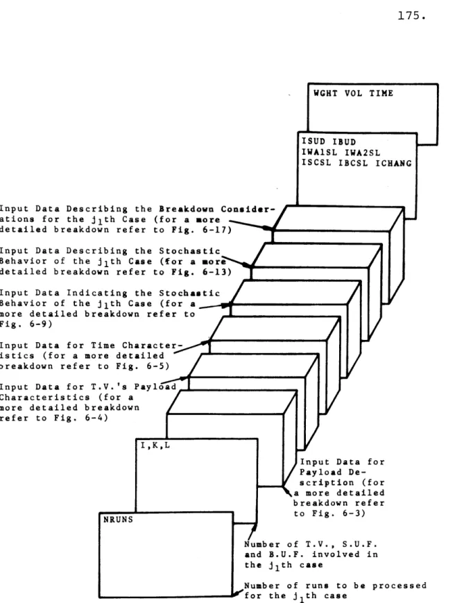
ata Setup ... 174 a Setup for the jjth Case ... 175
" t " "Payload Description ... .176 " " " T.V.'s Payload Charateristics 177 " t " "Time Characteristics ... 178 " f
" "S.U.F's Time Characteristics. 179
" " B.U.F.'s " " . 180 "f " " T.V.'s " " . 181
" t "I Indication of the Stochastic
Behavior of the J1 th Case... 182
5-4 5-5 5-6 5-7 5-8 6-1 6-2 6-3 6-4 6-5 6-6 6-7 6-8 6-9 6-10 6-11 6-12 6-13 6-14 6-15 6-16 6-17 of the Stochastic the S.U.F...183 of the Stochastic the B.U.F...184 of the Stochastic the T.V...185 of the Stochastic the j1 th Case... 186 of the Stochastic the S.U.F... 187 of the Stochastic the B.U.F...188 of the Stochastic the T.V...189 " " "Description of the T.V.'s Breakdown Characteristics...190 6-18 Input Data Setup for STATIC...191 7-1 Weight W)and Volume (V)Utility of Transfer Vehicles...196
No. 2-1
3-1
" " " Indication
Behavior of
"I "I " Indication
Behavior of Indication Behavior of "I " "Description Behavior of "I " "Description Behavior of Description Behavior of Description Behavior of
The basic task of the problem posed is that of develop-ing the methodology that will permit the overall analysis of a cargo offloading procedure. In the offloading procedure under investigation, the cargo is to be unloaded from a ship, henceforth referred to as the mother ship, which is at some distance, say x miles, from the shore. The Mother Ship is to be stationary during the entire unloading operation. The final and only destination of the cargo is to be a point A on the beach. There are to be no port facilities on the shore or beach unloading areas.
The cargo involved in this study is to be contained in
i) Containers or pallets of arbitrary size, weight and capacity that are not capable of any self-induced motion, or
ii) Vehicles of arbitrary size, weight and capacity that are capable of self-induced rolling motion only. It should be noted that in this case the vehicle itself may be the cargo.
The actual transferring from the Mother Ship to the beach is to be accomplished by means of amphibious craft, whose number and characteristics have been prespecified. These are henceforth referred to as the transfer vehicles, such as LARCs, GEMs, etc. The loading into the transfer
independent from the loading mode, the unloading from the transfer vehicles on the beach is to be in one of the two modes: sequential or simultaneous.
In order to accomplish the cargo transfer from the Mother Ship to the transfer vehicles, the Mother Ship is to be pro-vided with all the necessary unloading facilities, for example ship-borne crane(s), ramp(s), etc. However, the transfer
vehicles are not to be provided with any special unloading facilities, because some means, such as a fork lift, is to be made available on the beach to carry out the cargo unloading.
Finally, the prespecified number of transfer vehicles and beach unloading gear is to be made available at point A, and their transportation and arrival is to be independent of that of the Mother Ship, and from each other.
With the above description, the cargo offloading procedure under investigation has been fully defined. In order to complete the description of the problem posed, it remains to define the analysis objectives, which can be
stated as follows: The resulting technique is to be designed to first provide a common measure of success for a number of prespecified use strategies for given ship-based loading facilities, transfer vehicles and beach-based unloading
facilities distributions, for a given x and environment state, and for given breakdown considerations. The common measure
of success is to depend on time and/or the number of
transfer vehicles malfunctioning. Thus the final analysis objective is to determine the best strategy (with respect to
the measure of success mentioned above) among those examined or, if the findings of the previous calculations suggest it, to continue the analysis with new strategies until the
desired one is found. It should be noted that in selecting the measure of success mentioned above the author was limited
by the requirements of the sponsor.
With the above, the problem description has been com-pleted. The solution process is to be outlined in the sub-sequent Sections and Appendices. We start our discussion with a general outline of the solution process.
The solution process in this study is best illustrated by the block diagram shown in Fig. 2-1. A brief discussion of each step involved in the solution process is given below.
Problem Definition. This involved the following: i) Identification of the variables of the problem. ii) Establishment of the relations among the
variables.
iii) Identification of the dependent and independent variables of the problem consistent with i) and
ii).
iv) Establishment of the range of variation of all problem parameters.
v) Selection of the figure of merit. vi) Choice of Use Strategies.
By definition, the variables of a problem are those parameters necessary to fully describe a given system to the
degree of accuracy and extent desired. The process of
variable identification for a new problem, such as ours, is a major and a very difficult task. In order to simplify our
task of identifying our variables, it was found advantageous to first identify the subsystems involved in our study and then find the variables necessary to fully describe each sub-system to the degree of accuracy and extent desired. The subsystems involved in our study were found to be:
Problem Definition Formulation of Mathematical Model Selection of Solution Method Problem Solution Evaluation of Results
BLOCK DIAGRAM OF SOLUTION PROCESS Fig. 2-1
12. 1. The mother ship.
2. The payload.
3. The ship-based unloading facilities, S.U.F.
4. The shore-based unloading facilities, B.U.F.
5. The transfer vehicles, T.V.
The variable identification is deferred until the next Section where the Problem Definition will be discussed in de-tail. It is of importance to note in conjunction with the discussion of the variable identification that although it was recognized that the environment state as described by
1. Wind speed,
2. Sea state,
3. Current,
4. Tide,
5. Obstacles,
6. Beach configuration, and 7. Shore configuration
influences our offloading operation, it was decided to de-scribe their effect by externally adjusting the magnitude of the appropriate parameters. For this reason, it is not neces-sary to identify any variables that describe the environment state. However, when assigning the magnitude of the
parameters that are affected by the environment state, the user must assign the appropriate values by taking the environ-ment state into consideration.
The establishment of the relations, if any, among the problem variables is a necessity as they form a part of the mathematical model. The reason for this is that because the mathematical model is, by definition, the replica of our
sys-tem in the form of mathematical equations, any such relations must be part of it in order to permit it to be a true replica of the original. The establishment of any such relations is deferred until the next Section where the Problem Definition will be discussed in detail.
As was stated at the beginning of this section, the problem variables were so selected that when the appropriate values were assigned to them, they could serve to define a given offloading system uniquely to the degree of accuracy and extent desired. This, however, should not be taken to imply that if we assign arbitrary but logical values to these var-iables we will always be able to generate an offloading system because of the possible interrelations among the variables, which do not permit independent selection of values for all
the interrelated variables. This fact makes it necessary to identify those variables whose values can be assigned arbitrar-ily and those whose value cannot. This is because our solu-tion method involves the evaluasolu-tion of different offloading systems which are generated by prespecifying the values of their variables. This is best done by classifying the var-iables into dependent and independent ones. The independent variables are those variables which must be prescribed to
completely describe our system as desired. The dependent variables are the ones remaining in our original list of variables after the independent ones have been removed. The identification of the dependent and independent variables is deferred until the next Section where the Problem Definition will be discussed in detail.
Ideally speaking, we would like to impose no restric-tions on the range of variation of our problem parameters, other than the ones implied by the physics of our problem, as this will tend to decrease the universality of our methodology. However, there are practical considerations, common to this type of problem, which make it necessary that we impose limits on the range of variation of our problem parameters. The most common of these considerations (requiring us to compromise by imposing limits on the range of variation of our problem
parameters) is that it is impossible to construct the math-ematical model valid over the entire range of variation of the problem parameters. In the few times that it is possible to
construct such a model, it again becomes necessary to restrict the range of variation to simplify the model and make it a useful engineering tool. Therefore, the above indicates the need for the introduction of restrictions as unavoidable. These restrictions, of course, ought to be introduced with great care. Care should be taken because we do not wish to reduce the universality of our methodology unnecessarily, as
we wish to utilize it to solve most, if not all, of the problems that we are likely to encounter, but at the same time we wish to obtain this solution with relative ease and consistent but adequate precision. The introduction of these restrictions is deferred until the next section, when the Problem Definition will be discussed in detail.
As was already mentioned in the Introduction, the figure of merit (the measure of success) is the weighted combination of time and the number of transfer vehicles malfunctioning. The time component of the figure of merit involves the calcu-lation of mean time elapsed since the start of the mission to
1. prepare the mother ship for departure after all
the payload has been transferred into the transfer vehicles, and all transfer vehicles have cleared the mother ship,
2. complete the payload transfer from the mother ship
to point A on the beach,
3. return all transfer vehicles to their bases, and
4. return all beach-based unloading facilities to their bases.
The latter component of the figure of merit involves the calculation of the percentage of transfer vehicles that did not complete their mission because of breakdown. The
factors determining the likelihood of breakdown for each transfer vehicle are:
1. Reliability of the transfer vehicle's components.
2. Hazard vulnerability.
3. Control stability.
4. Operational limitations.
The establishment of the exact nature of the figure of merit is deferred until the next Section where the Problem Defini-tion will be discussed in detail.
Finally, the set of use strategies to be incorporated in the mathematical model of this study were developed. Although it is anticipated that for all cases likely to be encountered in practice, the best strategies may be found among those incorporated into our model, the algorithm is to be made suf-ficiently flexible to allow the introduction of more use
strategies for the investigation of cases not predicted here. The description of the use strategies to be incorporated into our mathematical model is deferred until the fourth section where the mathematical model of our study will be developed.
Formulation of the Mathematical Model.
As was stated earlier, the mathematical model is, by
definition, the replica of our system, to the degree of accur-acy and extent desired, in the form of mathematical equations. Because of the nature of our problem, the mathematical model is stochastic in nature. In setting up the mathematical model care was taken to keep it as simple as possible to permit easy analysis, and yet to construct it so that it exhibits all the
phenomena under consideration, as required. The
actual construction of the mathematical model is deferred until the fourth section.
Selection of Solution Method.
From the Problem Definition one may easily observe that the easiest way to achieve the desired goal, namely, to find the best use strategy, is to treat the use strategy as a prob-lem variable, and then solve the probprob-lem under investigation as an optimization problem. The resulting optimization prob-lem is a mixed integer one, or simply an integer probprob-lem if the waiting times of the transfer vehicles and unloading fa-cilities are approximated by integers. However, it was soon discovered that in order to solve the problem as an optimiza-tion one, drastic simplificaoptimiza-tions had to be made to the math-ematical model to allow us to efficiently implement the solu-tion in present-day computers. The reason for this is that the state description of our system was large. The drastic simplifications necessary made our methodology a very inef-ficient engineering tool. Last, but not least, if the use strategy obtained by solving the problem as an optimization one was very complicated, it probably would have been very difficult to implement in practice (because the system might be operating under external pressure). For this reason it would be very easy to violate a complicated optimum use
cannot be estimated in any way, which is a very
un-desirable situation as it defeats the purpose of this analysis. For the reasons given above it was decided to develop a methodology that will yield the desired solution, not neces-sarily as directly as it would have been provided by the op-timization theory, but one which
1. could be implemented without requiring major
simplifications in the mathematical model, and 2. could test logical and likely "optimal" use
strategies which have a very high probability of being implemented in practice.
The method that satisfied all the above requirements was the digital simulation method, which was utilized in this study to obtain the desired solution. By this method the desired solution was obtained by testing different use strat-egies that satisfied the second requirement given above. To develop these use strategies, one is guided by logic, es-pecially in developing the first use strategy to be tested, and by the insight gained from the previous tries when this is available. The discussion of the actual details of the methodology used in this study is deferred until the fifth section.
Problem Solution
This involves the preparation of the input required by the computer program. Special care must be taken when pre-paring the input of the parameters, whose magnitude is affected by environment state and breakdown considerations. Further discussion on this topic is deferred until later.
Evaluation of Results
With reference to Fig. 2-1, special care was taken that the only iteration required in the Solution Process is the preparation of new input data for the examination of a new use strategy, if the Evaluation of Results suggests it. It is anticipated that there will never be any need for the al-teration of the first three steps of Fig. 2-1, as care was taken to make the methodology developed here general, in order to handle all cases likely to be encountered in prac-tice. However, if a case arises where a change must be intro-duced in these three steps, the user must read very carefully the next three sections so that he may correctly alter the present method to suit nis needs. Further discussion on this
topic is deferred until later.
The above completes the introduction in the Solution Process. In the next section a detailed presentation of the Problem Definition will be given.
3. Problem Definition
In this section a detailed discussion of each step in-volved in the Problem Definition is given.
i) Identification of the Problem Variables
In view of the fact that the smaller the number of variables in a problem the more economical, and in many
in-stances the more efficient, the solution process becomes, an attempt was made to keep the number of variables of this
problem to a minimum. To do so it was necessary to introduce certain assumptions. However, special care was taken so that the nature and number of these assumptions was such as not to diminish the generality of our methodology. These assumptions will be enumerated in the fourth topic of this section, when
the range of variation of the problem parameters is discussed.
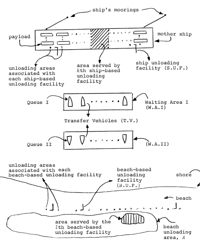
As was mentioned earlier, in order to simplify our task of identifying our problem variables, the subsystems involved in our study were identified. These are shown
diagrammatically in Fig. 3-1. For presentation purposes, the variables that are utilized to define each subsystem and at the same time appear in the computer input will be listed first, while the remaining variables necessary to complete each subsystem's description will be given later.
payload unloading areas associated with each ship-based unloading facility ship's moorings mother ship
area served by ship unloading kth ship-based facility (S.U.F.) unloading facility Queue I W (1 aiting Area I W.A. I) Transfer Vehicles (T.V.) Queue II (W.A.II) unloading areas
associated with each
beach-based unloading facility
beach-based
unloading shore
facility (3.U.F.)
beach
area served by the
Zth beach-based beach
unloading facility unloading
area, A
MOTHER SHIP DESCRIPTION
The variables* selected to describe the Mother Ship's performance are:
TAM giving the number of units of time after the start of the mission that the Mother Ship is expected to arrive in the theater of operations [-999<TAM<9999 (treated as a floating point number)].
T1 giving the number of units of time required to com-plete the mooring operations of the Mother Ship after it arrived in the theater of operations [0.<T1<9999
(treated as a floating point number)].
T2 giving the number of units of time required to free the Mother Ship from its moorings and make ready to travel after all S.U.F. are secured to position and all T.V. have cleared the Mother Ship [0.<T2<9999
(treated as a floating point number)].
IDMA** indicating the nature of the process concerning the arrival of the Mother Ship.
ID1** indicating the nature of the process concerning the
mooring operation of the Mother Ship.
ID2** indicating the nature of the process concerning the
operation of freeing the Mother Ship from its moorings.
*The magnitude of all the variables selected to describe the Mother Ship's performance except the magnitude of
INMS, IN1, IN2 and TIME is affected by environmental state.
**IDMA, ID1, ID2 = 1 if the process is deterministic.
= 2 if the process is stochastic, drawn from U(0,1) distribution.
= 3,4... 9999 if the process is stochastic, drawn from distributions to be devel-oped by the user, if so desired.
INMS giving the seed of the U(0,1) distribution, which serves to predict the stochastic behavior of the Mother Ship's arrival process, if IDMA = 2***
[1<INMS<10 9-1].
AMINM giving the minimum value of the range of variation of
TAM, if IDMA = 2***[-999.99999 < AMINM < 9999.99999]. AMAXM giving the maximum value of the range of variation of
TAM, if IDMA = 2***[-999.99999 < AMAXM < 9999.99999]. IN1 giving the seed of the U(0,1) distribution, which
serves to predict the stochastic behavior of the Mother Ship's mooring operation, if ID1 = 2* [1<IN1<109-1].
AMIN1 giving the minimum value of the range of variation of T1 if ID1 = 2h[O.<AMIN1<9999.99999]
AMAX1 giving the maximum value of the range of variation of T1 if ID1 = 2*[0.<AMAX1<9999.99999].
IN2 giving the seed of the U(0,1) distribution, which
serves to predict the stochastic behavior of the opera-tion of freeing the Mother Ship from its moorings,
if ID2 = 2**[1<ID2<10 9-1].
AMIN2 giving the minimum value of the range of variation of
T2 if ID2 = 2**[O.<AMIN2<9999.99999].
AMAX2 giving the maximum value of the range of variation of
T2 if ID2 = 2**[O.<AMAX2<9999.99999].
TIME giving the units of time utilized in this study
[0 < TIME < 12 alpha numeric characters].
*If ID1=1 IN1, AMIN1 and AMAX1 are not problem variables.
**If ID2=1 IN2, AMIN2 and AMAX2 are not problem variables.
PAYLOAD DESCRIPTION
The variables selected to describe the payload are:
Nk giving the number of payload units to be unloaded by each
of the k (k = 1,2.. .K) S.U.F. K
1
< Nk
<
1000 and
N
<
1000}
K WCn giving the weight of each of the n n = 1,2... 1 Nk
k=1
payload units plus that of their lashings [0.<WCn <99.99]. K
VC giving the volume of each of the n n = 12 ... N
n kn-12.
k=1 payload units together with that of their lashings*
[0.<VC <9999 (treated as a floating point number)].
WGHT giving the units of weight utilized in this study
[0<WGHT<12 alpha numeric characters].
VOL giving the units of volume utilized in this study
[0<VOL<12 alpha numeric characters].
*If all the T.V. employed in this study do not permit vertical stowing of the payload, VC can be utilized to give the volume
n
per unit height plus the surface area required by their
lash-K
ings rather than the volume of each of the n (n=1, 2... k1Nk payload units and that of their lashings, as this is a quan-tity much easier to estimate.
The variables* selected to describe the S.U.F.'s per-formance are:
K giving the number of S.U.F.** involved in this case 1 < K < 20]
ISUD*** indicating the nature of the unloading mode at the Mother Ship.
ISCSL**** indicating which of the S.U.F. use strategies is to
be used.
TS 1,k giving the time required for the kth (k = 1,2.. .K)
S.U.F. to be made ready to start the unloading
oper-ation and reach the kth ship unloading area after the Mother Ship is properly moored [0. < TSC1,k
< 9999 (treated as a floating point number)].
* The magnitude of all the variables selected to describe the S.U.F. 's performance except the magnitude of INSCj k
(j 2 = 1,2 ... 5,7,8,9; k = 1,2 ... K) is affected
by the environment state.
** Each S.U.F. is identified by a distinct number, k, such
that 1 < k < K.
* ISUD = 1 if the unloading mode at the Mother Ship is to be in parallel. ISUD = 2 if the unloading mode at the Mother Ship is to be sequential.
* If ISCSL = 1, S.U.F. use strategy SLSCA is used to select the appropriate S.U.F. when necessary.
- 2, S.U.F. use strategy SLSCB is used to select the appropriate S.U.F. when necessary.
= 3, S.U.F. use strategy SLSCC is used to select the appropriate S.U.F. when necessary.
- 4,5.. .9, additional S.U.F. use strategies to
be developed by the user, if desired, for selecting the appropriate S.U.F. when necessary.
TSC2,k giving the time required for the kth (k = 1,2...K)
S.U.F. to travel to any of theNkpayload units from the kth ship unloading area [0. < TSC2,k < 9999 (treated
as a floating point number)].
TSC3,k giving the time required to release any of the Nk
(k = 1,2...K) payload units after the kth S.U.F.
has reached the payload unit in question [0. < TSC3,k
< 9999 (treated as a floating point number)].
TSC4,k giving the time required to secure any of the Nk
(k = 1,2.. .K) payload units on the kth S.U.F. after the payload unit in question has been released
[0. < TSC4,k < 9999 (treated as a floating point
number)].
TSC5,k giving the time required to transport any of the Nk
(k = 1,2.. .K) payload units to the kth ship unloading area after the payload unit in question has been se-cured on the S.U.F. [0. < TSC6,k < 9999 (treated as a
floating point number)].
TSC7,k giving the time required to unload and then free any of the Nk (k = 1,2...K) payload units from the kth
S.U.F. and to then make the kth S.U.F. ready to
travel again. This operation is performed only if (a) the appropriate T.V. is properly secured in the kth ship unloading area and has completed its refuel-ing (if refuelrefuel-ing was necessary), (b) the previous payload unit unloaded by the S.U.F. in question is fully secured in the T.V. in question (this require-ment is void if the payload unit in question is the first payload unit to be unloaded in any of the T.V.'s trips), and (c) the T.V.'s remaining capacity can accept the payload unit in question. If any of the above is not satisfied, the kth S.U.F. must wait
TSC?,k until all three requirements are satisfied
(cont'd.) [0. < TSC < 9999 (treated as a floating point
number)].
TSC8,k giving the time required for the kth (k = 1,2.. .K)
S.U.F. to travel back to its original position
from the kth ship unloading area after the last of the Nk payload units has been transferred onto the appropriate T.V. [0. < TSC8,k < 9999 (treated as a
floating point number)].
TSC 9 k giving the time required for the kth (k = 1,2...K) S.U.F. to be secured to its original position.
IDSC * indicating the nature of each of the
j
2 = 1,2...2 ...5,7,8,9) processes described above for each of
the k (k = 1,2.. .K) S.U.F. INSC j 2 , k AMINSC. AMAXSC.7 J2 k *IDSC 2' k
giving the seed of the U(0,1) distribution, which serves to predict the stochastic behavior of each of the j 2 (2 = 1,2...5,7,8,9) processes described above
for each k (k = 1,2...K), if IDSC. = 2**
[1 < INSCJ2,k < 101
giving the minimum value of the range of variation of TSCJ2 k (, = 1,2... 5,7,8,9; k = 1,2...K), if
IDSC. k2** [0. < AMINSC < 9999.99999].
giving the maximum value of the range of variation of TSC. (j2 = 1,2.. .5,7,8,9; k = 71,2... K), if
(2,k
IDSC. = 2** [0. < AMAXSC < 9999.99999]. = 1 if the process is deterministic.
= 2 if the process is stochastic, drawn from U(0,1) distribution.
= 3,4.. .9999 if the process isstochastic, drawn from distributions to be developed by the user, if so desired.
**If IDSC =1 INSC 2, AMINSC 2 k and AMAXSC are not
B. U.F. DESCRIPTION
The variables* selected to describe the B.U.F.'s per-formance are:
L giving the number of B.U.F.** involved in this case [1 < L < 20].
IBUD*** indicating the nature of the unloading mode at the beach.
IBCSL**** indicating which of the B.U.F. use strategies is to
be used.
TBC 13 giving the number of units of time after the start of the mission that the Zth (k = 1,2...L) B.U.F. is
expected to depart from its base [-999 < TBC <
1,9.-9999 (treated as a floating point number)].
*The magnitude of all the variables selected to describe the B.U.F.'s performance except the magnitude of
INBC. (j4 = 1,2.. .4,6,7... 10; Z = 1,2.. .L)
is affected by environment state.
**Each B.U.F. is identified by a distinct number, k, such that 1 < k < L.
***IBUD = 1 if the unloading mode at the beach is to be in parallel.
= 2 if the unloading mode at the beach is to be se-quential.
****If IBCSL = 1, B.U.F. use strategy SLBCA is used to select the appropriate B.U.F. when necessary.
= 2, B.U.F. use strategy SLBCB is used to select the appropriate B.U.F. when necessary.
= 3,4.. .9, additional B.U.F. use strategies to be
developed by the user if so desired, for selecting the appropriate B.U.F. when necessary.
TBC2 . giving the time required for the kth (k = 1,2.. .L)
B.U.F. to reach point A on the beach from its base
[0. < TBC2 . < 9999 (treated as a floating point
number)].
TBC giving the time required for the kth (Z = 1,2...L) B.U.F. to be made ready to start the unloading
opera-tion after the kth B.U.F. has arrived at point A on
the beach [0. < TBC 3 , < 9999 (treated as a floating point number)].
TBC43k giving the time required for the kth (k = 1,2.. .L)
B.U.F. to travel to the kth beach unloading area from
point A on the beach after the 9th B.U.F. has been made ready to travel [0. < TBC4 < 9999 (treated as
a floating point number)].
TBC6,1 giving the time required to release any of the pay-load units utilizing the kth (k = 1,2... L) B.U.F. This operation is performed only if the appropriate T.V. is beached and ready to commence the unloading operation and the kth B.U.F. has reached the kth beach unloading area. If that is not the case, the
releasing of the payload unit must wait until the two requirements given above are satisfied [0. < TBC6,Z
< 9999 (treated as a floating point number)].
TBC73Z giving the time required to secure any of the payload units on the 9th (k = 1,2.. .L) B.U.F. after the
pay-load unit has been released [0. < TBC7 < 9999
(treated as a floating point number)].
TBC8,Z giving the time required after the payload unit in question has been secured on the Zth (Z = 1,2.. .L)
.U.F. to (a) transport any of the payload units from
the 9th beach unloading area to point A on the beach
TBC8,k payload unit from the kth B.U.F. and (c) make the
(cont'd.) Pth B.U.F. ready to travel again [0. < TBC < 8, 2
-9999 (treated as a floating point number)]. TBC giving the time required to prepare the Zth
(z = 1,2...L) B.U.F. for departure after it has
terminated its mission [0. < TBC < 9999 (treated
as a floating point number)].
TBC giving the time required for the kth (Z = 1,2.. .L)
B.U.F. to reach its base after it has been made
ready for departure [0. < TBC 10, < 9999 (treated as a floating point number)].
IDBC. 4 * indicating the nature of each of the j4 (j4=
1,2,3,4,6,7 ... 10) processes described above for each of the Z (k = 1,2...L) B.U.F.
INBC j1 giving the seed of the U(0,1) distribution which serves to predict the stochastic behavior of each of
the j4 (j4 = 1,2,3,4,6,7...10) processes described above for each k (k = 1,2...L), if IDBC. =2**
J34
[1 < ITNBC . < 109 1]
AMINBC . giving the minimum value of the range of variation
of TBC (j4 = 1,2,3,4,6,7.. .10; = 1,2.. .L), if
IDBC. = 2** [-999.99999 < AMINBC < 9999.99999;
0. < AMINBC. < 9999.99999,
j3
= 2,3,4,6,?... 10].AMAXBC. giving the maximum value of the range of variation
of TBC. (j4 = 1,2,3,4,6,7.. .10; = 1,2.. .L), if IDBC. = 2** [-999.99999 < AMAXBC < 9999.99999;
0. < AMINBC. < 9999.99999, j3 = 2,3,4,6,7...10].
*IDBC. = 1 if the process is deterministic.
04, = 2 if the process is stochastic, drawn from
U(0,1) distribution.
= 3,4...9999 if the process is stochastic, drawn from distributions to be developed by the user, if so desired.
**If IDBC I -=1, then INBC - , AMINBC* and AMA XBC
The variables* selected to describe the T.V.'s perform-ance are:
giving the number of T.V.** involved in this case
( 1 < I < 20).
IWA1SL*** indicating which of the T.V. use strategies is to be used in W.A.I.
IWA2SL**** indicating which of the T.V. use strategies is to be used in W.A.II.
* The magnitude of the variables IWA1SL, IWA2SL, ICHANG, AMAXTV 7 i (i = 1,2.. .1), TTV (j =1 2,4... 7,9,10,11,13, 15,16,1), IDTVi (j =1,2.0,1.13516, 17)
AMINTV -- and' AMA TV- is affected by the environment
state. The magnitude oi the variables WT1MAX, WT2MAX,
IDBRTV - (j9=1,2.. .8) BRKTV. - is affected by the
envir-onment 9'state and breakdown 0S'©considerations.
** Each T.V. is identified by a distinct number, i, such that
1 < i < I.
If IWA1SL = 1, T.V. use strategy ASLTVA
-2, T.V. use strategy ASLTVB
- 3, T.V. use strategy ASLTVC -4, T.V. use strategy ASLTVD
= 55,6,7,8, T.V. use strategy ASLTVE
is used to select the appropriate T.V. from W.A.I when necessary.
= 9, additional T.V. use strategy to be devel-oped by the user, if so desired, for
selecting the appropriate T.V. from W.A.I when necessary.
* If IWA2SL = 1, T.V. use strategy BSLTVA
= 2, T.V. use strategy BSLTVB = 3, T.V. use strategy BSLTVC
= 4, T.V. use strategy BSLTVD
is used to select the appropriate T.V. from W.A.II when necessary.
= 5,6.. .9, additional T.V. use strategies to be developed by the user, if so desired, for selecting the appropriate T.V. from W.A.II when necessary.
T.V. use strategy indicator
AMAXTV
6 giving the weight of payload together with that of
the associated lashings that the ith (i = 1,2.. .I) T.V. can carry in any of its trips [0. < AMAXTV i
6, 9 <9999 (treated as a floating point number)].
* If ICHANG = 1, the T.V. use strategies specified by the user at the outset of the investigation of a case will be used throughout the simulation of the case under investigation.
= 2, the T.V. use strategies specified by the user at the outset of the investigation of a case will be changed automatically with the
fol-lowing rules.
i) If IWA13L = 1, the instant the weight
payload of a T.V. is violated, IWA1SL
and IWA2SL assume the value 2.
ii) If IWA1SL = 3, the instant the weight
payload of a T.V. is violated, IWA1SL
and IWA2SL assume the value 4.
iii) If IWA1SL = 2 the instant the volume payload of a T.V. is violated, IWA1SL and IWA2SL assume the value 1, and
iv) If IWAlSL = 4 the instant the volume
payload of a T.V. is violated, IWA1SL
and IWA2SL assume the value 3.
32.
AMAXTV giving the volume of payload together with that of
7
the associated lashings that the ith (i = 1,2.. .I) T.V. can carry in any of its trips. Note that the definition of units of AMAXTV . must be'the same as
K
that of VC (n = 1,2.. k 1N k [0 < AMAXTV . < 99999
n k-7 ,i
-(treated as a floating point number)].
TTV _ giving the number of units of time after the start of the mission that the ith (i = 1,2... I) T.V. is expected to depart from its base [-999 < TTV < 9999 (treated as a floating point number)
TTV23 giving the time required for the ith (i = 1,2.. .1)
T.V. to reach W.A.I from its base [0. < TTV <
9999 (treated as a floating point number)]
TTV 4 . giving the time required for the ith (i = 1,2.. .I) T.V. to reach and hook up to any of the ship unload-ing areas from W.A.I and prepare the ith T.V. for the loading operation. Note that the ith T.V. can leave W.A.I only when there is a ship unloading area free to receive it. [0. < TTV4 . < 9999 (treated as
a floating point number)].
TTV . giving the time required for the ith (i = 1,2...1)
T.V. to refuel, when necessary, after it has hooked up at any of the ship unloading areas [0. < TTV5 i 9999 (treated as a floating point number)].
TTV6,i giving the time expected for the ith (i=1,2...I) T.V. will operate at other than zero speed, during a complete cycle. [0. < TTVi < 9999 (treated as a floating point number)].
TTV 7 . giving the time expected that the ith (i = 1,2... 1) T.V. will operate at, other than zero speed, without refueling. [0. < TTV 7 i < 9999 (treated as a
TTV giving the time required for any payload unit to be secured on the ith (i = 1,2...1) T.V. after it has
been unloaded into the ith T.V. and freed from the appropriate S.U.F., and after the S.U.F. in question has been made ready to travel again [0. < TTV 9 . < 9999 (treated as a floating point number)].
TTV71 . giving the time required for the ith (i = 1,2... I) T.V. to unhook and be made ready to travel after the last payload unit unloaded into the ith T.V. has been properly secured. [0. < TTV 10, < 9999 (treated as a floating point number)].
TTV 1 1 giving the time required for the ith (i = 1,2.. .1)
T.V. to reach W.A.II from any of the ship unloading areas [0. < TTV 1 i < 9999 (treated as a floating point number)].
TTV 1 3 giving the time required for the ith (i = 1,2.. .1) T.V. to reach any of the beach unloading areas from W.A.II and then beach and be made ready for the un-loading operation. Note that the ith T.V. can leave W.A.II only when there is a beach unloading area free to receive it [0. < TTV 13i < 9999 (treated as a
float-ing point number)].
TTV1 5,i giving the time required for the ith (i = 1,2...I)
T.V. to be made ready to travel again after the last payload unit carried on any of its trips has been se-cured to the appropriate B.U.F. [0. < TTV 1 5 < 9999
(treated as a floating point number)].
TTV1 6,i giving the time required for the ith (i = 1,2...1) T.V. to reach W.A.I from any of the beach unloading areas after it has been made ready to travel [0. < TTV 16i 9999 (treated as a floating point number)].
TTV17,
IDTV. 7*
INTV
AMINTV J
AMAXTV.
giving the time required for the ith (i = 1,2.. .I) T.V. to reach its base from any of the beach un-loading areas after it has completed its mission
[0. < TTV < 9999 (treated as a floating point
number)].
indicating the nature of each of the j7 (1,2...5,9,
10...13,15,16,17) processes described above** for each of the i (i = 1,2...1) T.V.
giving the seed of the U(0,1) distribution which serves to predict the stochastic behavior of each of the j 7 (j 7 = 1,2.. .5,9,10.. .13,15,16,17)
pro-cesses described above for each i (i = 1,2...I), if
IDTV. =2*** [1 < ITNTV. . < 109 -]
giving the minimum value of the range of variation
of TTV. (j7 = 1,2.. .5,9,10...13,15,16,17; i = 077 1,2.. .1), if IDTV. .=2***[-999.99999 < AMINTV 1 < 0 7 ,' I-9999.99999; 0. < AMINTV. . < 9999.99999, j8 = 2, 3... 5,9,10 ... 13,15,16,17].
giving the maximum value of the range of variation
of TTV J (4 = 1,2.. .5,9,10.. .13,15,16,17; i =
1,2.. .1), if IDTV. . = 2*** [-999.99999 < AMAXTV 1
< 9999.99999; 0. < AMAXTV.1 .< 9999.99999 , =
2 38,1 1- l08
2,3.. .5,9,10... 13,15,16,1?].
*IDTV. .=1 if the process is deterministic.
07"&=2 if the process is stochastic, drawn from U(0,1) distribution.
=3,4... 9999 if the process is stochastic, drawn from distributions to be developed by the user, if so desired.
**Processes 3 and 12 are associated with the waiting of a T.V. in W.A.I and W.A.II respectively.
6 and 7 are always deterministic.
***If IDTV. .=1,then INTV. ., AMINTV. . and AMAXTV.
WT1MAX giving the maximum time that any of the I T.V. is expected to wait in W.A.I at any time during the mission [0. < WT1MAX < 9999999.99].
WT2MAX giving the maximum time that any of the I T.V. is expected to wait in W.A.II at any time during the mission [0. < WT2MAX < 9999999.99].
IDBRTV. * indicating the presence or absence of breakdown
considerations for each of the
j
9(j
9 = 1,2...8)processes (see Table 3-1) for the ith (i= 1,2...I) T.V. and, in the event that breakdown
considera-tions are present, their nature.
giving the seed of the U(0,1) distribution which serves to predict the stochastic behavior of each of the j, (iJ = 1,2.. .8) processes described
above for each i (i = 1,2...1), if IDBRTV. .=2**
[1 < INBRTV. .< 109 -1].9
giving the probability that a breakdown will occur during the j th (j = 1,3,4,6,7,8) process for each i (i = 1,2.. .1), and the probability that a breakdown will occur if the ith T.V. waited WT1MAX or more units of time in W.A.I during the 2nd
process*** and the probability that a breakdown will occur if the ith T.V. waited WT2MAX or more
units of time in W.A.II during the 5th process***,
if IDBRTV. . =2** [0. < BRKTV. . < 1.0000].
*IDBRTV. . = 1 if there are no breakdown considerations.
- 2 if there are breakdown considerations which
are drawn from a U(0,1) distribution.
= 3,4...99 if there are breakdown considerations which are drawn from distributions to be
devel-oped by the user, if so desired.
** If IDBRTVj ,i=1., thenINBRTVj 3 and BRKTVj9 are not
prob-lem variables.
* If the T.V. waited less the probability is scaled down linearly.
INBRTV. .
39 = 1 Describes the breakdown considerations of each T.V. regarding its trip to W.A.I from its base. The breakdown considerations of this process are a function of the T.V. involved.
= 2 Describes the breakdown considerations of each T.V. regarding
its waiting in W.A.I. The breakdown considerations of this process are a function of the T.V. involved and the waiting time.
= 3 Describes the breakdown considerations of each T.V. regarding its trip to any of the ship unloading areas from W.A.I. The breakdown considerations of this process are a function of the T.V. involved.
= 4 Describes the breakdown considerations of each T.V. regarding its trip to W.A.II from any of the ship unloading areas. The breakdown considerations of this process are a function of the T.V. involved.
= 5 Describes the breakdown considerations of each T.V. regarding its waiting in W.A.II. The breakdown considerations of this process
are a function of the T.V. involved and the waiting time.
= 6 Describes the breakdown considerations of each T.V. regarding its trip to any of the beach unloading areas from W.A.II. The breakdown considerations of this process are a function of the T.V. involved.
= 7 Describes the breakdown considerations of each T.V. regarding its trip to W.A.I from any of the beach unloading areas. The breakdown
considerations of this process are a function of the T.V. involved.
= 8 Describes the breakdown considerations of each T.V. regarding its
trip to its base from any of the beach unloading areas. The breakdown considerations of this process are a function of the T.V. involved.
Table 3-1
With the above, the list of the variables that are
utilized to define the five subsystems involved in our study and at the same time appear as input in our computer program is complete. There exist two additional inputs to the com-puter program which serve to control the program's performance and which for the sake of completeness we include here. These are:
NCASES giving the number of cases to be processed in
each program execution [1 < NCASES < 99], and NRUNS giving the number of runs to be processed for
the j1th (j1 = 1,2...NCASES) case [1 < NRUN < 500].
We continue now by listing the remaining variables neces-sary to complete each subsystem's description.
MOTHER SHIP DESCRIPTION
The additional variables selected to complete the descrip-tion of the Mother Ship's performance are:
TAMP, T1P, T2P* giving the time fluctuation associated with
TAM, T1 and T2 respectively.
TTM giving the total time taken by the Mother Ship to com-plete its operation. This includes the time taken to
free the Mother Ship from its mooring and to make it ready for travel again after all S.U.F. are secured in position and all T.V. have cleared the Mother Ship.
If IDMA and/or ID1 and/or ID2 equal 1, then TAMP and/or T1P
and/or T2P equal zero respectively. If that is not the case,
TAMP, T1P and T2P are determined by drawing from the
appro-priate distribution, as dictated by the magnitude of IDMA,
39.
PAYLOAD DESCRIPTION
The variables given above suffice to describe the pay-load characteristics to the degree of accuracy and extent desired, and so no additional variables are needed.
S. U. F. DESCRIPTION
The additional variables selected to complete the
descrip-tion of the S.U.F. 's performance are:
TSC, k giving the time that the kth (k = 1,2.. .K) S.U.F.
has to wait in the kth ship unloading area before it can unload the payload unit that it is trans-porting. The kth S.U.F. has to wait until the appropriate T.V. is properly secured in the kth
ship unloading area or until the previously un-loaded payload unit is properly secured in the T.V. in question. (This process is always deterministic.) TSCP j, k* giving the time fluctuation associated with TSC
2, k
(22 = 1,2... 5,?,8,9; k = 1,2.. .X ).
AMAXSC6,k giving the total time taken by the kth (k= 1,2...K)
S.U.F. to complete its mission. This includes the
time taken to secure the S.U.F. in its original position.
*If IDSC . equals 1, then TSCP . k equals zero. If that is
not the case, TSCP.2,k is determined by drawing from the appropriate distribution, as dictated by the magnitude of IDSC.
40.
B. U. F. DESCRIPTION
The additional variables selected to complete the description of the B.U.F.'s performance are:
TBC 5, k
TBCP. *
AMAXBC 5, 9
giving the time that the kth (k = 1,2...L) B.U.F.
has to wait in any of the beach unloading areas before it can release the appropriate payload unit. The kth B.U.F. has to wait in a beach un-loading area until the appropriate T.V. is properly beached and has been made ready for the unloading operation. (This process is always deterministic.)
giving the time fluctuation associated with TBC. £ (j4 = 1,2,3,4,6,7...10; k = 1,2...L).
giving the total time taken by the kth (Z = 1, 2... L)
B.U.F. to complete its mission. This includes the
time taken for the kth B.U.F. to reach its base.
*If IDBC . equals 1, then TBCP . equals zero. If that is not the case, TBCP . is determined by drawing from the
appropriate distribution, as dictated by the magnitude of