HAL Id: hal-00808611
https://hal.archives-ouvertes.fr/hal-00808611
Submitted on 9 Apr 2013
3D Reconstruction from SECCHI-EUVI Images Using
an Optical-Flow Algorithm: Method Description and
Observation of an Erupting Filament
Samuel Gissot, Jean-François Hochedez, Pierre Chainais, Jean-Pierre Antoine
To cite this version:
Samuel Gissot, Jean-François Hochedez, Pierre Chainais, Jean-Pierre Antoine. 3D Reconstruction
from SECCHI-EUVI Images Using an Optical-Flow Algorithm: Method Description and Observation
of an Erupting Filament. Solar Physics, Springer Verlag, 2008, 252 (2), pp.397-408. �hal-00808611�
DOI: 10.1007/•••••-•••-•••-••••-•
3D Reconstruction from SECCHI-EUVI Images
Using an Optical-Flow Algorithm: Method
Description and Observation of an Erupting Filament
S.F. Gissot1,2, J.-F. Hochedez1, P. Chainais3,
J.-P. Antoine2
Received ; accepted c
° Springer ••••
Abstract SECCHI-EUVI telescopes provide the first EUV images enabling a
3D reconstruction of solar coronal structures. We present a stereoscopic recon-struction method based on the Velociraptor algorithm, a multiscale optical-flow method that estimates displacement maps in sequences of EUV images. Follow-ing earlier calibration on sequences of SoHO-EIT data, we apply the algorithm to retrieve depth information from the two STEREO viewpoints using the SECCHI-EUVI telescope. We first establish a simple reconstruction formula that gives the radial distance to the centre of the Sun of a point identified both in EUVI-A and EUVI-B from the separation angle and the displacement map. We select pairs of images taken in the 30.4 nm passband of EUVI-A and EUVI-B, and apply a rigid transform from the EUVI-B image in order to set both images in the same frame of reference. The optical flow computation provides displacement maps from which we reconstruct a dense map of depths using the stereoscopic reconstruction formula. Finally we discuss the estimation of the height of an erupting filament.
Keywords: Chromosphere: Active, Prominences: Dynamics, Formation and
Evolution, Technique: 3D reconstruction, Stereoscopy, Optical Flow
1. Introduction
The complexity of magnetic structures of the solar corona is well observed in EUV observations of the Sun. In EUV images of the solar atmosphere, loops and filaments appear as compact structures that are well observed at the limb and
1 Solar Influences Data analysis Centre, Royal Observatory
of Belgium, Avenue Circulaire 3, B-1180 Brussels, Belgium (e-mail: [email protected], [email protected])
2 Unit´e de Physique Th´eorique et de Physique
Math´ematique - FYMA, Universit´e catholique de Louvain, Chemin du Cyclotron 2, B-1348 Louvain-la-Neuve, Belgium
3 LIMOS, Universit´e Blaise Pascal Clermont II, 63173
on the disc when compared to the surrounding fuzzy corona. In the latter case, there remains an ambiguity on the height of the features. In order to solve the third dimension, two points of view are necessary to perform a stereoscopic re-construction. The height of EUV bright points has been estimated and analyzed in Brajˇsa et al. (2004) using the method proposed by Rosa et al. (1998). Similar work has been achieved on filament height estimation (Vrˇsnak et al., 1999). Since the launch of the STEREO mission (Kaiser et al., 2007), it is possible to resolve the 3D ambiguity by using the observation of the two viewpoints STEREO-A and STEREO-B. First loop reconstructions have been published in Feng et al. (2007) using a loop extraction (Inhester et al., 2007). A method for stereoscopic reconstruction and epipolar geometry has been proposed (Inhester, 2006). We present a method for retrieving the depth information from a pair of STEREO-SECCHI-EUVI images observed on-board the two spacecrafts of the STEREO mission using simple geometrical facts and a novel algorithm,
Velociraptor (Gissot et al., 2003; Gissot and Hochedez, 2007), to estimate the subpixel displacement. The Velociraptor algorithm is a multiscale optical flow algorithm derived from a local gradient-based technique able to estimate displacement and brightness variation maps in solar extreme-ultraviolet images as recorded by the Extreme ultraviolet Imaging Telescope (EIT) on board the Solar and Heliospheric Observatory (SoHO) and by the Transition Region and Coronal Explorer (TRACE). Here the displacement maps to estimate are shifts along the epipolar line caused by the separation of the two STEREO viewpoints, and no brightness variation is supposed: this method is here applied to estimate the height of an erupting filament.
2. 3D Reconstruction Method
In this section we present the method for retrieving the altitude information from a pair of STEREO images. In the following we will refer to the image observed in EUVI on-board STEREO spacecraft STEREO-A and STEREO-B as EUVI-A and EUVI-B, respectively. We introduce two heliocentric-Cartesian coordinate systems SAand SB with notation (x,y,z), that both have their origin
at the Sun centre O, with y normal to the STEREO mission plane (STEREO-A,STEREO-B,O) and z pointing to solar disc centre of either EUVI-A (system
SA), or EUVI-B (system SB). In the following, the index A (resp. B) refers to
the coordinate system SA (resp. SB). The objective is to measure the radius
R = OP of a point P of coordinates (XA,YA,ZA) in SA and (XB,YB,ZB) in
SB. After the pre-registration step, the point P observed in EUVI-A is seen in
EUVI-B as P0, i.e. as P rotated by an angle of ∆λ. 2.1. Pre-registration
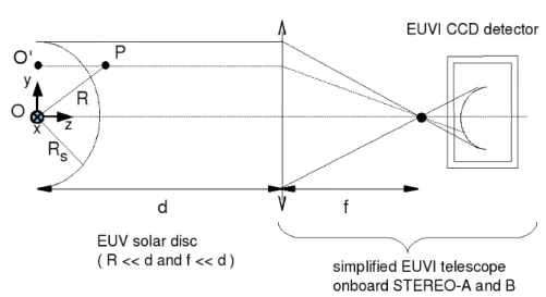
Since the Sun may be assumed to be at an infinite distance of STEREO-A and of STEREO-B, Figure 3 shows that in both instruments the solar disc as traced by its limb is the orthogonal projection of the solar sphere of centre O and photospheric radius Rs as observed in EUVI-A. In the following, the separation
Figure 1. STEREO mission plane (STEREO-A, STEREO-B, O) and ecliptic north axis.
The SA and SB coordinate systems have their origin at the Sun centre O and their y-axis
perpendicular to (STEREO-A, STEREO-B, O) and z pointing either to STEREO-A (SA) or
STEREO-B (SB).
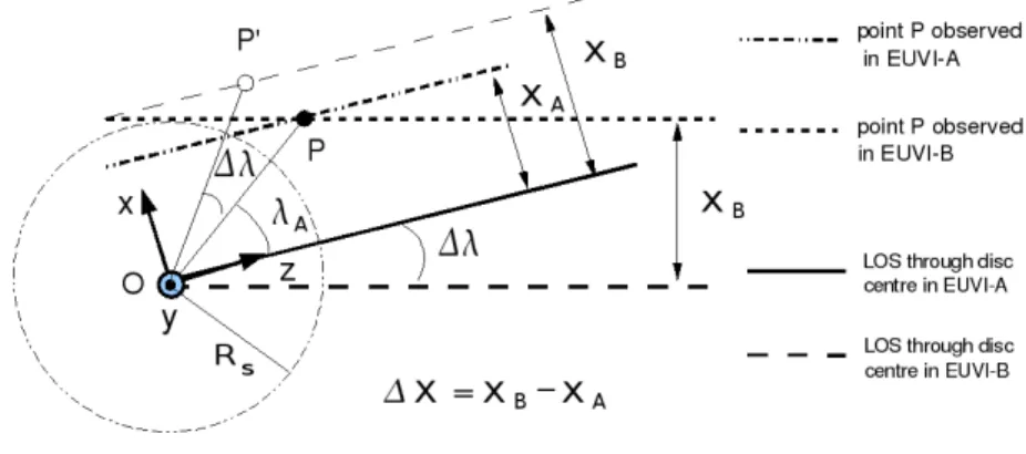
Figure 2. Apparent displacement ∆X of P after the pre-registration step applied to EUVI-B
so that it can be matched with EUVI-A. The point P appears as P0in EUVI-B where P0is the point P rotated by ∆λ.
angle between spacecrafts is denoted by ∆λ, λA is the angle of P to Oy, R is
the distance of P to the Sun centre, (XA,YA,ZA) (resp. (XB,YB,ZB)) are the
coordinates of P in SA(resp. SB) (see Figure 4). Figure 2 shows that observing
P on the solar sphere from two different viewpoints (spacecrafts STEREO-A
and STEREO-B) is equivalent to observing, from one unique viewpoint, the point P in EUVI-A rotated to a virtual point P0 by an angle ∆λ. Indeed the displacement
Figure 3. The projection model of the sun in the EUVI detectors of the STEREO spacecrafts
STEREO-A and STEREO-B.
is equal to the apparent displacement of P moving to P0after a rotation of angle ∆λ and centre O (see Figure 4). Observed in EUVI-B, the point P is equal to
P0 of coordinates (XB,YB,ZB) in SA.
This equivalence requires three conditions: the pointing to the heliospheric centre
O must be known with precision, the radius of the solar limb must be the same
in EUVI-A and EUVI-B (or equivalently, the distance from STEREO-A and STEREO-B to O must be known with precision), and the axis of the rotation, or the normal to the STEREO mission plane containing A, STEREO-B and O (see Figure 1) must be known as well. If we impose that this axis be vertical in both image planes, the last requirement ensures that the epipolar lines are horizontal if we neglect the projective geometry effects, so that YA = YB.
The pre-registration step consists in transforming EUVI-B using translation, rotation, and dilation, in order to set EUVI-B in the same reference frame as EUVI-A so that both image centres are pointing to the Sun centre, they both have the same apparent photospheric radius Rs, and their vertical axis is aligned
with the epipolar north. After applying the pre-registration procedure that reads the information contained in the FITS headers, EUVI-A and B now have:
• the line-of-sight (LOS) of the image centres passing through the Sun centre O (after a translation),
• the vertical axis perpendicular to the plane containing
(STEREO-A, STEREO-B, O), see Figure 1 (after a rotation),
• the same limb radius equal to the photospheric radius Rs from EUVI-A
(after a dilation). This dilation is achieved using the distance to the Sun of both spacecrafts.
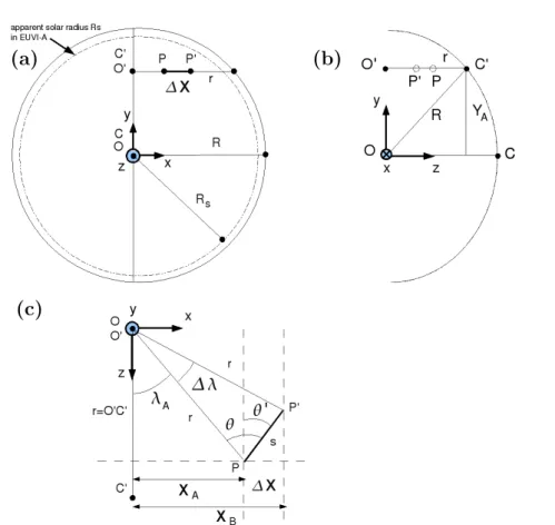
(a)
(b)
(c)
Figure 4. Representation of the angles λA, ∆λ, θ, the radii r and R, and the distance s. Rs
is the photospheric radius as observed in EUVI-A. After the pre-registration step, both images EUVI-A and -B are in the same frame of reference. Figure (a): front view from STEREO-A (EUVI-A) image. Figure (b): left view. Figure (c): top view.
2.2. 3D Reconstruction Formula
In Figure 4 the point P becomes P0after a rotation of the sphere by an angle ∆λ. The line OC shows the LOS passing through the apparent disc centre (Figure 2) and pointing to the heliospheric centre O, which is now the same in EUVI-A and EUVI-B. As we estimate depths in EUVI-A, we denote by (XA,YA,ZA) the
coordinates of P . Figure 4 introduces the angle λAand the distance s. In Figure
4, we define r2= X2 A+ ZA2 and R2= XA2 + YA2+ ZA2. As O0P = O0P0 = r, we have that s = 2r sin(∆λ/2) (1) and θ = π/2− ∆λ/2 .
Moreover, Figure 4 (bottom right) shows that θ0= θ− λA and
sin(θ0) = ∆X
s = sin(θ− λA) .
As a consequence, the expression of the displacement ∆X in terms of the angles
λAand ∆λ is
∆X = s sin(π/2− λA/2− ∆λ/2) . (2)
Using Equations (1) and (2), the displacement ∆X is related to r and the angles
λAand ∆λ by ∆X = 2r sin(∆λ/2) cos(∆λ/2 + λA) . (3) Furthermore, as r2= X2 A+ r2cos(λA)2and XA= r sin(λA) = √ R2− Y2 Asin(λA) , we have
∆X = 2r sin(∆λ/2) cos(∆λ/2 + sin−1(XA/
√
R2− Y2
A)) . (4)
We can expand the right-hand side of Equation (3) since
r cos(∆λ/2 + λA) = r cos(∆λ/2) cos(λA)− r sin(∆λ/2) sin(λA) , (5)
= cos(∆λ/2)(r2− XA2)1/2− sin(∆λ/2)XA . (6)
Injecting Equation (6) into Equation (3) gives
r2= XA2+ [ tan(∆λ 2 )XA+ ∆X sin ∆λ ]2 (7)
for the value of the apparent radius r. As r is equal to O0C0 = O0P = O0P0, it is related to the R = OC through R2= r2+ Y2
A. Using Equation (7), we obtain
the final reconstruction formula of R
R2= XA2+ YA2+ [ tan(∆λ 2 )XA+ ∆X sin ∆λ ]2 . (8)
2.3. Displacement Estimation and 3D Reconstruction
To reduce the computation time, we estimate the value of ∆Xs around the
expected displacement at the photospheric level using the formula (3) in which we use R = Rs where Rsis the photospheric radius. We then use ∆Xsas a first
guess and let the Velociraptor algorithm (Gissot and Hochedez, 2007) find the precise sub-pixel displacement ∆X around ∆Xs.
2.4. Error Formula
We only consider the variance on ∆X, and neglect the uncertainties on other variables XA, YA, and ∆λ since they have significantly lower contribution to the
total error. If V is a centered normal random variable, we have the formulas
µV2 = µ2V+ σV2 and σV22 = 4σV2µ2V+ 2σV4. Using these formula, and assuming
that µ∆X= ∆X is the mean value of ∆X, we compute
µR2= XA2+ YA2+ 1 sin(∆λ)4 [ (2 sin(∆λ/2)2XA+ ∆X)2+ σ2∆X ] , and σ2R2 = 2 σ2 ∆X sin(∆λ)8 [ (2 sin(∆λ/2)2XA+ ∆X)2+ 2σ2∆X ] .
If we suppose that R as calculated from (8) behaves like a random, normally-distributed variable of mean value µR and variance σ2R, and that
µR=
√
µR2− σR2 '√µR2 ,
where we assumed that µR2 >> σ2R, then the variance σ2R depends on σR22
through the relation
σ2R2 = 4σR2µ2R+ 2σR4 . (9)
After solving the second degree equation (9), we obtain the formula
σR2 = 1 4 [√ 16µ4 R+ 8σR22− 4µ 2 R ] ' σ2R2 4µ2 R , (10) assuming that σ2
R2<< µ4R. This formula gives the variance of R.
3. STEREO-EUVI Application: Data Reduction and First Results
3.1. Description of the STEREO Dataset
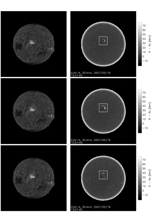
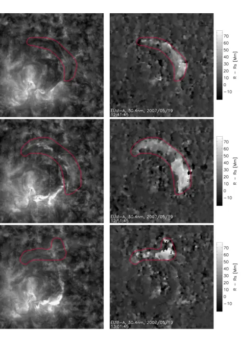
We choose a set of EUVI images observed in 30.4 nm passband observed on 19 May 2007 at times 12:41:45 (top), 12:51:45 (middle) and 13:01:45 (bottom), which have a lossy compression level ICER5. We process them to reconstruct the radius R at each pixel in the image EUVI-A. The stereo separation angle is ∆λ = 8.6 deg.
3.2. Pre-registration: Limb Fitting and Rotation Correction
In order to have correct pointing to the Sun centre, we run the secchi prep.pro IDL routine on a pair of fits images that allows a very high quality pointing. Now images EUVI-A and EUVI-B have their centre pointing to the Sun centre O. We then apply the procedure scc stereopair.pro so that both images the conditions required in Section 2 (see Figure 1). At the end of this pre-registration step, we apply the formula described in Section 2 and Figure 4.
3.3. Displacement Estimation
From the formula (3) we derive the expected displacement between EUVI-A and EUVI-B images. We then apply the Velociraptor algorithm, which gives the displacement at a sub-pixel precision. A high precision is required on the estimation of the upper chromosphere observed in the 30.4 nm passband because the maximum expected height of the maximum network altitude is ≈ 10 Mm above the photosphere altitude (≈ 1.45 % of the solar photospheric radius), while prominences are normally observed in the 10 Mm-100 Mm altitude range.
3.4. Depth Estimation
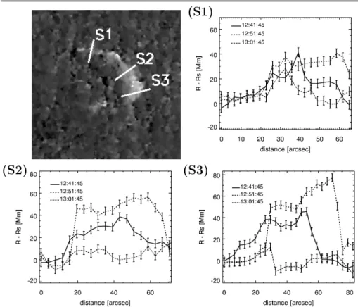
In this particular sequence of 19 May 2007, a filament located in the NOAA active region AR0956 is erupting from frame 12:51:45. The existence of this filament is confirmed by the Hα observation of 19 May 2007 at 06:36:32 provided by the Kanzelh¨ohe observatory (see Figure 7). The GOES flare curve indicates that a C-flare is simultaneously observed in the same active region. At the three different times, we reconstruct the full solar disk; Figure 5 shows the maps of relative radius R. On the left part are the original images, while the radius maps stand in the right column. The dark values, indicating heights below the surface, are due to unstable displacement estimations. In this sequence of three reconstructions, the erupting filament, indicated by a square region of interest (ROI) in the upper right image of Figure 5. The zooms on this ROI are shown in Figure 6. We plot the heights of points located on the filament in Figure 8 and on line segments across the filament in Figure 9. The 1-sigma error bar provided by the formula (10), using a value of σ∆X= 0.5, are overplotted on the height curves. Figures 8
and 9 show the process during which the filament disappears at the same time that a C-flare is observed in the 30.4 nm image (Figure 6, middle and bottom figures); it is confirmed by the GOES flux (Figure 7 (b)). During this sequence of images, the filament is rising and expanding as shown in Figure 9. In the middle image (12:51:45), the flare starts after the onset of the filament eruption. In the lower right figure (13:01:45) of Figure 6, the filament has partially broken away. The brighter part of the ribbons of the flare is situated on both sides of the polarity inversion line (PIL) but only in the part of the PIL where no elevated filament is observed, while a less bright ribbon is observed very closely aligned with the erupting filament, possibly because of the projection effect due to the filament elevation. From our analysis, a possible scenario is that the PIL passes between the two ribbon sites where there is no filament, and that in this part of the PIL, a flare occurs and causes the two ribbons as well as post-flare loops observed in images of hotter coronal lines such as 19.5 nm. Along the part of the PIL where the filament is reconstructed, the eruption occurs without ribbons and post-flare loops because there is no plasma heating in the reconnection site of the erupting filament. In a future work, the filament height estimations will be compared with critical heights of eruption defined and analysed in Filippov and Den, Filippov and Koutchmy (2001, 2002). The time cadence (10 minutes) limits the measurement of the velocity of the erupting filament. Despite this limitation, the present study enables the 3D reconstruction of the on-disc eruption.
Figure 5. Depth map of the EUVI-A stereoscopic reconstruction. Left: original EUVI-A
im-ages observed at times on 19 May 2007 at times 12:41:45 (top), 12:51:45 (middle) and 13:01:45 (bottom). Right: corresponding maps of radius estimations, showing the height R− Rsabove
Figure 6. Depth map of the EUVI-A stereoscopic reconstruction. Left: zoom on original
EUVI-A images observed at times on 19 May 2007 at times 12:41:45, 12:51:45 and 13:01:45. Right: zoom on corresponding maps of radius estimations, showing the height R− Rs above
(a)
(b)
Figure 7. The presence of the filament is also observed in the Kanzelh¨ohe Hα image on 19 May 2007 at 06:36:32 UT in panel (a). The presence of the C-flare is confirmed by the GOES flux in panel (b).
Figure 8. Height above the limb (R− Rs) for pixels 1 to 9.
4. Conclusion
We have presented our method of stereoscopic reconstruction using pairs of EUVI images provided by the two STEREO spacecrafts. We have first established in the heliocentric coordinate system the formula that provides, given the sepa-ration angle and a preprocessing step, the expected displacement between two pixels at the photospheric radius. After inversion of this formula, we derive the stereoscopic reconstruction formula that gives the radius of solar features given the estimated apparent displacement between the two STEREO frames. We use the former formula to calculate the expected displacement at the photospheric level in order to lower the computation time. In the sequence of 19 May 2007, the study of the altitude of the eruptive filament is achieved simultaneously with the observation of a C-flare.
(S1)
(S2)
(S3)
Figure 9. Height variations of segments S1, S2 and S3 above the limb (R− Rs).
In a forthcoming paper, we will process calibration images showing solar-like textures generated on a sphere using the work of Chainais and Li, Chainais (2005, 2007), to calibrate the error prediction method developed in Gissot and Hochedez (2007), and improve the value σ∆X = 0.5 in order to assess with
precision the error on our radius measurement; we expect to be able to measure precisely the local radius of the Sun in the 30.4 nm upper chromosphere, in order for instance to assess the altitude of the chromospheric network. This will also allow us to study the altitude of quiescent and eruptive filaments and their evolution along the year 2007 of STEREO data, and study the mass and 3D motion estimation of the erupting filament.
Acknowledgements The authors acknowledge the support from the Belgian government through ESA-PRODEX. STEREO is a NASA mission. This work has also been supported by a France-Belgium Hubert Curien grant “Tournesol (Communaut´e francophone)”. The Hα image is provided by the Kanzelh¨ohe solar observatory (KSO). We also thanks Andrei Zhukov, Marilena Mierla, and Luciano Rodriguez for fruitful discussions, as well as the anonymous reviewer for his precious comments.
References
Brajˇsa, R., W¨ohl, H., Vrˇsnak, B., Ruˇzdjak, V., Clette, F., Hochedez, J.-F., and Roˇsa, D.: 2004,
Astron. Astrophys., 414, 707
Chainais, P., Li, J.-J.: 2005, In Actes du 20eme colloque GRETSI, Proc. of GRETSI’2005, Presses universitaires de Louvain, 541.
Chainais, P.: 2007, IEEE Transactions On Pattern Analysis and Machine Intelligence, 29. Delaboudini´ere, J.P., Artzner, G.E., Brunaud, J., Gabriel, A.H., Hochedez, J.F., Millier, F., et
al.: 1995, Solar Phys. 162, 291.
Feng, L., Inhester, B., Solanki, S. K., Wiegelmann, T., Podlipnik, B., Howard, R. A., and Wuelser, J.-P.: 2007, Astrophys. J. L., 671, L205.
Filippov, B. P., and Den, O. G.: 2001, J. Geophys. Res., 106, 25177. Filippov, B., and Koutchmy, S.: 2002, Solar Phys., 208, 283.
Gissot, S. F., and Hochedez, J.-F.: 2007, Astron. Astrophys., 464, 1107.
Gissot, S., Hochedez J.-F., Dibos F., Brajˇsa R., Jacques L., Berghmans D., Zhukov A., Clette F., W¨ohl H., and Antoine J.-P.: 2003, In Wilson, A. (ed.), Solar Variability as an Input to
the Earth’s Environment, ESA SP-535, 853.
Inhester, B.: 2006, ArXiv Astrophysics e-prints, arXiv:astro-ph/0612649. Inhester, B., Feng, L., and Wiegelmann, T.: 2007, Solar Phys., 134.
Kaiser, M. L., Kucera, T. A., Davila, J. M., St. Cyr, O. C., Guhathakurta, M., and Christian, E.: 2007, Space Science Reviews, 136, 5.
Lucas, B.D., and Kanade, T.: 1981, Proc. of the 7th International Joint Conference on
Artificial Intelligence (IJCAI ’81), 674.
Rosa, D., Vrsnak, B., Bozic, H., Brajsa, R., Ruzdjak, V., Schroll, A., W¨ohl, H.: 1998, Solar
Phys. 237, 179.
Vrˇsnak, B., Roˇsd, A., Boˇzi´c, H., Brajˇsa, R., Ruˇzdjak, V., Schroll, A., W¨ohl, H.: 1999, Solar