HAL Id: hal-00318007
https://hal.archives-ouvertes.fr/hal-00318007
Submitted on 19 May 2006
HAL is a multi-disciplinary open access
archive for the deposit and dissemination of
sci-entific research documents, whether they are
pub-lished or not. The documents may come from
teaching and research institutions in France or
abroad, or from public or private research centers.
L’archive ouverte pluridisciplinaire HAL, est
destinée au dépôt et à la diffusion de documents
scientifiques de niveau recherche, publiés ou non,
émanant des établissements d’enseignement et de
recherche français ou étrangers, des laboratoires
publics ou privés.
time-varying magnetic reconnection: III.
Quasi-instantaneous convection responses in the
Cowley-Lockwood paradigm
S. K. Morley, M. Lockwood
To cite this version:
S. K. Morley, M. Lockwood. A numerical model of the ionospheric signatures of time-varying
mag-netic reconnection: III. Quasi-instantaneous convection responses in the Cowley-Lockwood paradigm.
Annales Geophysicae, European Geosciences Union, 2006, 24 (3), pp.961-972. �hal-00318007�
www.ann-geophys.net/24/961/2006/ © European Geosciences Union 2006
Annales
Geophysicae
A numerical model of the ionospheric signatures of time-varying
magnetic reconnection: III. Quasi-instantaneous convection
responses in the Cowley–Lockwood paradigm
S. K. Morley1,*and M. Lockwood1,2
1School of Physics and Astronomy, University of Southampton, UK
*also at: CRC for Satellite Systems, University of Newcastle, NSW, Australia 2Rutherford Appleton Laboratory, Chilton, Oxfordshire, UK
Received: 7 October 2005 – Revised: 18 January 2006 – Accepted: 13 March 2006 – Published: 19 May 2006
Abstract. Using a numerical implementation of the
Cow-ley and Lockwood (1992) model of flow excitation in the magnetosphere–ionosphere (MI) system, we show that both an expanding (on a ∼12-min timescale) and a quasi-instantaneous response in ionospheric convection to the onset of magnetopause reconnection can be accommodated by the Cowley–Lockwood conceptual framework. This model has a key feature of time dependence, necessarily considering the history of the coupled MI system. We show that a resid-ual flow, driven by prior magnetopause reconnection, can produce a quasi-instantaneous global ionospheric convection response; perturbations from an equilibrium state may also be present from tail reconnection, which will superpose con-structively to give a similar effect. On the other hand, when the MI system is relatively free of pre-existing flow, we can most clearly see the expanding nature of the response. As the open-closed field line boundary will frequently be in motion from such prior reconnection (both at the dayside magneto-pause and in the cross-tail current sheet), it is expected that there will usually be some level of combined response to day-side reconnection.
Keywords. Ionosphere (Modeling and forecasting; Plasma
convection) – Magnetospheric physics (Magnetosphere-ionosphere interactions)
1 Introduction
1.1 Observations of expanding and quasi-instantaneous convection responses
There are seemingly conflicting views on how the iono-spheric convection pattern responds to a change in the ap-plied reconnection. The first observation of an evolving
Correspondence to: S. K. Morley
(steven.morley@newcastle.edu.au)
ionospheric response to magnetopause reconnection was made by Lockwood et al. (1986) who correlated IMF data from the AMPTE-UKS (Active Magnetospheric Particle Tracer Explorer – U.K. Satellite) with ion temperature mea-surements from EISCAT. They found that the observed ion temperature enhancement propagated away from noon with a mean velocity of 2.6±0.3 km s−1. Other studies, for exam-ple, the case study by Saunders et al. (1992) and the statisti-cal surveys by Todd et al. (1988), Etemadi et al. (1988) and Khan and Cowley (1999) all reported this expansion, which was combined with ideas on boundary motions and flows dis-cussed previously by Siscoe and Huang (1985) and Freeman and Southwood (1988) in the model of the ionospheric flow response proposed by Cowley and Lockwood (1992). The Cowley–Lockwood model invokes an equilibrium state that the near-Earth system will approach with the cessation of re-connection. As the system approaches equilibrium the flows will die away, even if open flux is still present. Subsequent reconnection at the magnetopause or in the tail will perturb the system away from equilibrium and excite flow which car-ries the system towards a new equilibrium for the changed amount of open flux. Under an applied change in magneto-pause reconnection, convection will first respond locally on the dayside, before evolving around the flanks and into the nightside (Cowley and Lockwood, 1997).
The view of an expanding reconfiguration of the con-vection flow pattern, interpreted in the framework of the Cowley–Lockwood model, was challenged by Ridley et al. (1998). Their study used a global assimilative mapping tech-nique (AMIE, Richmond and Kamide, 1988) to generate pat-terns of electrostatic potential from magnetometer data. A method of producing residual potential patterns, subtracting an initial potential map from subsequent potential maps, was developed to show the deviation from the initial potential pat-tern. They interpreted their results as showing a globally in-stantaneous response, within the temporal resolution of their data, and thus concluded that this was inconsistent with the
Cowley–Lockwood model. Ruohoniemi and Baker (1998) used another large-scale technique to observe the convection response to variations in the IMF. Using the Doppler shift of observed coherent radar echoes from the SuperDARN radar network, these authors then used the line-of-sight velocities to constrain a mathematical fitting of an electrostatic poten-tial pattern. Where insufficient data is gathered for a spheri-cal harmonic fit of a given order, data from a statistispheri-cal model (the APL model, see Ruohoniemi and Baker (1998) and ref-erences therein) is used to augment the measurements. The same technique was used by Ruohoniemi and Greenwald (1998) for a more detailed examination of one of the peri-ods used as a case study in Ruohoniemi and Baker (1998). These studies also concluded that the ionospheric convection pattern responded globally simultaneously to a change in the applied reconnection voltage.
In a comment on the Ridley et al. (1998) paper, Lockwood and Cowley (1999) argued that the data presented by Rid-ley et al. (1998) in fact showed an expansion commensu-rate with the timescales for reconfiguration inferred by the prior, directly-measured studies. They also raised an impor-tant point regarding the distinction between the convection change and the shape of the convection pattern. A recent review by Ruohoniemi et al. (2002) highlighted some fur-ther shortcomings of using global mapping procedures (e.g. AMIE). These authors reached the conclusion that global as-similative techniques have a tendency to “globalize” local be-haviour. They noted that the integration of statistical model data into the solution can also tend to globalize the effects of a local disturbance. They considered the case of a localized velocity vortex and reasoned that in the absence of sufficient data coverage in the surrounding area, the solution for the global potential pattern would adjust itself to accommodate a greater convective flow.
1.2 Numerical modelling of time-dependent convection Further to this discussion, it should be noted that using sta-tistical averages for a quasi-steady state goes against the paradigm of a time-varying response to convection. Con-sider the usage of a global assimilative method in the case of data coverage only in one quadrant of the hemisphere. The statistical model used, (e.g. the APL model, Ruohoniemi and Baker, 1998), will supply averaged data corresponding to a fixed IMF orientation. This data corresponds to a quasi-steady (or “equilibrium”) condition, and does not consider the history of the magnetosphere–ionosphere system. By presupposing and adding in the equilibrium (final) state to a reconfiguring (intermediate) state, the global mapping pro-cedure may artificially show a more instantaneous response. Thus caution must be exercised when interpreting data that has been “filled in” with statistical data.
Freeman (2003) described both the expanding and instan-taneous responses within a single mathematical framework of the expanding-contracting polar cap (ECPC) model. His
results showed that the expanding response fitted the obser-vations better and that examining the convection patterns, the technique used by Ridley et al., made it hard to differenti-ate between the competing models. The expanding solution found by Freeman had the peaks of the convection pattern expanding around the polar cap boundary, but the entire equi-librium boundary was allowed to respond instantaneously. This form of expanding solution is consistent with the ini-tial conceptual picture put forward in Cowley and Lock-wood (1992), as shown in their Fig. 5. However, in later pa-pers (Cowley and Lockwood, 1997; Lockwood and Cowley, 1999) these authors noted that the equilibrium boundary per-turbation would expand tailward as newly-opened flux was added to the tail (see Figs. 2 and 3 of Lockwood and Mor-ley, 2004). The numerical model of Lockwood and Morley (2004), hereafter Paper 1, goes beyond the Freeman (2003) model by taking these later ideas fully into account. While the high-latitude ionosphere can have a change in potential communicated across it on a timescale of tens of seconds by means of a fast Alfv´en wave (Freeman et al., 1991; Ruo-honiemi and Greenwald, 1998), the change in potential (as-sociated with the development of new region 1 and region 2 field-aligned current (FAC) systems) may take time to de-velop.
1.3 Two-stage ionospheric convection response
Using magnetometer data, Murr and Hughes (2001) found that the onset of change occurred globally on timescales of about 2 min – a similar timescale to that reported by Rid-ley et al. (1998). However, their study also showed that the subsequent reconfiguration took place as a function of local time. The timescale for this reconfiguration was, on average, 10 min for complete reconfiguration of the ionospheric con-vection pattern – a result similar to those reported by Lock-wood et al. and co-workers. There have been a number of other observations of a two-stage response in ionospheric convection reported in the literature. Jayachandran and Mc-Dougall (2000) used two digital ionosondes to study the po-lar cap convection change associated with southward turn-ings of the IMF and reported both a quasi-instantaneous and an expanding response. Combined observations of the po-lar cap using SuperDARN radars and ground magnetometers were presented by Nishitani et al. (2002) and Lu et al. (2002). These authors found that the ionospheric flow vortices re-sponded initially within the temporal resolution of their in-struments, whereas the polar cap boundary and peak mag-netic perturbation responded with a delay of up to 25 min. Lu et al. (2002) inferred that the two-stage response was a consequence of several interacting processes, including a fast rarefaction wave in the magnetosphere and a fast mag-netosonic wave in the ionosphere. They also argued that the most important process was the feedback between the iono-sphere and magnetoiono-sphere. The propagation of a fast magne-tosonic wave as the cause of fast onset of change in response
to a change in reconnection was also cited by Nishitani et al. (2002).
Lopez et al. (1999) showed in their three-dimensional MHD simulation that the convection pattern across the en-tire polar cap begins to change a few minutes after the arrival of the southward IMF, whereas the onset of the equatorward motion of the open-closed field line boundary depends on the local time, with equatorward motion of the midnight bound-ary delayed by ∼20 min relative to the onset of the boundbound-ary motion at noon. The MHD modelling study of Slinker et al. (2001) also found a fast onset of change in the ionospheric convection with a slower reconfiguration. The fast response was attributed to the propagation of a fast magnetosonic wave through the magnetosphere.
Using a numerical implementation of the Cowley– Lockwood paradigm, Lockwood and Morley (2004) showed that a quasi-instantaneous response could occur alongside the expected expansion, to an extent that depended on the level of pre-existing flow before the change. This paper will show how the Cowley–Lockwood (1992; 1997, hereafter CL) con-ceptual framework can accommodate a quasi-instantaneous response, demonstrated with the numerical model of Lock-wood and Morley (2004). That the CL paradigm could ac-commodate this kind of response was noted in Paper 1, but was not studied in detail. In this paper we examine this effect using the Lockwood-Morley numerical model with an input reconnection rate variation having two identical pulses sepa-rated in time and making use of the techniques developed by Morley and Lockwood (2005, hereafter Paper 2).
2 The Lockwood-Morley numerical model
Lockwood and Morley (2004) presented a novel numerical model of the ionospheric convection response to variations in reconnection rate, incorporating all the concepts of the CL paradigm. The numerical model uses non-circular polar cap and equilibrium boundaries, and includes the propagation of a perturbation in the open-closed field line boundary (OCB). A full description of the model, its assumptions and limita-tions can be found in Paper 1. Paper 2 extended the model to calculate the ionospheric ion temperature and used the model to analyse the accuracy of the various methods used to derive expansion effects from experimental data. In this section we will outline the basic features of the model which are relevant to the expansion of the simulated flow patterns. For further details the reader is referred to Papers 1 and 2.
The model calculates the temporal evolution of the OCB and the equilibrium boundary latitudes, 3OCBand 3E, at all
magnetic local times. At any point in this temporal develop-ment of the boundaries, various outputs can be derived. A flowchart summary of the operation of the model can be seen in Fig. 1 of Paper 2.
The basic operation of the numerical model relies on three types of input: the input reconnection rate (ε) variation, the
initial conditions of the model high-latitude ionosphere and the constants assumed for the return of the OCB to equilib-rium.
We first define the convection velocity across the boundary (V0), in its own rest frame, for a given time. The latitudinal convection velocity at the boundary (Vcn) is then calculated
and the latitudinal velocity of the OCB (Vb) is determined.
Thus the latitude of the OCB (3OCB) is defined at all MLT
for any given simulation time, ts. The equilibrium
bound-ary latitude (3E) is then updated as a function of MLT to
accommodate the new amount of open flux contained within the polar cap. The speed at which the perturbation to the equilibrium boundary propagates antisunward is the limit to the expansion of response of the OCB, and hence to the ex-pansion of the convection pattern. The simulation time is then advanced and the input reconnection rate for the current model timestep updated. These steps then repeat for each simulation time.
The latitudinal convection velocity is used to specify the distribution of electric potential around the polar cap bound-ary. Using the ionospheric convection solution given in Free-man et al. (1991) and FreeFree-man (2003) for a circular OCB, the instantaneous convection velocity for all points in the modelled high-latitude ionosphere is specified for any given timestep. Perturbation analysis is used to allow for depar-tures of the OCB from a circular form. As in Paper 2 the ion temperature at a series of simulated stations at a constant latitude is calculated for each timestep. As there is a sym-metry about the noon-midnight meridian, we employ a lati-tudinal ring of 72 simulated stations in the dawn hemisphere (at 67◦; i.e. outside the polar cap), with a spacing in MLT of 10 min. Note that the polar cap is centred on a latitude of 90◦ in the frame used and not offset towards the nightside as in a conventional geographic or geomagnetic frame. Therefore, using a latitudinal ring in this frame ensures that the (equilib-rium) OCB is equidistant from the stations at all MLTs. This allows us to isolate the azimuthal expansion of the convection pattern and avoid mixing it with any latitudinal expansion.
3 Modelling the response to pulsed reconnection
Paper 2 presented an examination of how using cross-correlation methods and threshold techniques can influence the observed convection response to IMF changes in time-series data. It was concluded that the most reliable method of recovering the expansion of the onset of the convection response is to use time series data with a threshold that is a fixed fraction of the peak response.
The first pulse of reconnection in the simulation presented in this paper is exactly identical to that used for the exam-ple of model results discussed in Paper 2. A second, iden-tical, pulse of reconnection is added here, commencing at
ts =540 s, 8 min after the commencement of the first pulse.
0 450 900 1350 1800 0 20 40 t s = 540s ΦPC ΦXL/ 5 kV ΦPC = 16 kV Φ XL = 0 kV F PC = 8.17 x 10⁸ Wb ΔΦ = 3 kV 60 deg 12 MLT = 0hrs 18 6
Fig. 1. A model output convection pattern for ts=540 s, just prior to
the activation of the second pulse of magnetopause reconnection. At this point the convection from the first applied pulse of reconnection has started to decay. The top panel shows the variation with simu-lation time, ts, of the input reconnection voltage (in blue), 8XL di-vided by five to fit the same scale as the resulting transpolar voltage (in red), 8P C. The vertical green line marks the simulation time of the output frame. The lower panel shows the convection pattern (using equipotentials 3 kV apart) plotted in an MLT–magnetic lati-tude coordinate system. The outer circle represents the equatorward boundary of the modelled region (i.e. the region 2 FAC ring) and the inner circle represents the OCB. Non-reconnecting segments of the OCB are shown in black (in this case no reconnection is ongoing and so the entire OCB is black). The green line delineates the re-gion of newly-opened flux produced by the first reconnection pulse. The open flux at this ts is FP C=8.17×10⁸Wb, showing that the first pulse added 1.7×10⁷Wb of open flux.
period of magnetopause flux transfer events (Rijnbeek et al., 1984; Lockwood and Wild, 1993). The simulation com-mences with a total open flux of FP C=8×10⁸Wb. Each
reconnection pulse starts at the X-line centre and expands towards both dusk and dawn (to the points a and b, respec-tively) at a rate (d|φX|/dts)which we set to 0.167◦s−1,
cor-responding to 1 h of MLT per 1.5 min. Similarly, the end of each reconnection pulse is first seen at 12:00 MLT, t =1 min after the onset, and propagates towards both a and b at the
s
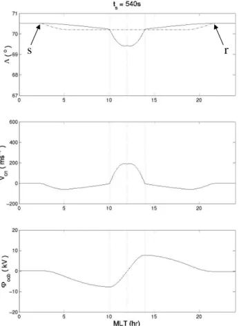
r
Fig. 2. Model output boundary characteristics corresponding to Fig. 1. The top panel shows the latitude as a function of MLT, of the OCB (solid line), 30, and the equilibrium boundary (dash-dot line), 3E. The middle panel shows the poleward convection velocity at the OCB, Vcn, caused by the motion of the boundary. The bottom panel shows the electrostatic potential around the OCB, 8OCB. The vertical dashed line in each panel marks the centre of the merging gap, at 12:00 MLT, and the dotted lines mark the maxi-mum extent of the merging gap. These lie at 10:00 and 14:00 MLT. Note that the perturbation to the equilibrium boundary has propa-gated to the points marked s and r.
same rate. Thus each pulse causes the reconnection to be active at any MLT between a and b for 1 min. Two such pulses are included in the present simulation, with onsets at
ts=1 min and ts=9 min. The background reconnection rate
outside the two pulses is taken to be zero.
A constant reconnection electric field of 0.2 V m−1is ap-plied at each MLT of the ionospheric projection of the X-line for 1 minute, expanding from noon MLT to cover a maxi-mum X-line extent of 4 h of MLT. This azimuthal movement of the active reconnection region is as proposed and deduced from observations by, e.g., Lockwood et al. (1993a), Milan et al. (2000) and McWilliams et al. (2001). The model re-sponse is identical to that presented in Paper 2 until the com-mencement of the second pulse. The effects of an existing flow-pattern (that is, a disturbed OCB) caused by the first
0 450 900 1350 1800 0 20 40 t s = 600s ΦPC ΦXL/ 5 kV ΦPC = 20 kV Φ XL = 158 kV F PC = 8.22 x 10⁸ Wb ΔΦ = 3 kV 60 deg 12 MLT = 0hrs 18 6
Fig. 3. A model output convection pattern for ts=600 s, 60 s after
the commencement of the second pulse of reconnection. The format is the same as Fig. 1. Active segments of the OCB, which map to the magnetopause X-line where reconnection is ongoing, are shown in red.
pulse on the model response to the second pulse are discussed below.
Prior to the onset of the second pulse of reconnection, the flows generated by the initial pulse of reconnection have not yet subsided and the convection pattern at simulation time
ts=540 s is shown in Fig. 1. A full sequence of flow pattern
plots for a similar reconnection scenario to that employed here is given in Paper 1.
At this time the second pulse of reconnection is about to commence. The convection pattern is diminishing in strength while the extent of the pattern continues to grow over the po-lar region. The upper panel of Fig. 1 shows the variation with simulation time, ts, of the input reconnection voltage, 8XL(in blue), divided by five. It can be seen that the
re-connection pulses are spaced 8 min apart and that they are identical. The polar cap voltage, 8P C(in red), has already
peaked at about 18 kV by this time and has subsequently de-cayed slightly – this is shown in the presence of only 3 plot-ted equipotentials, which are separaplot-ted by 3 kV and centred about zero. The boundary locations for this time are shown
s
1r
1r
2s
2a
b
Fig. 4. Model output boundary characteristics corresponding to Fig. 3. The format is the same as Fig. 2. r1and s1mark the ex-tent of the perturbation to the equilibrium boundary (dash-dot line) caused by the first pulse of reconnection. Similarly, r2and s2mark the extent of the perturbation to the equilibrium boundary due to the second reconnection pulse. The extent of the active OCB (the active “merging gap”, mapping to the segment of the magnetopause where reconnection is ongoing – solid line) is between the points a and b. The middle and lower panels show the poleward convection velocity at the OCB and the electrostatic potential around the OCB, respectively.
in Fig. 2 (top panel), along with the convection velocity in the boundary rest frame (middle panel) and the electrostatic potential along the OCB (lower panel).
The equilibrium boundary perturbation – the point at which the OCB can have responded to the added open flux – has propagated beyond 03:00 and 21:00 MLT (points s and r) on the dawn and dusk sides respectively. The poleward flow between 10:00 and 14:00 MLT (the maximum extent of the merging gap) is balanced by the equatorward flow outside of this region.
Figure 3 shows the convection pattern at ts=600 s. This
shows the model output 60 s after the initiation of the second pulse of reconnection. The actively reconnecting segments of the merging gap are shown by the thick red lines. The green lines delineate the regions of newly-opened flux formed by
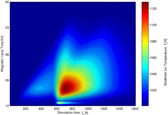
Fig. 5. A formedogram of the amplitude of the ion temperature response to the series of two reconnection pulses. The plot colour-codes the ion temperature as a function of simulation time ts(horizontal axis) and magnetic local time (vertical axis: where 00 MLT corresponds to simulated station number 72 and 12:00 MLT corresponds to simulated station 0; all stations are at a latitude of 67◦). This plot is the same as Fig. 6 of Morley and Lockwood (2005), but with a second burst of reconnection, identical to the first, 8 min after the commencement of the first. Note the change in the ion temperature scale compared with that used by Morley and Lockwood (2005), which is required because much higher temperatures are driven in response to the second pulse.
each reconnection pulse. The ionospheric merging gap volt-age is at its peak of 8XL=158 kV and the transpolar voltage, 8P C, has risen from 16 kV to 20 kV (but does not reach its
peak value of near 30 kV until 150 s later).
Figure 4 shows the boundary characteristics at ts=600 s in
the same format as Fig. 2. The latitudes of the OCB (solid line) and equilibrium boundary (dash-dot line), as a function of MLT, are shown in the upper panel. A boundary erosion identical to that caused by the first pulse is superimposed on the already distorted boundary. This new bulge is bounded by points a and b. The extent of the equilibrium boundary perturbation to the second pulse is marked by points r2and s2, while the corresponding limits for the perturbation due
to the first pulse, r1 and s1, have expanded to nearer
mid-night compared with Fig. 2. The middle panel shows Vcnhas
increased by a substantial amount between a and b. This in-crease is not balanced (as it was at the same stage for the first pulse) by equatorward flow between both a and r2and b and s2. Comparison of the lower panel with Fig. 2 shows that the
potential around the OCB is enhanced everywhere between
r1and s1.
Figure 5 shows the formedogram (from the Greek
formedon – meaning “in layers crosswise”) for the ion
temperature enhancement resulting from this two-pulse re-connection variation. This format show the contours of the ion temperature enhancement, resulting from the enhanced ion flow, as a function of simulation time, ts, and
mag-netic local time, where 12:00 MLT corresponds to station 0. The simulated stations are at a latitude of 67◦and are posi-tioned around the dawn hemisphere with a spacing in MLT of 10 min. We have examined the effect of the initial pulse of reconnection in isolation in Paper 2. This first pulse of reconnection produces convection in the model, as the OCB responds to displacement from its equilibrium configuration. When the second pulse of reconnection is applied, the con-vection resulting from the first pulse is still present. Although the response in ion heating to the first pulse is identical to that presented in Paper 2, comparison of Fig. 5 with Fig. 7 of Paper 2 highlights the difference in the level of the re-sponse to the second pulse. This is also apparent from Fig. 5 alone when one compares the initial response to reconnec-tion pulses 1 and 2, the maximum simulated ion tempera-ture reaching over 1120 K. This is significantly larger than the peak of about 1040 K in response to the first reconnec-tion pulse. The temperature anomaly in the data series for simulated station 3 ('11:30 MLT) is not an erroneous point:
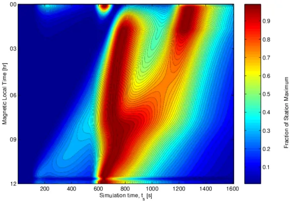
Fig. 6. Same as Fig.5, but normalized to the maximum response at each simulated station. Contours of (Ti–Ti0)/(Tp–Ti0) are plotted as a function of MLT and simulation time, ts, where Ti0is the value of Tiat ts=0 and Tipis the peak temperature seen at that station during the simulation.
it arises from the proximity of the active reconnection X-line footprint and was discussed in Paper 2. This is the only sta-tion to be engulfed by the temperature enhancement that is localized around the end of the merging gap.
Figure 6 shows the ion heating response (as a function of both simulation time, ts, and MLT) by presenting the ion
temperature change for each MLT, normalized to the local peak change at that MLT. For the first pulse, the response is weaker at all MLT and shows a clear anti-sunward propaga-tion, with the enhancement being later at larger virtual station number (i.e. at MLT increasingly removed from noon). How-ever, the (larger) response to the second reconnection pulse shows both a quasi-instantaneous response and an expanding response. The character of the response varies with MLT. The apparently instantaneous response present near midnight is due to numerical noise (of order 0.1 K) being amplified by the normalization as described in Paper 2. Visual compari-son with Fig. 5 shows that the amplitude of the temperature change is negligible.
The two reconnection pulses are identical and the differ-ence in response to the two highlighted by Figs. 5 and 6 reveals that the effect of a pre-existing background flow is substantial. Equivalently, localized addition of open flux to a non-equilibrium polar cap can cause a large-scale response. This will be explained in the following section.
4 Discussion
We have presented results from the Lockwood and Morley (2004) numerical model predicting the effect of superposing a reconnection pulse on both an undisturbed and an already-disturbed ionosphere. The inputs to the model are identical to those presented in Paper 2, with the exception of the in-put reconnection rate which now includes a second, identi-cal, pulse of reconnection commencing at ts=540 s, 8 min
after the commencement of the first reconnection pulse. The convection patterns presented in Figs. 1 and 3 (for
ts=540 s and 600 s, respectively) appear to show a global
in-crease in convection strength in response to the second of the two applied reconnection pulses. For the first pulse (perturb-ing an undisturbed MI system) the effect is initially localised around the reconnection site, but then expands. The second pulse (perturbing an MI system that has already been per-turbed by the first pulse) has a larger response which has both instantaneous and expanding characteristics (as revealed by Fig. 6). The principles of this effect can be understood from Fig. 4. The top panel shows the latitudes of both the OCB,
3OCB, and the equilibrium boundary, 3E, as functions of
MLT. The perturbation to the equilibrium boundary caused by the first reconnection pulse has almost reached 23:00 MLT on the dusk side (r1) and near 01:00 MLT on the dawn
response to the first pulse of reconnection. This perturbation due to the first pulse is close to encircling the polar cap, al-lowing the entire OCB to respond, and thus in the absence of the second pulse the convection pattern would have decayed exponentially in a quasi shape-preserving manner (see Pa-per 2). However, the Pa-perturbation to the equilibrium bound-ary caused by the addition of new open flux to the polar cap is initially confined to the reconnection site with a subsequent expansion at a velocity dφr2/dts, with point r2propagating
eastward away from a and s2 propagating westward away
from b. This is exactly the same perturbation motion expe-rienced by the equilibrium boundary in response to the first pulse of reconnection.
The residual effect of the first pulse can be seen in the OCB latitude by the fact that it has migrated equatorward at MLTs outside the merging gap (except near midnight, where nei-ther 3Enor 3OCB have yet been influenced). However, the
OCB is still poleward of its equilibrium position everywhere outside the ionospheric footprint of the X-line (the “merg-ing gap”). The effect of the second pulse can be seen as a large equatorward migration within the active merging gap
ab. The effects of the two pulses can be also be distinguished in the poleward convection speeds, with equatorward motion (Vcn<0) at MLTs outside the merging gap (except near
mid-night) and strong poleward flow (Vcn>0) inside the merging
gap. An enhancement of the equatorward flow is seen just outside of the merging gap (between a and r2and between b and s2), but this is much weaker than the poleward flow
between a and b. This should be contrasted with the situa-tion for the equivalent time following the first pulse (Fig. 4 in Paper 1) where the total equatorward flow (between a and
s1and between b and r1) matches the total poleward flow
be-tween a and b: this is the case for all times when a zero-flow equilibrium system is perturbed by a single pulse of recon-nection and can also be seen in Fig. 2. Indeed, in the bottom panels of Figs. 2 and 4 it can be seen that the additional equa-torward flow between a and s2and between b and r2causes
only a very small perturbation to the potential distribution around the OCB.
In the CL model the displacement from equilibrium is what determines the flow normal to the OCB at a given loca-tion. Where the OCB is close to the equilibrium boundary, only weak flow will be excited. In this example the OCB and equilibrium boundary are close together at s2and r2, hence |3OCB−3E|is small and Vcn is near zero. This situation
arises because the equilibrium boundary at these MLTs is perturbed equatorward by the second pulse of reconnection. However, the OCB has been eroded equatorward by a similar amount in response to the first pulse. In the absence of the perturbation due to the first pulse the streamlines would re-turn across the OCB sunward of s2and r2. Near these points
at this simulation time, ts=600 s, the flow that would have
been caused by the first pulse in isolation is poleward and comparable in magnitude to the equatorward flow that would result from the second pulse in isolation. They can thus be
considered to cancel each other out here, and the equator-ward flow required because the ionosphere is incompressible must take place elsewhere (between r1and r2and between s1and s2, i.e. closer to midnight). The flow increases at all
MLTs between s1and r1. It is important to note that the flows
do not superpose – rather it is the boundary perturbations that superpose and their subsequent return towards their equilib-rium position governs how the flow responds.
This “global” strengthening of the convection pattern may provide an explanation for the quasi-simultaneous response reported by several authors (e.g. Ridley et al., 1997; Ruo-honiemi and Baker, 1998). In this context, it is useful to note that Ridley et al. studied perturbations to the flow in response to southward turnings of the IMF using “residual potential patterns”. These were obtained by subtracting from each ob-served potential a pre-existing potential from before the IMF change. Thus in their examples there was pre-existing flow as in the simulation presented here.
4.1 Ion temperature response
As described in Paper 2, the convection response is also clearly seen in the ion heating – the dependence of ion heating on the convection velocity approximately follows a squared relationship (we here neglect the effects of thermo-spheric neutral winds and their (slow) response to the convec-tion change). The formedogram of simulated ion temperature (as a function of simulation time and MLT) shown in Fig. 5 reveals response to the first pulse of reconnection which, as in Paper 2, expands away from noon at about 11 km s−1. The second pulse of reconnection commences at ts=540 s. The
erosion of the OCB is almost identical to that caused by the first pulse of reconnection applied. However, the response in the ion heating reveals a very different convection response. The response in frictional ion heating, hence in the convec-tion, appears in Fig. 5 to be nearly simultaneous across the entire dayside. However, as discussed earlier, observing at a fixed threshold level can lead to a significantly reduced ap-parent expansion velocity and to a reduced apap-parent extent of the expansion. This formedogram also shows a bifurcation in the response to the second pulse, with an apparent expanding component in addition to the more instantaneous response.
Figure 6 shows the ion heating response (as a function of simulation time and MLT), where the data from each simu-lated station has been normalized to the local maximum – i.e. the contours represent the fraction of peak change in ion tem-perature at a given MLT. Here the effect of the reconnection onset just after ts=540 s is clearly seen globally, with a rise
to peak convection response within 3 min of the commence-ment of addition of open flux by the second pulse of recon-nection. Only on the nightside is there any evidence for an antisunward expansion of this quasi-instantaneous response. This interaction between the flow present prior to the second pulse and the new flow, giving the global response, then falls away and a second, expanding, response can be seen moving
Fig. 7. Same as Fig.5, but for a reconnection pulse separation of 10 min. Note the change in the ion temperature scale used compared to Fig. 5 because lower temperatures are driven by the second pulse; this results from the greater separation between pulses allowing the remnant flow to decay further.
anti-sunward with a similar phase velocity to that for the first pulse, i.e. with a velocity of about 11 km s−1. The peak ion heating response at 00:00 MLT is seen to occur at ts=1250 s,
about 12 min after the onset of the second reconnection pulse, corresponding to the timescale for reconfiguration of the en-tire convection pattern. The temporal separation between the two responses becomes sufficiently large that we can sepa-rate them as we approach the dawn-dusk meridian. It is in-teresting to note that in this case the expanding response is of lesser magnitude than the quasi-instantaneous response, as measured by the ion heating, falling as low as 70% of the peak response at some MLTs.
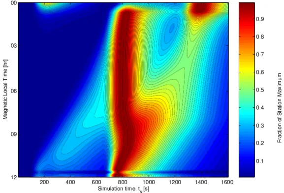
4.2 The effect of pulse separation
To illustrate the effect of the separation between reconnec-tion pulses on the quasi-instantaneous and expanding re-sponses we here use the input reconnection scenario de-scribed earlier in this paper, but increase the separation be-tween the applied pulses of reconnection to 10 min; i.e. the second pulse of reconnection now commences at ts=660 s.
The formedograms of simulated ion temperature for this case are shown in Figs. 7 and 8 (corresponding to Figs. 5 and 6, respectively).
Comparison of Fig. 7 with Fig. 5 shows that the form of the response in ion temperature is qualitatively similar. Since the reconnection pulses have a greater separation in time, the
flow excited by the initial pulse of reconnection has decayed further at the onset of the second pulse. The response to the second pulse is therefore slightly lower in magnitude than in the previous example.
Figure 8 shows the effect of the increased pulse separa-tion on the heating, as a fracsepara-tion of the maximum response at each station. As before, the quasi-instantaneous response is present across much of the high-latitude ionosphere. Here the onset of the ion heating response occurs over a greater MLT extent than before, and no longer shows the antisun-ward expansion of the quasi-instantaneous response present in Fig. 6. This global strengthening of the ionospheric con-vection again shows the greatest perturbation in the temper-ature profiles for each simulated station. This is explained by the fact that the expanding response, which is smaller in this example because of the greater pulse separation, weak-ens as it spreads around the auroral oval towards the night-side. It therefore has less effect on the magnitude of the change in convection, and the resultant ion heating. This can be seen in the different ion temperatures just after the onset of the second reconnection pulse. For the case of an 8-min separation the peak temperature measured here is 1125 K, whereas for a pulse separation of 10 min the peak temper-ature around 10 K lower. However, the heating associated with the quasi-instantaneous response covers a larger MLT extent. The decay of the instantaneous response is with the
Fig. 8. Same as Fig.6, but for a reconnection pulse separation of 10 min.
same time constant as that for the decay of the residual flow associated with the first pulse (of order 10 min).
The superposed and expanding responses are still diffi-cult to distinguish on the dayside, where the simulated ion temperature increase is greatest. However, on the dayside the response to an applied pulse of reconnection is observed in the ion heating as a temperature enhancement expanding away from the reconnection footprint. In these examples the quasi-instantaneous strengthening of the convection pattern, as seen in the associated ion heating, can only be fully sep-arated from the classic Cowley–Lockwood (1992; 1997) ex-panding response on the nightside.
For small pulse separations, the instantaneous response will not be seen as the two reconnection pulses effectively merge into a single, longer-lived pulse. Comparison of Figs. 5 and 7 illustrates how the magnitude of the instanta-neous response in ion heating decays with increasing pulse separations above 8 min, eventually disappearing to leave two identical expanding responses of the type presented in Paper 2.
5 Conclusions
We have shown that both expanding (on a ∼12-min timescale) and quasi-instantaneous responses of the iono-spheric convection to magnetopause reconnection can be ex-plained with the Cowley and Lockwood (1992, 1997) model of flow excitation in the coupled magnetosphere–ionosphere
(MI) system. This model has a key feature of time-dependence, necessarily considering the prior history of the MI region. The work presented in this paper shows that a residual flow from magnetopause reconnection can produce a quasi-instantaneous global ionospheric convection response; residual flow may also be present from tail reconnection, which will superpose constructively to give a similar effect. The flow generated by the second pulse is not a simple super-position of the flow patterns associated with the two pulses in isolation. Rather, it is the boundary perturbations (the OCB and equilibrium boundary) which are superposed and the combined effect of the two pulses gives a quite different response to the isolated patterns or the superposition of the two as the OCB migrates back towards its equilibrium posi-tion.
As the OCB will frequently be in motion from such prior reconnection (both at the dayside magnetopause and at a magnetotail neutral line), it is expected that there will usually be some level of combined response to dayside reconnection. IMF By and its variations will also have an effect, though
modelling of the effect of a strong Bycomponent cannot be
achieved with the current model, since symmetry is assumed in the analytic solution of Laplace’s equation.
The example presented offers a plausible explanation for reported global responses within the Cowley–Lockwood paradigm. The model predicts a quasi-instantaneous strengthening of the convection pattern along with the ex-pected expanding reconfiguration response, in accordance
with observations by, for example, Murr and Hughes (2001) and Lu et al. (2002). Note that these responses in our mod-elling are not due to the presence of different magnetosonic wave speeds. Other mechanisms have been proposed to ex-plain certain cases, including an overdraped lobe causing re-connection onset simultaneously across a large MLT extent (e.g. Shepherd et al., 1999). However, our results show that these are also not necessary to explain the observations.
In the sample results presented, the “global” and “expand-ing” responses in the bulk flow occurred too close together to be separated across much of the dayside. The reconfigura-tion of the ionospheric flows in response to the applied pulse of reconnection is seen to occur as an expanding reconfigura-tion of the type discussed by Cowley and Lockwood (1992). Further, the separation between dayside reconnection events, is seen to be an important factor in the degree of separation between the global and expanding responses, and in the level of the quasi-instantaneous response caused by the superpo-sition of the OCB and equilibrium boundary perturbations. In the present paper we have concentrated on the effects of pulses in the magnetopause reconnection rate; however, sim-ilar effects will also be produced by pulses in the nightside reconnection in the cross-tail current sheet.
Acknowledgements. This work was supported by the UK Particle
Physics and Astronomy Research Council and the Cooperative Re-search Centre for Satellite Systems through the Commonwealth of Australia CRC Program.
Topical Editor M. Pinnock thanks K. McWilliams and S. Milan for their help in evaluating this paper.
References
Cowley, S. W. H. and Lockwood, M.: Excitation and decay of solar-wind driven flows in the magnetosphere-ionosphere sys-tem, Ann. Geophys., 10, 103–115, 1992.
Cowley, S. W. H. and Lockwood, M.: Incoherent scatter radar ob-servations related to magnetospheric dynamics, Adv. Space Res., 20 (4/5), 873–882, 1997.
Etemadi, A., Cowley, S. W. H., Lockwood, M., Bromage, B. J. I., Willis, D. M., and L¨uhr, H.: The dependence of high-latitude flows on the North-South component of the IMF: A high time resolution correlation analysis using EISCAT “Polar” and AMPTE UKS and IRM data, Planet. Space Sci., 36, 471–498, 1988.
Freeman, M. P.: A unified model of the response of ionospheric convection to changes in the interplanetary magnetic field, J. Geophys. Res., 108(A1), 1024, doi:10.1029/2002JA009385, 2003.
Freeman, M. P. and Southwood, D. J.: The effect of magneto-spheric erosion on mid- and high-latitude ionomagneto-spheric flows, Planet. Space Sci., 36, 509–522, 1988.
Freeman, M. P., Ruohoniemi, J. M., and Greenwald, R. A.: The de-termination of time-stationary two-dimensional convection pat-terns with single-station radar, J. Geophys. Res., 96, 15 735– 15 749, 1991.
Jayachandran, P. T. and McDougall, J. W.: Central polar cap convection response to short duration southward Interplanetary Magnetic Field, Ann. Geophys., 18, 887–896, 2000.
Khan, H. and Cowley, S. W. H.: Observations of the response time of high-latitude ionospheric convection to variations in the in-terplanetary magnetic field using EISCAT and IMP-8 data, Ann. Geophys., 17, 1306–1335, 1999.
Lockwood, M. and Cowley, S. W. H.: Comment on “A statistical study of the ionospheric convection response to changing inter-planetary magnetic field conditions using the assimilative map-ping of ionospheric electrodynamics technique” by A. J. Ridley et al., J. Geophys. Res., 104, 4387–4391, 1999.
Lockwood, M. and Morley, S. K.: A numerical model of the iono-spheric signatures of time-varying magnetic reconnection: I. Ionospheric convection, Ann. Geophysicae, 22, 73–91, 2004. Lockwood, M. and Wild, M. N.: On the quasi-periodic nature of
magnetopause flux transfer events, J. Geophys. Res., 98, 5935– 5940, 1993.
Lockwood, M., van Eyken, A. P., Bromage, B. J. I., Willis, D. M., and Cowley, S. W. H.: Eastward propagation of a plasma con-vection enhancement following a southward turning of the inter-planetary magnetic field, Geophys. Res. Lett., 13, 72–75, 1986. Lockwood, M., Denig, W. F., Farmer, A. D., Davda, V. N.,
Cow-ley, S. W. H., and L¨uhr, H.: Ionospheric signatures of pulsed re-connection at the Earth’s magnetopause, Nature, 361, 424–427, 1993a.
Lopez, R. E., Wiltberger, M., Lyon, J. G., Goodrich, C. C., and Papadopoulos, K.: MHD simulations of the response of high-latitude potential patterns and polar cap boundaries to sudden southward turnings of the interplanetary magnetic field,, Geo-phys. Res. Lett., 26, 967–970, 1999.
Lu, G., Holzer, T. E., Lummerzheim, D., Ruohomiemi, J. M., Stauning, P., Troshichev, O., Newell, P. T., Brittnacher, M., and Parks, G.: Ionospheric response to the interplanetary magnetic field southward turning: Fast onset and slow reconfiguration, J. Geophys. Res., 107, 1153, doi:10.1029/2001JA000324, 2002. McWilliams, K. A., Yeoman, T. K., Sigwarth, J. B., Frank, L. A.,
and Brittnacher, M.: The dayside ultraviolet aurora and convec-tion responses to a southward turning of the interplanetary mag-netic field, Ann. Geophys., 19, 707–722, 2001.
Milan, S. E., Lester, M., Cowley, S. W. H., and Brittnacher, M.: Convection and auroral response to a southward turning of the IMF: Polar UVI, CUTLASS, and IMAGE signatures of transient magnetic flux transfer at the magnetopause, J. Geophys. Res., 105, 15 741–15 755, 2000.
Morley, S. K. and Lockwood, M.: A numerical model of the iono-spheric signatures of time-varying magnetic reconnection: II. Measuring expansions in the ionospheric flow response, Ann. Geophys., 23, 2501–2510, 2005.
Murr, D. L. and Hughes, W. J.: Reconfiguration timescales of iono-spheric convection, Geophys. Res. Lett., 28, 2145–2148, 2001. Nishitani, N., Ogawa, T., Sato, N., Yamagishi, H., Pinnock, M.,
Villain, J. P., Sofko, G., and Troshichev, O.: A study of the dusk convection cells response to an IMF southward turning, J. Geo-phys. Res., 107, 1036, doi:10.1029/2001JA900095, 2002. Richmond, A. D. and Kamide, Y.: Mapping electrodynamic
fea-tures of the high-latitude ionosphere from localized observations: techniques, J. Geophys. Res., 93, 5741–5759, 1988.
Ridley, A. J., Lu, G., Clauer, C. R., and Papitashvilli, V. O.: Ionospheric convection during nonsteady interplanetary mag-netic field conditions, J. Geophys. Res., 102, 14 563–14 579, 1997.
Ridley, A. J., Lu, G., Clauer, C. R., and Papitashvilli, V. O.: A sta-tistical study of the ionospheric convection response to changing interplanetary magnetic field conditions using the assimilative mapping of ionospheric electrodynamics technique, J. Geophys. Res., 103, 4023–4039, 1998.
Rijnbeek, R. P., Cowley, S. W. H., Southwood, D. J., and Russell, C. T.: A survey of dayside flux transfer events observed by ISEE 1 and 2 magnetometers, J. Geophys. Res., 89, 786–800, 1984. Ruohoniemi, J. M. and Baker, K. B.: Large-scale imaging of
high-latitude convection with Super Dual Auroral Radar Network HF radar observations, J. Geophys. Res., 103, 20 797–20 811, 1998. Ruohoniemi, J. M. and Greenwald, R. A.: The response of high-latitude convection to a sudden southward IMF turning, Geo-phys. Res. Lett., 25, 2913–2916, 1998.
Ruohoniemi, J. M., Shepherd, S. G., and Greenwald, R. A.: The response of the high-latitude ionosphere to IMF variations, J. At-mos. Sol.–Terr. Phys., 64, 159–171, 2002.
Saunders, M. A., Freeman, M. P., Southwood, D. J., Cowley, S. W. H., Lockwood, M., Samson, J. C., Farrugia, C. J., and Hughes, T. H.: Eastward propagation of a plasma convection en-hancement following a southward turning of the interplanetary magnetic field, J. Geophys. Res., 97, 19 373–19 380, 1992. Shepherd, S. G., Greenwald, R. A., and Ruohoniemi, J. M.: A
pos-sible explanation for rapid, large-scale ionospheric responses to southward turnings of the IMF, Geophys. Res. Lett., 26, 3197– 3200, 1999.
Siscoe, G. L. and Huang, T. S.: Polar cap inflation and deflation, J. Geophys. Res., 90, 543–547, 1985.
Slinker, S. P., Fedder, J. A., Ruohoniemi, J. M., and Lyon, J. G.: Global MHD simulation of the magnetosphere for Nov. 24, 1966, J. Geophys. Res., 106, 361–380, 2001.
Todd, H., Cowley, S. W. H., Lockwood, M., Willis, D. M., and L¨uhr, H.: Response time of the high-latitude dayside ionosphere to sudden changes in the north-south component of the IMF, Planet. Space Sci., 36, 1415–1428, 1988.