Development of the BASS rake acoustic current sensor : measuring velocity in the continental shelf wave bottom boundary layer

(1)

Development of the BASS Rake Acoustic Current Sensor:

Measuring Velocity in the

Continental Shelf Wave Bottom Boundary Layer

By

Archie Todd Morrison III

B. A., Engineering and Applied Science, Harvard University (1981) M. S., Ocean Engineering, Massachusetts Institute of Technology (1994) O. E., Oceanographic Engineering, Massachusetts Institute of Technology and

Woods Hole Oceanographic Institution (1994) Submitted in partial fulfillment of the

requirements for the degree of DOCTOR OF PHILOSOPHY

at the

MASSACHUSETTS INSTITUTE OF TECHNOLOGY and the

WOODS HOLE OCEANOGRAPHIC INSTITUTION June 1997

The author hereby grants to MIT and WHOI permission to reproduce and distribute copies of this thesis document in whole or in part.

Signature of Author_

Joint Program in Applied Ocean Science and Engineering Massachusetts Institute of Technology/ .4 .,Woods Hole Oceanowraphic Institution Certified by

/ Dr. Albert J. Williams 3rd

Thesis Supervisor

~ W6A ole Oceanographic Institution

Accepted by

Professor Henrik Schmidt Joint Committee for Applied Ocean Scence and Engineering, Acting Chair Massachusetts Institute of Technology/

Woods Hole Oceanographic Institution

j,)1•!51997

E "

"_ A.?.• ,- :' •

(2)

(3)

Development of the BASS Rake Acoustic Current Sensor:

Measuring Velocity in the

Continental Shelf Wave Bottom Boundary Layer

By

Archie Todd Morrison III

Submitted to the Massachusetts Institute of Technology/ Woods Hole Oceanographic Institution

Joint Program in Applied Ocean Science and Engineering in partial fulfillment of the requirements for the degree of

DOCTOR OF PHILOSOPHY

Abstract

Surface swell over the continental shelf generates a sheet of oscillatory shear flow at the base of the water column, the continental shelf wave bottom boundary layer. The short periods of surface swell sharply limit the thickness of the wave boundary layer, confining it to a thin region below an oscillatory, but essentially irrotational, core. For a wide range of shelf conditions, the vertical extent of the wave boundary layer does not exceed 2.5 cm and is commonly less. The extreme narrowness of this boundary layer is responsible for high levels of bottom stress and turbulent dissipation. Even in relatively mild sea states, the wave induced bottom shear stress can be sufficient to initiate sediment motion. The wave bottom boundary layer plays an important role in the processes of sediment entrainment and transport on the continental margins.

This thesis documents the development, testing, and field use of a new instrument, the BASS Rake, designed to measure velocity profiles in the wave boundary layer. The mechanical design supports multiple measurement levels with millimeter vertical spacing. The mechanical design is integrated with an electronic interface designed to permit flexible acquisition of a suite of horizontal and vertical velocity measurements without sacrificing the electronic characteristics necessary for high measurement ac-curacy. The effects of velocity averaging over the sample volume are calculated with a model of acoustic propagation in a scattering medium appropriate to the scales of a single differential travel time axis. A simpler parametric model of the averaging process is then developed and used to specify the transducer characteristics necessary to image the wave boundary layer on the continental shelf.

A flow distortion model for the sensor head is developed and the empirical deter-minations of the Reynolds number, Keulegan-Carpenter number, and angular depen-dencies of the sensor response for the laboratory and field prototypes is presented. The calibrated sensor response of the laboratory prototype is tested against concur-rent LDV measurements over a natural sand bed in a flume. The single measurement accuracy of the BASS Rake is higher than that of the LDV and the multiple sample

(4)

volumes confer other advantages. For example, the ability of the BASS Rake to im-age vertically coherent turbulent instabilities, invisible to the LDV, is demonstrated. Selected data from a twenty-four day field deployment outside the surf zone of a local beach are presented and analyzed. The data reveal regular reworking of the sand bed, the generation and modification of sand ripples, and strong tidal modulation of the current and wave velocities on semi-diurnal, diurnal, and spring/neap time scales. The data set is unique in containing concurrent velocity time series, of several weeks duration, with coverage from 1 cm to 20 cm above the bottom.

Thesis Committee:

Dr. Albert J. Williams 3rd, Chair Dr. John H. Trowbridge

Prof. Michael S. Triantafyllou Chair of the Defense:

(5)

Acknowledgements

First, I would like to extend my sincere thanks to the members of my doctoral com-mittee, Dr. Albert J. Williams 3rd, Dr. John H. Trowbridge, and Prof. Michael S. Tri-antafyllou, and to the chairman of my defense, Dr. Eugene A. Terray. They have been supportive and invaluable resources throughout this process. I would like to add a special thanks to Sandy Williams who has been and continues to be both a mentor and a friend.

My thanks to Dr. Joseph Kravitz of the Office of Naval Research. ONR has

con-tributed substantial financial support to this research and to my graduate education through AASERT funding under ONR Grant N00014-93-1-1140. Thanks also to Mr. Lawrence Clark of the National Science Foundation. NSF supported the purchase of hardware and services under NSF Grant OCE-9314357.

I consider myself fortunate to have been taught by Sue Cloutier, Rod Spurr, Gor-don Ivanosky, Ed Yarosh, Ed Herlin, Al Palumbo, Roland Marandino, Al Pandiscio, James Williams, Clay Thompson, Mike Triantafyllou, Paul Sclavounos, John Trow-bridge, Jim Irish, and Sandy Williams. They all stand out in my mind as teachers of note. Their instruction has made significant contributions to the sum of my knowledge and they have left lasting impressions on the way I approach problems.

I would also like to extend my sincere and heartfelt thanks to those at Woods Hole, MIT, and other locales who have willingly offered their time and knowledge through discussion, instruction, advice, and, in many cases, actual work. Jake Peir-son and Ronni Schwartz have always been ready to provide a safe haven in any storm. Penny Chisholm's kind words in support of my endeavors teaching elementary school students were greatly appreciated. On several occasions Mark Grosenbaugh has will-ingly and successfully gone to bat for me. I have every confidence we will someday understand each other's jokes. Judy White, Anita Norton, Sue Oliver, and Shirley Barkley are ever helpful and always know what I have forgotten to sign or submit. Judy, in particular, always lets me know exactly where I stand and exactly where to go. Ann Martin, Cindy Sellers, Eric Cunningham, and Art Newhall have all happily provided aid and assistance when asked. Dick Koehler, Neil Brown, Al Bradley, Al

(6)

Duester, and Karlen Wannop have been invaluable sources of ideas and advice for circuit design. Ned Forrester contributed an enormous amount of time and expertise during the great noise hunt. The Fresnel problem was recognized, just in time, by Tim Duda, and Gene Terray taught me how to solve it. The support frames for the two prototypes were well designed by Don Peters and Glenn McDonald and well built by Martin Woodward, Charles Clemishaw, and Geoff Ekblaw. Great jobs everyone and I'm really sorry about the scratches and that bent leg. Anyway, everything worked terrifically well and I'll need those slider blocks with the hand wheels by yesterday. Without the help and expertise of Janet Fredericks, I would still be unpacking the field data. Tom Kleindinst did a great job photographing the equipment and labo-ratory tests. Tom and Dave Gray put up with my kibitzing with grace and aplomb while scanning and skillfully processing the images. The DocuTech debacle wouldn't have been nearly as much fun without the company and hard work of Mark Hickey and Steve Allsop. Gary Stanborough patiently showed me how to pot polyurethane the right way. During the flume tests the LDV was skillfully coaxed along by Jay Sis-son. Ole Madsen introduced me to the mysteries of the continental shelf wave bottom boundary layer and the wonders of sediment transport. Alex Hay and Jim Ledwell have provided advice and timely words of encouragement on several occasions. Scott McIntyre, the UberGeek, without whom all computer related activity everywhere would come to a crashing halt, provided unique assistance on many occasions.

Several groups of people provided special services that I would like to recognize here. First, thanks to all the regulars at C&D for all the questions, answers, and sea stories over the years. Most of you know who you are. See you at the next chain flogging. I'll bring the donuts.

Sandy Williams, Glenn McDonald, Alan Hinton, Fred Thwaites, Larry Connor, and Terry Rioux repeatedly, willingly, and often gleefully, even during the snow storms, flung themselves into the November and December surf with me to deploy, inspect, and recover the field prototype. Thanks also to Don Peters who suffered

alone on the beach and kept the truck warm for some of the rest of us. Terry, I'm almost certain you were mistaken about the location of my bubbles. Everyone, I'm

(7)

still really sorry about that switch. Thanks for your help and an extra thanks to Fred who wore the leaky drysuit and only grumped about it a little.

The Stockroom Dudes, Rich Lovering, Sam Lomba, Glenn Enos, and Ellen Mori-arty, happily gave me access to the component drawers during the dark development days of 1996 and were uncomplaining when it came to my many, many midnight requisitions. Thanks for the moral and material support and I hope I got everything logged correctly and back where it belonged. If you need any help with the resistors, just let me know.

Those midnight requisitions were aided and abetted by the people who really run the Institution. WHOI After Dark, Dave McDonald, Jim Dunn, Bob Wilson, Bill Sparks, Bill Cruwys, Steve Rossetti, Bob Bossardt, and Bob Hendricks, had the things I needed to carry on, keys, coffee, and conversation, at all hours of all the days, nights, and weekends. The ribbing was endless and so was the encouragement and support. Thanks from "Stockroom" Morrison.

These acknowledgements would be grievously incomplete without special mention of some people who have provided me with particularly valued support while this research was in progress. For knowledge shared, services rendered, and especially friendship I would like to thank Hanumant Singh, Fred Thwaites, Naomi Fraenkel, Maria Hood, and Diane DiMassa.

Thank you to my loving, supportive, understanding, and wonderful family. I couldn't have done it without you. My much better half, Hilary, has made many perceptive contributions, but my favorite is the working title of the first BASS Rake paper: "A Theoretical Analysis of the Predicted Performance of a Hypothetical In-strument: Thought Experiments in the Virtual Reality Ocean Boundary Layer". My daughter, Abigail, always has a hug and a smile for me and recently offered some very timely advice, which I have tried to take to heart: "Go finish writing your book". Here it is, Abby. My son, Daniel, has mastered the art of smiling and wiggling with

joy. "The Happy Guy" provides a full share of support and good cheer.

Finally, I would like to thank my parents, Archie and Beverly, for first teaching me the things I really needed to know.

(8)

(9)

Author's Biographical Note

Archie Todd Morrison III graduated from Harvard University in 1981 with a Bach-elor of Arts degree, cum laude, in Engineering and Applied Science / Electrical Engi-neering. At Harvard he also maintained a minor subject in Early and Oral Literatures. From 1981 until 1986 he was employed as a Senior Field Engineer by Raytheon, ser-vicing missile fire control radars operated by the United States and foreign navies.

After leaving Raytheon in 1986, the author studied mathematics as a special student at Yale University. He also took a field course in underwater archaeology at the Isles of Shoals Marine Laboratory, administered by Cornell University and the University of New Hampshire.

In 1987 Todd married Hilary Ann Gonzalez and moved to Atlanta so that she could accept a postdoctoral fellowship in the Special Pathogens Branch of the Centers for Disease Control. He spent the two subsequent years operating a soup kitchen and maintaining a secure mailing address for thirty-five hundred homeless residents of that city. In 1989 they returned to New England where Todd began graduate work in the Massachusetts Institute of Technology / Woods Hole Oceanographic Institution

Joint Program in Oceanographic Engineering.

Their first child, Abigail Michelle, was born in January of 1992, in time to witness the development of full ocean depth jello for instrument calibration. In 1994 Todd earned Master of Science and Ocean Engineer degrees for his thesis, "System Iden-tification and State Reconstruction for Autonomous Navigation of an Underwater Vehicle in an Acoustic Net". He then turned to the development of instrumentation for the study of the continental shelf wave bottom boundary layer, the subject of this thesis.

Their second child, Daniel Gareth, was born in September of 1996, in time to witness the first field deployments of the BASS Rake. Todd, Hilary, Abigail, and Daniel currently live in East Falmouth, Massachusetts. Hilary is a molecular biologist at the Marine Biological Laboratory in Woods Hole. Todd will be continuing the development of the BASS Rake at the Woods Hole Oceanographic Institution. Abigail and Daniel help them focus on the things of real importance.

(10)

(11)

For Hilary and Abigail and Daniel

who make getting home the best part of any day.

(12)

(13)

4.2 Formal Description and Solution . . . . 4.2.1 Diffraction and Wave Propagation Between Two Transducers . 4.2.2 Defining the Scattering Mechanism . . . . 4.2.3 The Fresnel Integral in a Scattering Medium . . . . 4.2.4 Calculating the BASS Rake Sample Volume . . . . 4.3 A Simplified Parametric Model of the Sample Volume . . . . 4.4 The Effect of Fresnel Averaging On Continental Shelf Wave

Bottom Boundary Layer Measurements . . . . 4.5 Sum m ary ... ...

5 Tow Tank and Flume Evaluation of the Laboratory Prototype 5.1 Introduction ... ...

5.2 The Laboratory Prototype ... 5.3 Modeling the Flow Distortion ...

5.4 Tow Tank Calibration ... 5.4.1 Steady Flow ... 5.4.2 Oscillatory Flow ...

5.5 Flume Measurements Over a Sand Bed 5.5.1 Test Conditions and Equipment

5.5.2 Zero Calibration ... 5.5.3 Test Results and Analysis ...

5.6 Conclusions . . . . . . . .. . 203 . . . ... . . . . . ... .. . 204 . . . . 208 . . . . 214 . . . . 214 . . . . 223 S . . . . 226 . . . . . 226 . . . . 231 . . . . 234 245 125 132 133 140 147 151 151 153 153 157 160 164 186 190 198 203

(15)

6 Calibration and Deployment of the Field Prototype 6.1 Introduction ...

6.2 The Field Prototype ... 6.3 Harbor Deployment ...

6.4 Tow Tank Calibration ...

6.5 Near-Shore Field Deployments . . . .

6.5.1 Bottom Observations During the First Deployment . . . 6.5.2 Near-Bottom Velocity Measurements During the Second

Deploym ent . . . . 6.6 Conclusions . . . .

7 Conclusion

7.1 General Summary . . . . 7.2 Directions for Future Development . . . .

247 247 249 257 262 269 269 276 300 303 303 305

A Derivation and Solution of the Equation of Motion for a Wall

Boundary Layer 309

A.1 Derivation of the Governing Equation . ... . . . . . 310

A.2 Solutions of the Governing Equation . ... 315

A.2.1 The Eddy Viscosity ... 315

A.2.2 Solution for a Steady Current . ... 318

A.2.3 The Hydrodynamic Roughness . ... 318

A.2.4 Solution for a Laminar Wave Boundary Layer . ... 321

A.2.5 Solution for a Turbulent Wave Boundary Layer . ... 323

B Schematic Wiring Diagrams for the BASS Rake Laboratory

(16)

(17)

List of Figures

2.1 2.2 2.3 2.4 2.5 2.6

BASS Rake Acoustic Transducer Geometry . . . . P2 and P3 Transducer Arrays ...

Transducer Array for the Wave Bottom Boundary Layer P2 Tine Cross-Section and Transducer Mount . . . .

P3 Tine Cross-Section and Transducer Mount . . . . Estimated BASS Rake Error Surfaces . . . .

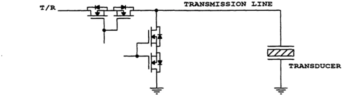
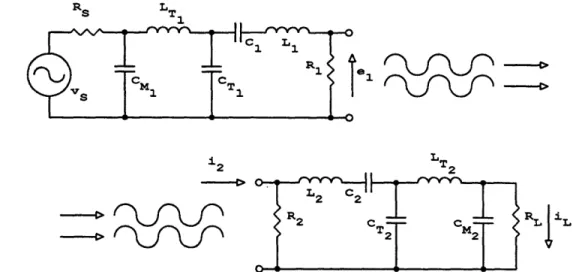
3.1 Equivalent Model of the BASS Transmit/Receive Process . . 3.2 Equivalent Model of the Transmit/Receive Process with the

M ultiplexer ... ... ... . 3.3 VN3205 N-Channel Enhancement Mode Vertical DMOS FET 3.4 Removing Capacitive Feedthrough Coupling with an FET

Shunt Switch ...

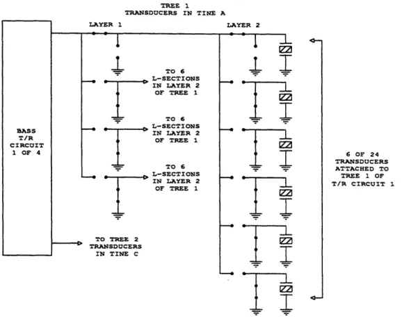
3.5 Quad FET L-Section ... ... 3.6 Two Layer Multiplexer ...

3.7 Schematic Diagram of the Completed L-Section ... 3.8 Address Structure for the MUX ...

3.9 Extended L-Section for P3 Operation ... . . ...

3.10 Equivalent Model of the Transmit/Receive Process with an Extended P3 L-Section ...

3.11 COSAC Schematic ...

3.12 Bessel Bandpass Filter Frequency Response - Magnitude .. 3.13 Bessel Bandpass Filter Frequency Response - Phase ...

S . . . . 82 . .. . . 83 S . . . . 86 S . . . . 88 89 S . . . . 96 S. . . . 106 . .... 110 ... . 113 ... 115 . .... 116 . .. .. 119 S. . . . 125 ... 127 S. . . . 136 ... 137 ... 144 . 148 ... 149

(18)

4.1 Definition Sketch for the Fresnel-Kirchoff Formula ... 154 4.2 Construction of the Ellipsoidal Sample Volume . ... 156 4.3 BASS Rake Acoustic Axis Geometry for the Fresnel Integral in a

Scattering Medium ... 165

4.4 Acoustic Axis Beam Width and Timing Window . ... 169

4.5 Acoustic Axis Beam Width and Timing Window Mapped

to the NIS . . . .... .... ... .... . . . .. .. .. .. ... 173 4.6 Real and Imaginary NIS Integrand Surfaces for a Logarithmic

Velocity Profile - Top View ... 178 4.7 Real and Imaginary NIS Integrand Surfaces for a Logarithmic

Velocity Profile - End View ... 179 4.8 Calculated Fresnel Zone Averages Along a Logarithmic Velocity

Profile - Linear Axes ... 180 4.9 Calculated Fresnel Zone Averages Along a Logarithmic Velocity

Profile - Semilog Axes ... 181 4.10 Real and Imaginary Parts of the Eikonal Normalized to Velocity

Space . . . .. . . . .. . . . 182 4.11 Real and Imaginary Parts of the Eikonal Normalized to Velocity

Space and Corrected for Systematic Bias . ... 183 4.12 Real and Imaginary Parts of the P2 Eikonal Normalized to Velocity

Space and Corrected for Systematic Bias . ... 185 4.13 Beam Pattern Approximations for a P2 Transducer Acoustic Axis . 188 4.14 Comparison of the Eikonal and Parametric Models of

Fresnel Zone Averaging ... 189 4.15 Beam Pattern Approximations for an Acoustic Axis Using

5MHz, 2.5 mm Transducers ... 192

4.16 Real and Imaginary Parts of the 5 MHz Eikonal Normalized to

Velocity Space and Corrected for Systematic Bias . ... 193 4.17 Further Comparison of the Eikonal and Parametric Models of

(19)

4.18 Imaging a Laminar Wave Boundary Layer with P2 Transducers . 196

4.19 Imaging a Laminar Wave Boundary Layer with 5 MHz, 2.5 mm

Transducers ... 197

4.20 Hypothetically Imaging a Laminar Wave Boundary Layer with P3 Transducers ... 198

4.21 Imaging a Turbulent Wave Boundary Layer with P2 Transducers. . 199 4.22 Imaging a Turbulent Wave Boundary Layer with 5 MHz, 2.5 mm Transducers ... ... 200

5.1 P2 Tine Showing Transducers ... 206

5.2 BASS Rake Laboratory Prototype . . . ... . . . . 207

5.3 Distortion of a Uniform Potential Flow by Two Round Tines . . . 209

5.4 Steady Flow Disturbed by Two Halfround Tines . . . . .... . . 211

5.5 WHOI Tow Tank and Carriage with the BASS Rake Laboratory Prototype ... ... 215

5.6 Surface Deformation During Tow Tank Calibration of the Laboratory Prototype ... ... ... 216

5.7 Measured Velocity During 30 cm -s- 1 _{Forward and Reverse Tows} _{. .} ₂₁₇

5.8 Gain Correction as a Function of Reynolds Number . . . 219

5.9 Single-Valued Mapping from umeas to ugc . .. .. . . ..... 221

5.10 Calibrated Measurement Accuracy of the Laboratory Prototype . . . 222

5.11 Calibrated Response in Oscillatory Flow at KC = 8 . . . 225

5.14 The 17 m Flume with the BASS Rake Prototype and LDV In Position . . . ... . . . .. ... . . . 230

5.15 BASS Rake Tines Positioned Over a Flat Sand Bed ... . . . 231

5.16 Along-Flume View of Laboratory Prototype and the Downstream Field of Bedforms ... .. 232

(20)

5.18 Bedform Field Under LDV Sample Volume ... 234

5.19 Velocity Records from the Zero Offsets Calibration . ... 235

5.20 Measurement of a 1 mm -s- 1 Current Driven by Thermal Convection ... 236

5.21 6 Minute BASS Rake and LDV Averages at Six Nominal Velocities . 237 5.22 BASS Rake and LDV Disagreement as a Function of Height for Each Trial . .... ... ... ... .. .... .. .. 238

5.23 BASS Rake and LDV Measurements of Turbulent Fluctuations . . .. 240

5.24 Bedform Propagation Past the BASS Rake Sample Volumes, Part 1 . 241 5.25 Bedform Propagation Past the BASS Rake Sample Volumes, Part 2 . 242 5.26 Flume Speed Fluctuations at a Nominal Velocity of 8 cm - s- 1 . ... 243

5.27 Detail from 8 cm -s- 1 Velocity Records . ... 244

6.1 The Assembled BASS Rake Field Prototype . ... 250

6.2 Zero Calibration of the Field Prototype ... . . . . . 251

6.3 Field Prototype Transducer Array . . . . 253

6.4 Definition Sketch for the Instrument Coordinate System ... . 255

6.5 Bottom Velocity Measurements in Great Harbor . ... 259

6.6 Spectra of the Velocity Measured 1 cmab . ... . ... 260

6.7 Velocity Profiles Over a Single Wave Cycle . ... 261

6.8 Gain Correction Surface as a Function of Tow Speed and Rotation A ngle . . . 265

6.9 Polar Presentation of the Gain Correction Surface . ... 266

6.10 Calibrated Measurement Accuracy of the Field Prototype ... . 268

6.11 Coastal Chart and Bathymetry for the Woods Hole Area ... 270

6.12 Coastal Chart and Bathymetry for Nobska Beach . ... 271

6.13 Anchor and Anchor Line Securing the Field Prototype to the Bottom . . . . .. . . . . .. . .. . ... . . . .. . . .. . . . . 272

6.14 Nobska Beach and the Deployment Area . ... 273

(21)

6.16 Sand Ripples Near the Tines . . . . .. .. . . . 275

6.17 Regular Sand Ripples at Site 2 . . . ... . . . . 277

6.18 Velocity Measurements at Level 3 for December 11, 1996 . . . 280

6.19 Running Averages of the Level 3 Velocity Components for December 11, 1996 ... 281

6.20 20 Minute Standard Deviations and Means for December 11, 1996 . . 282

6.21 20 Minute Standard Deviations and Means for December 7, 1996 . . . 283

6.22 Wave Spectra for December 7, 1996 . . . . 284

6.23 3 Minute Time Series, 1600 hours on December 7, 1996 . . . . .... . . 290

6.24 3 Minute Time Series, 1900 hours on December 7, 1996 . . . . 291

6.25 3 Minute Time Series, 2200 hours on December 7, 1996 . . . . 292

6.26 A Single Wave Cycle from the December 7 Storm . . . . 294

6.27 Velocity Profiles for the December 7 Storm Wave . . . . 295

6.28 A Single Wave Cycle from the December 7 Flood Tide . . . 296

6.29 Velocity Profiles for the December 7 Flood Tide Wave . . . 297

6.30 Wave Spectra for December 11, 1996 . ... 298

6.31 3 Minute Time Series, 1400 hours on December 11, 1996 . . . 299

6.32 3 Minute Time Series, 0445 hours on December 11, 1996 . . . 300

6.33 Velocity Profiles During the December 11 Ebb Tide . . . 301

6.34 Velocity Profiles During the December 11 Flood Tide . . . 302

A.1 Definition of Terms for the Governing Equations ... . . . 311

A.2 Velocity and Stress Profiles for a Laminar Wave Boundary Layer. . . 324

A.3 Magnitude and Phase of Velocity and Stress for a Laminar Wave Boundary Layer ... ... 325

A.4 Velocity and Stress Profiles for a Turbulent Wave Boundary Layer . . 327

A.5 Turbulent Stress Profiles Over an Extended Vertical Range . . . 328

A.6 Magnitude and Phase of Velocity and Stress for a Turbulent Wave Boundary Layer ... 329

(22)

B.1 Backplane ... ... 334 B.2 P2 {4, 6} Multiplexer Board ... 335

B.3 MUX Sequencer Board ... 336

B.4 Dummy Load ... 337

B.5 Tine Board ... 338

B.6 P3 {4,6} Multiplexer Board ... ... 339

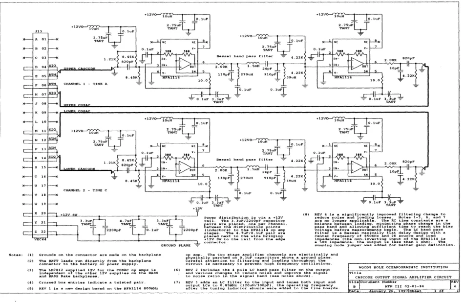
B.7 P3 Cascode Output Signal Amplifier Circuit (COSAC) . ... 340 B.8 BASS Transmit/Receive Board ... 341

(23)

List of Tables

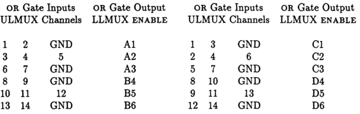
3.1 Allowed LLMUX Pairs ... 130 3.2 ULMUX Codes for LLMUX Pairs ... . 130 3.3 OR Gate I/O Assignments ... 130

5.1 Keulegan-Carpenter Numbers for Oscillatory Tow Cart Motions . . . 224

6.1 Gain Correction as a Function of Tow Speed and Rotation Angle. . . 264 6.2 Wave Boundary Layer Characteristics on December 7, 1996 ... 293

A.1 Wave Conditions for Laminar and Turbulent Wave Boundary

(24)

(25)

In a turbulent boundary layer, kinetic energy from the free-stream flow is converted into turbulent fluctuations and then dissipated into internal energy by viscous action. This process is continual, such that the turbulent

boundary layer is self-sustaining in the absence of strong stabilizing effects. For as long as these facts have been known, fluid dynamicists have sought to understand just how boundary-layer turbulence is generated at the expense of the mean motion, and just how it is dissipated. These are the objectives of studying the internal "structure" of turbulence. Since boundary-layer flows are the technical driver for so many engineering ap-plications, immense human and financial resources have been brought to bear on the problem over many decades of study. The progress made, however, has not been commensurate with the effort expended, reflecting the fundamental complexity of turbulence phenomena.

(26)

(27)

Chapter 1 Introduction

1.1 The Continental Shelf Wave Bottom

Boundary Layer

Conceptually, flow in the continental shelf bottom boundary layer can be decom-posed into mean and fluctuating components. It is common practice, in modeling the boundary layer, to solve the two cases separately and assemble the solution from the results. The mean flow is associated with tidal and other quasi-steady motions, with horizontal length scales from one to several tens of kilometers. Temporal scales are also large, typically no less than several hours and extending up to days and, occasionally, to longer periods. On the continental shelf, with depths no greater than 150 m to 200 m, the orbital velocities of wind driven surface waves penetrate to the bottom and give rise to the fluctuating component of the bottom boundary layer flow. The horizontal length scales of the oscillatory flow are only tens to hundreds of meters and temporal scales are only seconds to minutes. It is the wide difference in the temporal scales that permits the decomposition of the flow and that gives rise to the continental shelf wave bottom boundary layer.

The long time and horizontal length scales of the mean flow permit the current boundary layer to extend to the surface over the shelf unless the thickness is limited by stratification or Coriolis effects. In contrast, the short periods of wave motion

(28)

confine the wave bottom boundary layer (WBBL) to a thin sheet of sheared flow below an oscillatory, but essentially irrotational, core. The shear of the mean current remains important above the WBBL, but the oscillatory flow above the WBBL is well described by potential flow and linear wave theory. The vertical extent of the wave boundary layer is scaled by the period and strength of the near-bottom orbital velocity and by the interaction of this. flow with the mean current and the bottom. For a wide range of shelf conditions, the wave bottom boundary layer does not exceed 2.5 cm in thickness. Its depth is commonly no more than a centimeter.

The existence of the wave boundary layer has a number of important consequences. Because of the difference in vertical scale, the bottom shear stress associated with the wave flow can be up to an order of magnitude larger than the bottom stress caused by the mean current for comparable flow speeds. Even in relatively mild sea states, the wave induced bottom stress can be sufficient to initiate sediment motion. The wave boundary layer thus plays a central role in the entrainment of sediment into the water column. The strong shear in the narrow boundary layer increases the turbulent dissipation of flow energy so that the apparent roughness of the bottom, as seen by the mean flow, is much larger than would be expected for the scale of the physical roughness elements. The increased turbulence acts to keep entrained sediment in suspension. The mean current, which could not have entrained the sediment, then produces a net advective transport, potentially over the long horizontal scales of the steady flow.

Sediment transport is an area of active experimental and theoretical research. The movement of sediment in the nearshore environment has obvious links to coastal erosion, the maintenance of navigable harbors and channels, and the stability and longevity of shelf based structures. Accurate interpretation of the geological record on the shelf is dependent on knowledge of erosional and depositional processes. Equally important is the movement of contaminated sediments introduced by dumping or dredging operations. The resulting degradation of water quality is a public safety issue both for its effect on recreational use of the sea shore and its effect on commercial fisheries. Less obvious are the implications of down slope transport of sediment on

(29)

atmospheric CO2 levels. Briefly, the hypothesized removal of carbonaceous sediment from the bottom of the shelf based oceanic carbon cycle casts the ocean as a long term sink for carbon re-introduced into the global carbon cycle by the mining and burning of fossil fuels.

Our understanding of these processes is limited by the absence of any high resolu-tion field observaresolu-tions. Many laboratory studies have been conducted, but sediment beds in wave tanks and flumes have demonstrably different behavior than sediment beds on the shelf. Further, these studies were conducted with mechanically scanned, single measurement volume instruments and the measured vertical structure is neces-sarily an ensemble average over many wave periods. Stochastic stationarity is required over the period of measurement. It might be argued that this is sufficient for the mean flow or for monochromatic waves, the controlled conditions of the laboratory. How-ever, resolution of the vertical structure of the spectral waves typical of the shelf or of the vertical coherence of the turbulent fluctuations at the heart of boundary layer behavior is impossible. Critical aspects of boundary layer flow, in or out of the labo-ratory, are simply invisible to a sensor with a single measurement volume. Finally, it is difficult to combine waves and currents in the laboratory, particularly at the high crossing angles common on the inner shelf. Field studies of the WBBL have been rare and have been conducted with equipment that is not well suited to the task. In addi-tion to the deficiencies associated with single measurement volume instrumentaaddi-tion, the sensors used have been too sensitive to variations in environmental conditions and have lacked the mechanical robustness necessary for reliable, autonomous operation on the shelf.

Analytical, semi-empirical and numerical models of the wave-current boundary layer have been used to supplement and guide these studies. Field observations are required to establish or constrain the parameters of the models. For example, the hydrodynamic roughness, the roughness of the bottom as perceived by the flow, is a required input to most boundary layer models. Typically, this quantity is not modified as the model converges. The hydrodynamic roughness depends on grain size, bedform shape and scale, and sediment movement. The dependence is complex,

(30)

non-linear, and poorly characterized. No field measurements have made a spatially dense velocity profile through the WBBL from which the bottom roughness could be determined. Thus there is no well defined empirical relationship between the hy-drodynamic roughness and the physical bottom roughness, a quantity that could be measured directly, as the other initialization parameters are, and used to start the model. Like the laboratory experiments, the models often focus on fairly simple cases, with monochromatic, bi-directional waves, co-directional currents, and relatively sim-ple, non-erodable bottom geometries. Conditions on the shelf are significantly more complicated than those that can commonly be created in the laboratory or in a model. The wave field is neither monochromatic nor bi-directional in general, the angle of the current changes on several time scales and is often large, and the sediment is highly variable spatially and temporally over a range of characteristics.

Resolving the dynamic structure of the wave boundary layer requires a sensor with multiple sample volumes and fine vertical resolution. The sensor must be physically robust and the measurement must be insensitive to the wide range of environmental conditions found on the continental shelf, particularly the near-shore zone. Such an instrument would be able to image wave boundary layer flow, producing profiles from fully concurrent velocity measurements as well as averaged ensembles. Vertically coherent turbulent structures could be investigated and a better empirical relationship between the physical and the hydrodynamic roughness could be established. An instrument with multiple sample volumes could also directly measure the velocity immediately above the wave boundary layer, the forcing function of the linearized governing equation for boundary layer flow. A surrogate measurement of pressure, surface wave height, or the velocity well above the boundary layer could be avoided. This thesis documents the development, evaluation, and successful field deploy-ment of an instrudeploy-ment, the BASS Rake, specifically designed to support the require-ments outlined above. The BASS Rake uses the differential acoustic travel time technique of BASS, the Benthic Acoustic Stress Sensor, applied to a geometry suit-able for the narrow confines of the continental shelf wave bottom boundary layer. The instrument uses many sample volumes and the measurement technique has an

(31)

established record of accuracy and reliability on the continental margin. The BASS Rake makes it possible to profile a thin boundary layer, in the field, under essentially arbitrary conditions. The method and equipment are robust to fouling, sediment transport through the sample volume, and physical loading by the flow. Steady, monochromatic, and broadband spectral flows can all be meaningfully profiled. Sta-tionary conditions are not necessary. These abilities are currently unique to the BASS Rake.

1.2 Research Contributions

The success of this project rests on several technical innovations and intellectual contributions. Each plays an important role in the production of a functional and proven instrument from the elementary conceptual design. The first of these is the integrated mechanical design of the BASS Rake sensor head. Four tines support the acoustic transducers and the transmission lines in a geometry dictated by the nature and scale of flow in a wave boundary layer and by the use of the BASS differential travel time technique. The design balances the number and spacing of transducers available to image the flow against minimum wire diameters, electrical and acoustic cross-channel interference, flow disturbance by the sensor, ease of manufacture, and mechanical strength. To achieve that balance, most of the physical elements of the sensor head serve in several roles, often acting in the electrical design as well as the mechanical one.

The accuracy and stability of the BASS measurement depends critically on the electrical characteristics of the transmit/receive circuit and the transmission lines connecting that circuit to a pair of transducers. Full utilization of the BASS Rake transducer array requires a multiplexing interface between the transmit/receive circuit and the transducers. No commercially available interface approaches the character-istics and performance necessary to preserve the quality of the BASS measurement. The second contribution is a flexible interface with extremely low through resistance and an innovative structure that optimizes signal loading, provides significant noise

(32)

and cross-channel isolation, and preserves the electrical characteristics of the trans-mit/receive circuit and the transmission lines. It should be emphasized that the mechanical and electrical designs did not evolve independently. By intent, many fea-tures of each design address and solve the identified deficiencies of the other. The operation of the sensor depends on this integrated approach.

Characterizing and understanding the response of a sensor is critical to the devel-opment of any instrument. In the case of the BASS Rake, two processes affect the response. The first is velocity averaging over the Fresnel zone, the effective sample volume of an acoustic path. To understand and predict the effects of the averaging process, it was necessary to develop and solve a complex model describing acous-tic propagation in a scattering medium on the scale of a BASS Rake acousacous-tic axis. Because the proposed measurement required a close approach to the bottom, it was also necessary for the model to include the interaction of the sample volume and the boundary. It appears that this problem has not previously been solved for these conditions. The complex model was used to predict the circumstances under which Fresnel averaging would produced errors in velocity measurements and those results were confirmed empirically during flume and laboratory testing. A simpler parametric model of the averaging process was also developed and shown to produce substantially the same results with considerably reduced computational overhead. The faster para-metric model is now an important tool in the design of the BASS Rake transducer array.

The second, and far more significant process affecting the response of the BASS Rake, is the flow disturbance caused by the tines. The disturbance and the effect on the measurement were predicted, estimated, and bounded using a simple model. The Reynolds number and angular dependencies for both steady and oscillatory flow were determined in a tow tank, confirming the predictions of the model. The results and the explanation based on the model are consistent with the literature for flow around bluff bodies. This is the first time a Reynolds number dependence has been explicitly demonstrated and quantified for any BASS instrument. Once the effect had been determined, a mapping was developed from the measured velocity to the undisturbed

(33)

velocity and incorporated in the calibration and accuracy estimate of the instrument. The calibration was then verified in a flume over a sand bottom.

After laboratory evaluation was completed, a field prototype was constructed and deployed outside the surf zone of a local beach. Velocity profiles beginning within millimeters of the bottom were measured inside a 6 ms window at one second intervals for a period of several weeks. The instrument proved reliable, recording through several storms and revealing an asymmetric tidal dependence for both the waves and the mean flow. Regular reworking of the bed was observed and the velocity profiles showed clear evidence of the advection of turbulent eddies through the sample volumes. The data set is unique in that it contains concurrent velocity time series, of several weeks duration, with coverage from 1 cm to 20 cm above the bottom. The demonstrated reliability of the instrument and the return of a field data set were the final, important steps in the development of a functional and now proven instrument design.

1.3 Development Chronology and Thesis Outline

The possibility of applying the BASS differential travel time measurement to the wave bottom boundary layer was first raised in early 1993, but not pursued until the middle of 1994. At that time the integrated mechanical design of the sensor head began to evolve. A functioning prototype of that portion of the design underwent very preliminary tests in January of 1995. Those tests demonstrated that a BASS acoustic axis could operate in close proximity to a natural bottom, validating the most basic requirement of the proposed design.

The characteristics of the electrical interface required for full function of the trans-ducer array were specified in the spring of 1995. The constraints were too tight to be met by commercially available circuits and, over several months, specialty compo-nents with promising characteristics were identified and a design that could support the requirements was developed. Circuit cards, a chassis and backplane, new versions of the sensor head, and operating software were fabricated and written during the

(34)

fall. Most of these activities competed for time with a tight cruise and instrument rescue schedule. The laboratory prototype was assembled and ready for evaluation in January of 1996. Many difficulties, mostly related to the small transducers, were encountered and solved over the course of the spring. Once functional, the flow dis-tortion of the laboratory prototype was mapped in the tow tank. The evaluation of the Fresnel averaged sample volume was also undertaken at this time. Late in the summer these corrections were applied during a comprehensive set of flume tests. Working over a sand bottom, the operation and accuracy of the laboratory prototype were proven.

The BASS Rake field prototype was designed and built during the fall of 1996 and successfully deployed outside the surf zone of a local beach in both November and December. Twenty-four days of field data, velocity profiles recorded at 1 Hz, were extracted from the logger in January. Processing and analysis took place at various times over the winter. The data set shows regular reworking of the sand bed and the growth and evolution of ripples during storm and tide induced bedload transport is apparent. Tidal modulation of both the quasi-steady current and the waves on semi-diurnal, semi-diurnal, and spring/neap time scales is pronounced. The flow was shown to exhibit several asymmetries which could lead to the net advective transport of sediment.

The details associated with the events of this brief summary are documented in the chapters that follow. Chapter 2 focuses on the mechanical design of the BASS Rake. It begins with general background information about some of the major influences guiding the underlying design philosophy. The time and length scales of the wave boundary layer are detailed and the constraints these impose on the mechanical design are identified. The discussion of boundary layer scales is based on information that can be found in the literature. Some of the most important aspects of these studies

are summarized and discussed in Appendix A. The discussion in Chapter 2 then turns to models of the continental shelf boundary layer and a lengthy assessment of existing instrumentation. Finally, the mechanical design of the BASS Rake sensor

(35)

The electrical design, specifically the multiplexing interface between the trans-mit/receive circuit and the transducer array, is the subject of Chapter 3. The in-terface specification is presented through a discussion of the characteristics of the existing BASS circuitry and the mechanical design that provide the primary con-straints. The interface design is then laid out, beginning at the component level and proceeding to larger circuit blocks. The design includes both the signal path and the more conventional hardware, firmware, and software needed to control operation. A complete set of schematic diagrams is provided in Appendix B. The chapter con-cludes with a description of the modifications to the basic circuit that are required when measurements are made with particularly small piezoelectric transducers.

The sample volume of a single acoustic axis is determined in Chapter 4. The discussion begins with the classical theories of wave propagation and progresses to the more complex case of propagation through a scattering medium. A mathematical form, a Fresnel integral, describing a BASS differential travel time axis is derived and solved analytically for two canonical cases. A numerical solution for flow in a logarithmic boundary layer is presented and then used to assess a simple parametric model of the averaging process. The effects of Fresnel averaging in the continental shelf wave bottom boundary layer are determined using the parametric model. The simple model is also used to specify the necessary characteristics of the transducer

array for accurate imaging within a few millimeters of the bottom.

Chapter 5 documents the implementation and evaluation of the mechanical and electrical designs in the laboratory prototype. Details of the prototype's construction are presented, followed by a qualitative model of the flow distortion associated with the tines. The model accurately bounds the effects of the distortion on the measure-ment. Tow tank tests used to characterize the Reynolds number dependence of the response in steady flow and Keulegan-Carpenter number dependence in oscillatory flow are described. These results are incorporated in a non-linear sensor calibration mapping and applied to profile measurements made in a flume over a sand bottom. The calibrated measurements are presented and shown to match concurrent measure-ments made using a laser Doppler velocimeter to a high degree of precision.

(36)

The BASS Rake field prototype is described in Chapter 6. The important features of the support frame and the sensor are summarized and the results of a brief immer-sion in Great Harbor are presented. The tow tank calibration is then detailed. The response of the field prototype is more complex than that of the laboratory prototype because it depends on both the magnitude and the angle of the flow. A description of the near-shore field deployments at Nobska Beach, including visual observations of the bottom at both sites, follows. Selections from the returned field data, several weeks of 1 Hz velocity profiles, are analyzed and discussed at length to conclude the chapter. A general summary with suggestions for future development and research is presented in Chapter 7.

Finally, a few thoughts on the material selected for inclusion seem appropriate to close this chapter. Research is the work of detectives. It begins with a question. As the question is explored and knowledge deepens, it may be refined or changed. Different avenues appear and decisions are made to explore or postpone their inves-tigation. Some alleys are dead ends, yet they may return considerable information. It is only in hindsight and after reflection that the path behind may appear less ill defined and cluttered. The detective story often reaches a sense of closure, of un-derstanding, at the end. In science that closure is, happily, a transitory experience. A successful development raises new and deeper questions and provides an improved ability to address them. I have tried, in the chapters that follow, to describe not just the instrument that worked, but some of the more important developments and vari-ations that were tried along the way. It would be wrong to regard these as failures. Several will be indispensable to future versions of the BASS Rake. Throughout the development it has been the work done to understand and resolve the difficulties and setbacks that has reliably produced the greatest improvements in performance. This is the nature, and part of the pleasure, of research.

(37)

Chapter 2 Boundary Layer Scales and the

Mechanical Design of the Sensor

Headt

2.1 Introduction and Background

This chapter describes the development of the mechanical design of the BASS Rake sensor head. The characteristic scales of flow in the wave bottom boundary layer (WBBL) on the continental shelf and an evolving understanding of the capabilities of the BASS measurement technique have guided the design process. BASS Rake measurements are made using the BASS differential travel time (DTT) technique developed in and used by this laboratory [90]. This method was chosen because of its high accuracy and linearity and because of its extreme robustness to environmental conditions. These are necessary characteristics for any boundary layer instrument, particularly one intended for field use. The established electronic noise floor of the BASS measurement is 0.3mm - s- 1 _{[53, 90, 92]. Measurements are accurate to 1 %,}

inclusive of flow disturbance, and linear over the range ±240 cm - s- 1 [90, 92]. Flow disturbance is a more serious issue for the BASS Rake and will be discussed briefly in

t Some of the material presented in this chapter was originally published in Proceedings of the IEEE Fifth Working Conference on Current Measurement [55].

(38)

this chapter and at greater length in Chapters 5 and 6. Extensive field use has shown that BASS performance is not sensitive to the concentration of sediment in the water column. The measurement is influenced by biofouling, but only to the extent that marine growth may increase the flow disturbance. For example, the acoustic signal is not blocked by barnacles or seaweed attached to the transducer face, but flow noise may increase or the turbulent spectrum may change for smaller eddy scales. In one extreme case, the instrument continued to function while an octopus occupied the acoustic volume. Measured velocities were near zero. For storms, other high current and wave events, and use in or near the surf zone, failures are functions of the strength and stability of the support structure. Accurate measurements generally continue in these cases as long as power is maintained. However, rotation to a global Cartesian frame may be compromised by environmental modifications to the support structure. This has also been true of the occasional interaction with fishing trawlers [93].

A BASS DTT measurement is made by a pair of disk shaped, piezoelectric ceramic transducers, facing each other along an acoustic measurement axis. The differential arrival time of signals started simultaneously and traversing the axis in opposite directions is proportional to the average velocity along the axis [90]. The nominal relationship is

At = 2LU-, (2.1)

where t is time, -a~x, is the average along-axis fluid velocity and c is the local speed of sound, assumed to be constant over the path length, L. Equation 2.1 involves several simplifications which will be explored more fully in Chapter 4. The relationship, as given and assuming the accuracy of the simplifications, is correct to approximately 1 part in 106 for oceanic fluid velocities and a BASS sensor as commonly arranged and deployed. Transducer separation is normally 15 cm with a 10 ps signal pulse at 1.75 MHz. The 0.3mm m s- 1 single measurement accuracy is achieved by running each measurement with both forward and reversed receiver connections to remove bias. A single measurement cycle, inclusive of propagation and processing time, requires 320 ps. This allows a wide operational bandwidth and the use of multiple

(39)

sample volumes with nearly simultaneous measurements. For example, 100 acoustic axes forming an array could be polled inside a 35 ms window. The reader is referred to Williams, et al. [90] for additional information about the BASS DTT measurement. The primary focus of the mechanical design is the arrangement of these acoustic measurement axes. The geometry of the axes must be tailored to sample the velocity structure of the continental shelf WBBL. That structure is confined to a thin sheet of oscillatory shear flow overlying the sediment bed. For a broad range of shelf conditions, the vertical extent of the WBBL is less than 2.5 cm. A more detailed discussion of wave boundary layer structure can be found in Appendix A. Suitable references, listed in the bibliography, include Kajiura [38], Smith [73], Davies, Soulsby, and King [13], Grant and Madsen [24, 27] and Madsen [46]. This chapter assumes working familiarity with wave-current boundary layer flow and terminology on the part of the reader.

Imaging the velocity structure in such a narrow region requires very high vertical resolution. Observing the dynamic structure, particularly of wave flow during non-stationary conditions, requires multiple sample volumes. No existing field capable instruments meet these requirements. Detailed resolution is available in the labora-tory with some instruments or by constraining the flow to produce artificially thick wave boundary layers. However, most of these techniques employ only one sample volume. Profiles are built up over time by mechanically scanning across the boundary layer. This is legitimate in the laboratory where the flow can be controlled and con-ditions are relatively stationary, but those are not the concon-ditions found on the shelf. The inability to dynamically image boundary layer structure on the shelf, and often in the laboratory, limits further study and understanding of boundary layer processes and their effects.

Multiple sample volumes, spanning the WBBL and also sensing the irrotational oscillatory core immediately above it, have the added advantage of providing a direct, correlated measurement of u,, the forcing input to the linearized governing equation for the boundary layer.

du

du,

_87lp

-9u a= t + -rp (A.21)

(40)

The derivation and solution of Equation A.21 are the subjects of Appendix A. A direct measurement would also contribute to greater understanding of boundary layer structure and behavior. Previous measurements have used indirect measures as sur-rogates for the forcing term. One common practice has been to measure pressure, generally well above the boundary layer. Alternatively, u. has been determined by applying linear wave theory to surface wave measurements or to velocity measure-ments. In either case the measurement is made well above the boundary layer.

For the BASS Rake, resolution depends on both the geometry of the acoustic axes and on the resolution of an individual axis. Consideration of the individual sample volume and its effects on the response of an acoustic axis will be postponed until Chapter 4. This is a complex process that has not previously been examined in detail for a BASS sensor. Here it is noted that the extent of the sample volume is largely determined by the acoustic frequency. A conscious decision was made early in this development not to treat the acoustic frequency as a design parameter. This was done for two reasons. First, it was recognized that significant changes to an already tightly constrained transmit/receive (T/R) circuit would be necessary to support the large number of channels and the flexible acoustic axis selection of the proposed BASS Rake transducer array. These changes are the subject of Chapter 3. Other components currently used in BASS have effective operational bandwidth limits less than an order of magnitude above the signal frequency. It. was therefore desirable to avoid any additional changes to the underlying BASS circuitry made necessary by large changes in the operating frequency.

Second, the piezoelectric transducers are driven at their resonant frequency. This is fixed during production because it depends on the material properties and physical dimensions of the disk. Therefore, any change in operating frequency requires new transducers. Neither the production delay nor the financial cost are inconsequential. These concerns were particularly cogent during the time and budget limited proto-typing phase of the BASS Rake development documented by this thesis. There are, however, potential benefits to a change in frequency that, because of this work, can now be understood and predicted with some confidence. These are explored with a

(41)

parametric model in Chapter 4. There it will be shown that a relatively small increase in the frequency of the acoustic signal can significantly improve vertical resolution. Changes to the operating frequency will be undertaken in the future as part of the continuing development of the Rake.

In consequence, the mechanical design discussed in this chapter tries to optimize resolution as a function of the axes geometry defined by the transducer array. The diameter and spacing of the transducers are the primary design variables. Constraints are provided by the magnitude of the flow disturbance caused by the transducers and the structure supporting the array. The electronics, particularly the transducer sig-nal lines, impose a number of constraints that require mechanical as well as electrical solutions. For example, the volume of the transducer wiring harness must be mini-mized without sacrificing environmental and cross-channel signal isolation. Dynamic flexure of the lines must be eliminated to preserve the zero offset calibration [53]. Ohmic transmission line terminations must be made to both faces of each transducer, yet the T/R face should remain unobstructed to maintain a clean beam pattern and to reduce transmission loss. Mechanical alignment of the transducers and stiffness of the structure should be assured by the design. Issues related to the ease and cost of manufacture should not be ignored. These examples do not constitute an exhaus-tive list. All of the design variables and constraints are interrelated and each change requires trade-offs to maintain a balanced design.

One of the principal contributions of this research is the integrated design of the support structure and transducer mounting. The transducer support tines of the BASS Rake, which will be described in Section 2.4, successfully addressed the design requirements, resolving many of the conflicting imperatives. The remaining problems were solved by integrating the development of the new electronic interface (Chapter 3) into the overall design process. The success of the design depends on balanced trade-offs between resolution and flow disturbance and on innovations which eliminate many of the electro-mechanical difficulties. The result is a high resolution, multiple sample volume instrument that is robust to field conditions.

(42)

in-fluencing the design of the BASS Rake. The characteristic scales of the continental shelf WBBL, which this new instrument is tailored to sample, are discussed in Sec-tion 2.2. More detailed informaSec-tion about the structure of the wave boundary layer can be found in Appendix A and in several of the references [45, 46, 80, 81]. The motivation to design and construct this instrument arose from the inability to make accurate, detailed structural measurements of the continental shelf WBBL with ex-isting instrumentation. Previous laboratory and field studies have used a variety of techniques to make near-bottom velocity measurements. Section 2.3 examines several of these investigations with regard to the strengths and the limitations of the instru-ments used, and their suitability for dynamic profiling in the field. The design of the BASS Rake specifically targets several of those limitations. The design of the sensor head is presented in Section 2.4. That section also includes a preliminary analysis of measurement errors caused by flow distortion. Comparisons between the various techniques are made throughout the chapter with a short summary of the principal strengths and weaknesses of the BASS Rake presented in Section 2.5.

2.2 Characteristic Scales of the WBBL

Resolving the dynamic structure of the wave bottom boundary layer, as with any process, requires accurate measurements with spatial and temporal spacings that are small compared with the characteristic scales of flow in the layer. A reasonable working target is measurement granularity an order of magnitude smaller than the flow scales to be resolved. It should be recognized, however, that this level of detail may not be possible or that it may be insufficient to prevent aliasing of still smaller features. Flexibility and caution are required in applying any design rule.

Several of the characteristic scales of the WBBL have been estimated here based on the Grant and Madsen (GM) wave-current boundary layer model [24, 27, 45, 46]. [24] and [27] describe early versions of the model. The most recent and complete definitions are found in [45] and [46]. Some features of the GM model are discussed in Section 2.3.1. Additional details can be found in Appendix A. Nominal values