A comparative study of geometric transformation models for the historical "map of france" registration

HAL Id: hal-01416127

https://hal.archives-ouvertes.fr/hal-01416127

HAL is a multi-disciplinary open access archive for the deposit and dissemination of sci-entific research documents, whether they are pub-lished or not. The documents may come from teaching and research institutions in France or abroad, or from public or private research centers.

L’archive ouverte pluridisciplinaire HAL, est destinée au dépôt et à la diffusion de documents scientifiques de niveau recherche, publiés ou non, émanant des établissements d’enseignement et de recherche français ou étrangers, des laboratoires publics ou privés.

A comparative study of geometric transformation

models for the historical ”map of france” registration

Pierre Alexis Herrault, David Sheeren, Mathieu Fauvel, Claude Monteil,

Martin Paegelow

To cite this version:

Pierre Alexis Herrault, David Sheeren, Mathieu Fauvel, Claude Monteil, Martin Paegelow. A com-parative study of geometric transformation models for the historical ”map of france” registration. Geographia Technica, Cluj University Press, 2013, pp. 34-46. �hal-01416127�

To cite this version : Herrault, Pierre Alexis and Sheeren, David and Fauvel, Mathieu and Monteil, Claude and Paegelow, Martin A comparative study of geometric transformation models for the historical "map of france" registration. (2013) Geographia Technica (n° 1). pp. 34-46. ISSN 1842-5135

Open Archive TOULOUSE Archive Ouverte (OATAO)

This is an author-deposited version published in : http://oatao.univ-toulouse.fr/ Eprints ID : 16318

To link to this article :

URL : http://technicalgeography.org/index.php/latest-issue-1-2013/71-05_pierre-alexis_herrault_david_sheeren_mathieu_fauvel_claude

Any correspondence concerning this service should be sent to the repository administrator: staff-oatao@listes-diff.inp-toulouse.fr

A COMPARATIVE STUDY OF GEOMETRIC TRANSFORMATION

MODELS FOR THE HISTORICAL

‘MAP OF FRANCE’ REGISTRATION

Pierre-Alexis Herrault1, 2_{, David Sheeren}1_{, Mathieu Fauvel}1_,

Claude Monteil1, Martin Paegelow2

Abstract

It is widely recognized that present-day biological diversity may reflect past land use and landscape features. Understanding the historical background is essential to explain the ecosystem functioning of landscapes today. Numerous historical spatial data have been used to reconstruct these pathways but resulted in problems of sources, formats and supports. One major problem is how to incorporate historical data in current coordinate systems to enable them to be compared with each other and with current sources. Previous works on the registration of historical maps already demonstrated the superiority of local methods (e.g. a Delaunay-based method) over global methods (like polynomial mapping models) because of the existence of local geometric distortions. The same studies also highlighted the importance of selecting ground control points with a homogeneous spatial distribution to improve the accuracy of registration. Furthermore, while kernel-based methods have already proved their efficiency for many other applications, they have rarely been used for map registration even though they provide an interesting alternative to conventional methods. In this paper, we present a comparative study of various geometric transformation methods to register an excerpt of the historical ‘Map of France’ (an Ordnance Survey map) dating from the 19th century. We compare the performance of several global and local methods with kernel-based methods (Gaussian and polynomials) and analyze the impact of the number of control points, their nature and their spatial distribution on the quality of registration. A protocol was developed to apply the transformation models in various situations and to identify the best strategy for the georeferencing of historical maps.

Key Words: Historical map registration, geometric correction, kernel regression. INTRODUCTION

It is widely recognized that present day biodiversity may reflect past land use because of a possible delay between changes in a landscape and changes in the associated plant or animal population. Knowing the historical background of landscapes is therefore a precondition to understanding ecosystems functioning (Jackson, 2006). Historical ecology concerns all the elements in a landscape. For example, using archival and archeological data (Hewlett, 1977), reconstructed river valleys in Great Britain from the year 1000. Later, other authors used similar approaches to explain current forest biodiversity with respect to forest history (Hermy and Stieperaere, 1981).

Different problems arise when users want to use historical spatial data, for instance maps drawn in the 19th century. Firstly, the variety of sources with different formats and supports increase the heterogeneity of spatial data. Secondly, because of the technical and financial means at that time, the quality of historical data may differ from one source to another and may lead to inconsistencies and biases in the assessment of landscape changes (Pontius and Lippit, 2006). Finally, these data are generally not georeferenced. In order to 1

University of Toulouse, INP-ENSAT, UMR 1201 DYNAFOR, Auzeville Tolosane, France. 2

incorporate them in current coordinate systems and to compare them with present data, a registration step (or georeferencing) is required. Georeferencing is a crucial step in the use of historical data. Several studies have already focused on this issue (e.g. Baiocchi and

Lelo, 2005; Bitelli et al., 2009).

Generally speaking, two main approaches are used for map (or image) registration: global or local (Zitova and Flusser, 2003).The global approach is appropriate when map distortions are homogeneous. With this method, only one transformation model is computed and applied using all available ground control points (GCPs). However, a local approach is more efficient if local distortions have to be taken into account. With this method, the map or image is partitioned into a set of regions and one transformation model is computed for each region individually.

The local approach is known to be more efficient to register historical maps (Fuse et

al., 2009). The low quality of the survey instruments, the lack of cartographical

specifications and the diversity of the surveying engineers and campaigns led to numerous local planimetric errors that cannot be handled correctly by global transformation models. However, other registration techniques could be used to improve the accuracy of the geometric transformation models. In particular, nonparametric methods like kernel smoothing regression are a possible alternative to conventional approaches because they are locally sensitive but provide one global model. These methods have already proven to be very efficient for many applications including image processing and pattern recognition (Shawe-Taylor and Cristanini, 2004; Takeda et al., 2007).

Like the number of points, the spatial distribution of the GCPs is also important in the map registration process since it may affect the accuracy of the transformation models (Mather, 1995; Wang et al., 2012). Regular spatial distribution of GCPs provides a best-fitting process but requires many points for efficient registration (Boutoura and Livieratos,

2006). In the case of old topographic maps, the GCP problem is often difficult to overcome

due to the possible change in the landscape objects over the past centuries and in the characteristics of the GCPs themselves (reliability and accuracy, kind of object, graphic representation). In contrast to aerial and satellite images, the effect of the sampling design of the GCPs, their number and their category on the geometric correction of old maps have been less studied.

The aims of this paper are to test and assess the potential of the kernel regression method to register an historical map from the 19th century. We compare the method with other global and local conventional approaches. Second, we independently investigate the effect of three parameters used to select GCPs on the accuracy of map registration:

1. The spatial distribution of the GCPs (regular or random); 2. The number of GCPs;

3. Whether the GCPs are reliable or unreliable.

The paper is organized as follows. In section 2, we describe the data and the experimental protocol with the kernel regression and other registration methods. In section 3 we present and discuss the results of the experiments. Finally, some conclusions are drawn along with some perspectives.

2. MATERIAL AND METHODS 2.1. Data

In this comparative study, we used an excerpt of the historical ‘Map of France’ produced from 1825 to 1866 at 1:40000 in the projection of Bonne. This excerpt covers an area of 20 km² in southwestern France surrounded by contrasting landscapes: valleys bottoms, mountains and a plateau. This historical Map of France is known for its planimetric accuracy, considerably better than the previous Cassini map published during the reign of Louis XV. Moreover, the Map of France is in color, which makes it easier for users to capture the cartographic elements. Last, the Map of France was produced in an interesting period for the study of the forest evolution. The extent of French forests was lowest around 1830 and then expanded continuously until today (Mather et al., 1999). Thus, if an existing forest appears on the old map, it might be unchanged for several decades.

Fig. 1. Excerpt of the Historical 'Map of France' used in this study with examples of forest features.

The GCPs were selected from an existing database of aerial photographs: the BDOrtho® produced by the French National Mapping Agency (IGN). The image has a spatial resolution of 0.50 m.

2.2. Methodology

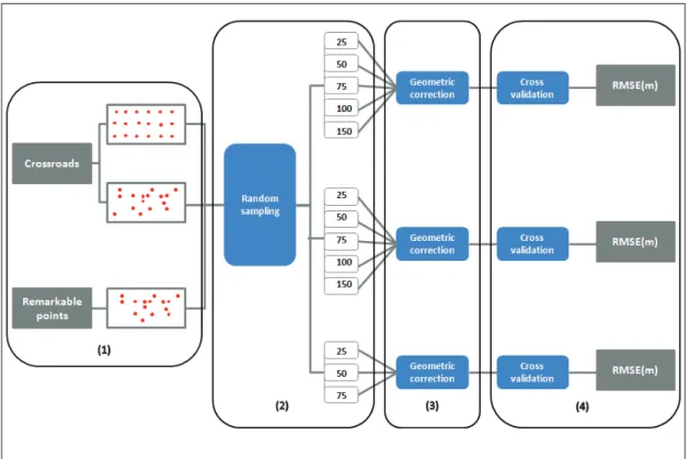
An experimental protocol was defined (Fig. 2) to compare the registration methods. The protocol comprises four main steps: (1) acquisition of a high number of two categories of control points in the old and reference maps according to two spatial distributions (random and regular), (2) creation of GCP subsets of various sizes, (3) computation of several transformation models, (4) validation and comparison of the results.

Fig. 2. Experimental protocol applied to evaluate the effects of the nature, the number and the spatial

distribution of GCPs on the registration accuracy.

In the first step (1), we identified landmarks and crossroads to assess the impact of the categories of GCP on the accuracy of the geometric transformations. We assumed that the landmarks are more accurate than the crossroads. Indeed, these points (chapels, churches, mills, etc.) were used as reference points when topographical surveys were being conducted before the map was drawn. For this reason, their absolute planimetric accuracy might be higher than other points on the map, particularly the crossroads.

A total of 75 randomly distributed landmarks were found on the old map. For the crossroads, we selected 150 GCPs according to two spatial sampling processes: random and regular. The regular distribution was obtained from a regular grid covering practically the entire map and divided into 12 x 20 squares. For the landmarks; we only used random distribution because the small number of points prevented regular sampling.

In the next step (2), we created GCP subsets with the aim of assessing the impact of the number of points on the accuracy of the transformation models. The number of points in these sets ranged from 25 to 150 for the crossroads and from 25 to 75 for the landmarks.

In step (3), we compared the performance of several geometric transformation models for each configuration of the GCPs. Global and local methods were tested and compared to the alternative kernel regression approach. The methods tested are listed in

Table no. 1.

Table no. 1. The geometric transformation models compared.

Global Method locally non sensitive Global Method locally sensitive Local Method

Affine

Second order polynomial Third order polynomial

Linear Kernel

Second order polynomial kernel Third polynomial kernel

Gaussian kernel

• Conventional global and local registration methods

As mentioned above, previous works on the registration of historical maps have showed the advantage of local methods (like the triangle-based method) over global methods (polynomial mapping functions) because of the existence of local geometric distortions (White and Griffin, 1985; Fuse et al., 1998).

A global transformation simply means that all the control points are used to derive a single mathematical model of the geometric distortions. First order, quadratic or cubic models are the most widely used to register an image or a map. The general expression of the 2D polynomial model is defined as follows:

1 0 0 N N i j ij i j

x

a u v

"

##

y

b u v

"

##

where aij and bij are the coefficients of the equations ! = "(#, $) and % = &(#, $), the

reference coordinates being (#, $).

The degree of the polynomial model is defined by '. For ' = 2, the polynomial function can be expressed as follows:

2 2 00 01 02 11 10 20

x

"

a

$

a v

$

a v

$

a uv

$

a u

$

a v

y

"

b

$

b v b v

$

$

b uv b u

$

$

b v

A minimum of three points (6 parameters) or six points (12 parameters) are needed to estimate the coefficients of the first order model (linear transformation) and second order model (nonlinear transformation) respectively. However, the number of equations is usually higher than the number of unknowns (i.e. there are more GCPs than the minimum number required). The coefficients of the mapping functions are then computed using least square fit, which provides residuals for each point.

In the case of the local transformation approach, after dividing the map into a set of regions, several local mapping functions are computed (Goshtasby, 1986, 1987). In general, the regions are created from a Delaunay triangulation and one first order polynomial function is computed per triangle. Each triangle is based on three GCPs and define a mapping function that is only valid within this region. According to (Balletti, 2006), the smaller the triangular areas of the mesh, the better the results. Thus, for this approach, it is important to collect a large number of control points to reduce the extent of the triangle.

• Kernel-based method

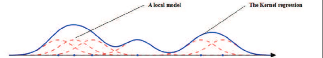
In this paper, we compare the performances of several global and local methods with kernel-based methods (Table no. 1). These models belong to the category of global methods but are able to take local distortions into account by combining local models computed in a bandwidth (locally weighted regression smoother, Fig. 3).

Fig. 3. Local models successive (red lines) and the global kernel regression (blue line).

(from (Takeda et al., 2007))

The previous conventional methods were compared with the kernel regression (Shawe-Taylor and Cristanini, 2004). Kernel regression is a non-parametric statistical technique that belongs to the category of global methods but which is locally sensitive since it enables local distortions to be taken into account by combining local models computed in a given bandwidth (locally weighted regression smoother). This method is efficient for the estimation of nonlinear relationships between variables with minimal assumptions about the model. The general expression of the model is given by the decision function (given here for the 1-D case for the sake of simplicity):

"(() = ) *+,(!+,() + -.

+/0

where ,(. . , . . ) is the kernel, *₊ the amplitude coefficients, - the bias, !₊ the learning samples and z, the predictive sample. The *₊ and - are the parameters to optimize. They are determined by minimizing the mean square error (MSE), i.e.:

123₄

5,6 )(%+7 "(!+))

8 _+9::"::8 .

+/0

where the 9 parameter is a regularization parameter that is used to prevent from overfitting.

After straightforward computations, the solution is given by (in matrix form):

;*<

-=> = %(?@+9A.B0)C0

where (%)+ =%+, (?@)_+,D =,(!+,!_D),(?_@)_.B0,D = (?_@)_+,.B0 = 1, (?@)_.B0,.B0= 0 and

The kernel is a positive semi-definite function. It is used to map the sample implicitly in a feature space where the relation between X and Y is easier to estimate.

In this paper, two kernels were investigated:

- Polynomial kernel: ?_E =FG!+,!DH + 1IE - Gaussian kernel: ?_J(!, %) = exp K7LMCNLO

8JO P

In the final step of the protocol (step 4), the results were validated and compared to identify the best registration approach. We used cross validation to assess the accuracy of each transformation process and in particular, the leave-one-out method. Cross validation is commonly used to estimate the accuracy of a predictive model. It involves dividing the observations into two subsets: one subset is used to train the predictive model and the other to validate it. This process is repeated several times to increase the reliability of the validation.

In the leave-one-out cross-validation, only a single observation is selected for validation and all the remaining observations are used as training data. This process is repeated such that each observation in the sample is used once as the validation data. The validation results are then averaged to compute an average error. In our case, the error index used for assessing the quality of the registration was the root mean square error (RMSE). Thus, after the cross-validation process, we obtained an average value of the RMSE (called RMSEm).

3. RESULTS AND DISCUSSION

We successively analyzed each parameter of the registration process in order to identify the best strategy for georeferencing the historical ‘Map of France’.

• Impact of the number of GCPs

This parameter was only assessed for the crossroads, of which there were many examples. Table no. 2 summarizes the results of different geometric transformation models using the five GCP subsets composed of 25, 50, 75, 100 and 150 points. The influence of the number of points was analyzed for the two spatial distributions available: random and regular.

Overall, the results showed that the number of errors decreased with an increase in the number of points regardless of the spatial distribution. For instance, we observed that, for the affine transformation, the RMSEm decreased by approximately 27 m from the GCP subset of 25 points to the subset of 150 points. The same was true for the kernel transformation. Using the Gaussian kernel, the average error decreased by 26 m (in the case of regular distribution) and by 37 m (in the case of random distribution) using a number of GCPs that ranged from 25 to 150. The Delaunay-based transformation was more sensitive to the number of points. The RMSEm followed the same negative trend but the initial number of errors was much higher than with the other transformation models. When the number of the GCPs is small, the size of the triangles is very large. Consequently, the local first order polynomial models are less accurate.

Table no. 2. RMSE(m) obtained by the different transformation models tested for 25 to 150 GCPs and for a regular or a random distribution of these GCPs.

• Impact of the spatial distribution of GCPs

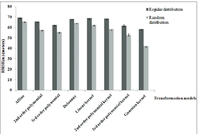
Concerning spatial distribution, Table no. 1 shows that the regular distribution is generally more efficient than the random one up to a set comprising 75 GCPs. While the error for the affine transformation varied between 131 and 88 ms for a random sampling, the average error ranged from 106 to 6 meters when the spatial distribution was regular. This is also true for the first and second order polynomial kernels. However, with over 75 GCPs, the trend was reversed in favor of random distribution (Fig. 4). The most accurate models are computed from a random sampling when large GCP datasets are used. In the case of the Gaussian kernel, the random distribution is always better.

Fig. 4. Comparison of the performance of registration methods for 150 GCPs and for a random or a

• Impact of the geometric transformation models

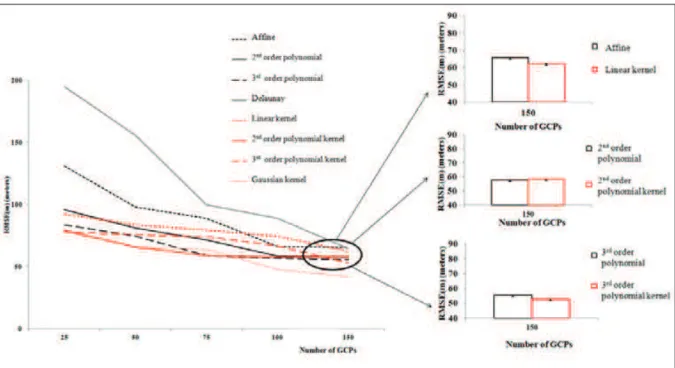
The performances of the geometric transformation models were only compared for the random distribution (Fig. 5).

Generally speaking, our results show that the differences in accuracy between the models are greater with small sets of control points than with large sets. When only 25 points were used, the best model was given by the Gaussian kernel (RMSEm equals 75 m). The least efficient model was the Delaunay-based transformation (RMSEm equals 195 m). As mentioned above, this local approach appears to be very sensitive to the number of points.

The results of the Gaussian kernel model were always better than the results of the other methods (except for the set of 75 GCPs). The Gaussian kernel model appears to be very efficient when the number of GCP is high (RMSEm equals 42 m for 150 GCPs). The third order polynomial kernel also gave good results with large datasets with an average error equal to 52 meters for 150 GCPs, up to 10 meters more than the Gaussian kernel transformation. Kernel-based methods are generally more efficient than conventional global models for equivalent transformation (see Fig. 5). This was the case for almost all the GCP sets (except for the set of 100 GCPs).

Fig. 5. Comparison of the performance of registration methods for 25 to 150 GCPs and for only one

random distribution of these GCPs - Focus on the comparison between conventional and kernel registration methods.

• Impact of the GCP categories

Finally, we assumed that landmarks (or remarkable points) are more accurate and provide better results.

Globally, this assumption was confirmed. In the majority of the cases, the RMSEm is lower when landmarks are used in geometric transformation models.

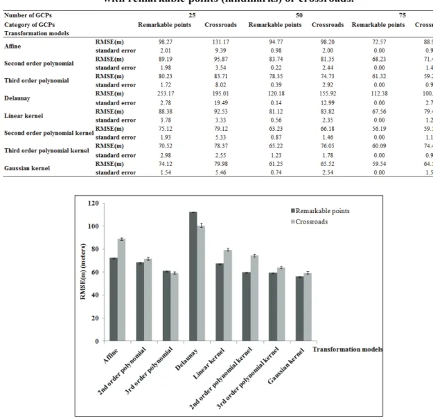
With the affine transformation the difference in errors between landmarks and crossroads ranged from 33 to 16 meters. The same relation was found for second order polynomial transformation and for kernel based transformations in general. For example, while Gaussian kernel transformation presents an average error of 64.12 meters with crossing roads (set of 75 GCPs), the mean of positional error was about 59 meters with landmarks for the same number of GCPs.

The trend was different with the second order polynomial and with the Delaunay-based transformation.

With the second order polynomial model, there was a slight difference in the number of errors using landmarks and crossroads, but overall, crossroads produced better results. The difference ranged from 2 to 4 meters. This opposing trend can be explained by the random sampling process. This step was performed using a GCP with 200 crossroads but only 75 landmarks. Furthermore, the standard error of the order three polynomial model using crossroads was much higher than that using landmarks so the variability of the results was not the same, hence explaining these contradictions.

Table no. 3. RMSE(m) obtained by the different transformation models tested for 25 to 75 GCPs with remarkable points (landmarks) or crossroads.

Fig. 6. Comparison of the performance of registration methods for 75 GCPs

As regards the Delaunay-based transformation, as we mentioned above, this model is very sensitive to the number of points. This time, the random sampling process using the crossroads category led to better spatial distribution. The probable explanation is that the size of the triangle was more regular in a few samplings, thus avoiding abrupt bias faults in some parts of the map.

Fig. 6 compares the transformations between the crossroads and the landmarks for

75 GCPs. Except for the Delaunay transformation and the third order polynomial, the landmark sets gave better results.

• Comparative analysis

The comparison of different geometric transformation models and the evaluation of some parameters in the selection of GCPs led to various teachings in order to find the best strategy.

First, the higher the number of GCPs, the lower the average number of errors. This is to be expected when predictive models are used for image registration: the higher the number of points used, the more local distortions are taken into account, and the more efficient the transformation will be. Moreover, the larger the sample, the lower the approximation so the model predictions are better and provide a good estimation of the transformation. Concerning this parameter, Delaunay triangulation appears to be a special case. Indeed, an increase in the number of GCPs leads to a spectacular decrease in the RMSE(m). This can be explained by the reduction in the size of the triangle that consequently takes local distortions better into account. With the other transformation models, the decrease in the number of errors between each GCP set was lower because the map registration is homogeneous and accomplished using all the GCPs.

The evaluation of spatial distribution revealed two major trends. When the number of GCPs is small, regular distribution is required. The explanation may be that regular distribution ensures global coverage of the region of interest. Even if the number is small, each part of the map is taken into account by the models, thus avoiding abrupt bias fault. A random distribution could lead to parts in the map being neglected and for that reason, not provide an accuracy transformation in all cases.

However, when the number of GCPs is high, random distribution is more efficient. Planimetric accuracy is not homogeneous in historical maps. Thus, local distortions can be solved by random distribution because the GCPs are not spatially constrained. Based on random sampling, random distribution appears to be more efficient for the registration of historical maps.

Next, we compared some global and local models and tested the potential of kernel based methods.

Overall, kernel based methods proved to be more efficient than conventional methods. When we focused on transformations with GCP sets numbering 150, the results of polynomial kernels were better than those of conventional polynomial methods, except for second order polynomials, whose results were very close.

The results of the Gaussian kernel method were the best. With 150 crossroads and random distribution, the average positional error was about 42 meters. This error is clearly lower than other transformations meaning that this method is a very accurate registration model and a very good alternative to methods currently employed in georeferencing of historical maps.

Finally, we analyzed categories of points. Distinguishing between landmarks and crossroads, we assumed that some points on the early map are reliable and others unreliable.

The results indicated that models using landmarks provided better transformations than the others. This result confirms that survey points are recommended in the creation of a GCP set. Nevertheless, their limited number (only 77 in this excerpt) meant we could not only use this category. Combining landmarks with crossroads was required to create GCP sets and to improve the transformations.

4. CONCLUSION

From this study, it appears that georeferencing of old maps depends not only on the transformation model used but also on the spatial distribution, the number, and the category of ground control points.

Kernel based methods proved to be more efficient than conventional methods. The comparison with currently used methods showed that kernel models enable early maps to be georeferenced most accurately. In particularly, the Gaussian kernel provided the best transformation.

Analysis of the spatial distribution of GCP, their number and their category, highlighted an optimal configuration for georeferencing. Indeed, random distribution is required to better account for local distortions in the historical map. In addition, the models are more efficient with a large number of points for two major reasons: the region of interest is more comprehensively covered and error estimation by the prediction models is better. Finally, the analysis of the categories of GCPs showed that landmarks are more accurate than crossroads, but that their number is not sufficient for optimal transformation.

This research could be extended to cover the following points:

First, the evaluation of Delaunay transformation showed that it was very sensitive to the number of GCPs. With 150 GCPs, it was less efficient than kernel based methods. However, with a large number of GCPs, it was more accurate than the other models tested . Combining landmarks and crossroads could thus greatly improve the results. Also, other categories of points could be analyzed to find the best combination of GCPs. Finally, we believe it is important to work on visualization of the error of transformation. This information could advance our understanding of local distortions to improve the local calibration of transformation models.

Acknowledgments:

This research was supported by the French National Research Agency (ANR JCJC MODE-RESPYR 2010 1804 01 – 01). P.-A. Herrault is also funded through a PRES Toulouse University and Region Midi-Pyrenees grant.

R E F E R E N C E S

Baiocchi V., Lelo K., (2005). Géoréférencement des plans historiques (du XVIIIe au XIXe) de la ville de Rome, et leur comparaison avec des cartes actuelles, Géomatique Expert 45, p. 42-47 Balletti C., (2006). Georeference in the analysis of the geometry content of early maps”,

Bitelli G., Cremonini S., Gatta G., (2009). Ancient map comparisons and georeferencing techniques : a case study from the Po River Delta (Italy), E-perimetron, 4-4, p. 221-233

Boutoura C., Livieratos E., (2006). Some fundamentals for the study of the geometry of early maps by comparative methods, E-Perimetron, 1-1: 60-70

Fuse T., Shimizu E., Morichi S., (1998). A study on geometric correction of historical maps, International Archives of Photogrammetry and Remote Sensing, 32(5), p.543-548.

Fuse T., Shimizu E., (2009). Vizualizing the landscape of old time Tokyo (Edo City), Commission V, WG V/6.

Goshtasby A., (1986). Piecewise linear mapping functions for image registration, Pattern Recognition, vol. 9, no.6, p. 459-466.

Goshtasby A., (1987). Piecewise cubic mapping functions for image registration, Pattern Recognition, vol. 20, no. 5, p. 525-533.

Hermy M., Stieperaere H., (1981). An indirect gradient analysis of the ecological relationships between ancient and recent riverine woodlands to the south of Bruges (Flanders, Belgium), Vegetation 44, p. 43-49.

Jackson S.T., (2006). Vegetation, environment, and time: The origination and termination of ecosystems, Journal of Vegetation Science, 17, p. 549-557.

Mather P.M., (1995). Map-image registration accuracy using least-squares polynomials. International Journal of Geographical Information Science, 9, pp. 543–554.

Mather AS., Fairbairn J., Needle CL., (1999). The course and drivers of the forest transition: The case of France, J Rural Studies 15, pp. 65–90.

Pontius GR., Lippitt CD., (2006). Can error explain map differences over time? Cartogr Geogr Inf Sci, 33, p. 159–171.

Shawe-Taylor J., Cristianini N., (2004). Kernel Methods for Pattern Analysis, - Cambridge University Press.

Takeda H., Farsiu S., Milanfar P., (2007). Kernel regression for image processing and reconstruction, IEEE Transactions on image processing, Vol.16, No.2, p 349-366.

Wang, J., Ge Y., Heuvelink G., Zhou C., Brus D., (2012). Effect of the sampling design of groundcontrolpoints on the geometriccorrection of remotely sensed imagery, International Journal of Applied Earth Observation and Geoinformation, 18, pp. 91-100.

Zitova B., Flusser J., (2003). Image registration methods: a survey, Image and Vision Computing 21, p. 977-1000.