HAL Id: hal-00437876
https://hal.archives-ouvertes.fr/hal-00437876
Preprint submitted on 1 Dec 2009HAL is a multi-disciplinary open access
archive for the deposit and dissemination of sci-entific research documents, whether they are pub-lished or not. The documents may come from teaching and research institutions in France or abroad, or from public or private research centers.
L’archive ouverte pluridisciplinaire HAL, est destinée au dépôt et à la diffusion de documents scientifiques de niveau recherche, publiés ou non, émanant des établissements d’enseignement et de recherche français ou étrangers, des laboratoires publics ou privés.
Forward recursions and normalizing constant
Xavier Guyon, Cécile Hardouin
To cite this version:
Forward recursions and normalizing constant for
Gibbs fields
By Xavier GUYON and C´ecile HARDOUIN
SAMOS / Universit´e Paris 1,
90 rue de Tolbiac, 75634 Paris Cedex 13, France.
[email protected], [email protected]
Summary
Maximum likelihood parameter estimation is frequently replaced by various tech-niques because of its intractable normalizing constant. In the same way, the literature displays various alternatives for distributions involving such unreachable constants.
In this paper, we consider a Gibbs distribution π and present a recurrence formula allowing a recursive calculus of the marginals of π and in the same time its normalizing constant.
The numerical performance of this algorithm is evaluated for several examples, particularly for an Ising model on a lattice.
Some key words: Gibbs distribution; interaction potential; Markov Chain; Markov field; marginal
law, normalizing constant; Ising model.
Corresponding author. C´ecile HARDOUIN SAMM/Universit´e Paris 1 90 rue de Tolbiac 75634 Paris Cedex France Email: [email protected]
1 Introduction
Usually, the normalizing constant of a discrete probability π distribution involves high dimensional summation such that the direct evaluation of these sums becomes quickly infeasible in practice. For example, the direct calculation of the normalizing constant of the Ising model on a 10×10 grid involves summation over 2100 terms. The problem is bypassed
for instance by evicting the distribution of interest by an alternative as, for example in spatial statistics, replacing the likelihood for the conditional pseudo likelihood (see Besag (1974)). Another solution consists of estimating the normalizing constant; a number of techniques have been proposed for this approximate evaluation, see for example Pettitt et
al. (2003) and Moeller et al. (2006) for efficient Monte Carlo methods. Bartolucci and
Besag (2002) present a recursive algorithm computing the likelihood of a Markov random field in the form of a product of conditional probabilities. Reeves (2004) propose efficient computation of the normalizing constant for a factorisable model, that is when π can be written as a product of factors.
In this paper we give more specific results when we specify π as a Gibbs distribution. We derive some results of Khaled (see Khaled 1 (2008), Khaled 2 (2008)) giving an orig-inal linear recursive calculation of the margorig-inal distributions in the case of a particular distribution π of Z = (Z1, Z2, · · · , ZT) used in econometrics for the modelling of a hidden
regime (see Lovinson (2006)). An interesting consequence is to ease the calculation of the normalizing constant of π. We generalize Khaled’s results, noticing that if π is a Gibbs distribution on T = {1, 2, · · · , T }, therefore π is a Markov field on T and it is easy to manipulate its conditional distributions. This approach allows to extend the recurrences given by Khaled to general Gibbs distribution π (either spatial or temporal) on a general finite state space E; those recursions yield exact calculation of the marginal distributions
πt of (Z1, Z2, · · · , Zt), 1 ≤ t ≤ T as well as the normalization constant C of π.
First, we recall in section 1 some basic properties about Gibbs and Markov fields for Z = (Z1, Z2, · · · , ZT), a sequence of joint distribution π on ET where E is a finite state space.
The main result of this paper is presented in section 2, where we give forward recursion for the marginal distributions and the application to the calculation of the normalization constant. We present some simple examples and give the computing times for carrying out the normalizing constant. In section 3, we extend the results to general Gibbs fields, in the sense of temporal Gibbs fields as well as spatial Gibbs fields. Finally we evaluate the numerical performance of our method to compute the normalizing constant for a spatial Ising model on a lattice m × T .
2 Markov chain and Markov field properties for a Gibbs field
Let T > 0 be a fix positive integer, E = {e1, e2, · · · , eN} a finite state space with N
elements, Z = (Z1, Z2, · · · , ZT) a temporal sequence with joint distribution π on ET.
We assume that π is a Gibbs distribution with an energy UT described by singletons
potentials (θs)s=1,T and pairs potentials (Ψs)s=2,T, that is, denoting z(t) = (z1, z2, · · · , zt)
for 1 ≤ t ≤ T , π(z(T )) = C exp UT(z(T )) with C−1 = X z(T )∈ET exp UT(z(T )) where (2·1) Ut(z(t)) = X s=1,t θs(zs) + X s=2,t Ψs(zs−1, zs) for 2 ≤ t ≤ T , and U1(z1) = θ1(z1).
2·1 Markov field property
The neighbourhood graph on T = {1, 2, · · · , T } associated to π is the so-called 2 nearest neighbours system. Moreover, we consider π as a bilateral Markov random field equipped with the 2 nearest neighbours system (see Kindermann and Snell (1980), Guyon (1995)): if 1 < t < T , π(zt | zs, 1 ≤ s ≤ T and s 6= t) = π(zt | zt−1, zt+1) (2·2) Indeed: π(zt | zs, 1 ≤ s ≤ T and s 6= t) = π(z1, z2, · · · , zT) P u∈Eπ(z1, z2, · · · , zt−1, u, zt+1, ..zT) = Pexp{θt(zt) + Ψt(zt−1, zt) + Ψt+1(zt, zt+1)}
u∈Eexp{θt(u) + Ψt(zt−1, u) + Ψt+1(u, zt+1)}
= π(zt| zt−1, zt+1).
Therefore, the non causal conditional distribution π(zt| zt−1, zt+1) can be easily computed
as soon as N, the cardinal of E, remains rather small.
2·2 Markov chain property
Proposition 1 Z is a Markov chain: π(zt | zs, s ≤ t − 1) = π(zt | zt−1) if 1 < t ≤ T .
Proof : π(zt | zs, s ≤ t − 1) = πt−1πt(z(z11,z,z22,··· ,z,··· ,zt−1t) ). Let’s identify πt(z1, z2, · · · , zt). For
1 ≤ s < t ≤ T , and using the notation ut
s= (us, us+1, · · · , ut), we write: πt(z1, z2, · · · , zt) = X uT t+1∈ET −t π(z1, z2, · · · , zt, uTt+1) (2·3) = C exp{X s=1,t θs(zs) + X s=2,t Ψs(zs−1, zs)} × exp{θt∗(zt)} where
exp{θ∗ t(zt)} = X uT t+1 exp{ T X s=t+1 θs(us) + Ψt+1(zt, ut+1) + T X t+2 Ψs(us−1, us)}. (2·4)
We deduce that the conditional (to the past) distribution of zt is given by:
π(zt| zs, s ≤ t − 1) = exp{θt(zt) + θ∗t(zt) − θt−1∗ (zt−1) + Ψt(zt−1, zt)} = π(zt| zt−1). (2·5)
¥
Remarks:
1. Following the proof above, we write again the marginal distribution πt(z1, z2, · · · , zt)
as πt(z(t)) = C exp{ X s=1,t−1 θs(zs) + [θt(zt) + θ∗t(zt)] + X s=2,t Ψs(zs−1, zs)}.
Therefore, the marginal field (Z1, · · · , Zt) is also a Gibbs field with the 2 nearest
neighbours system, associated to the same potentials, except for the last singleton potential which equals eθt(zt) = θt(zt) + θt∗(zt).
2. An important difference appears between formula (2·5) and (2·2): indeed, (2·2) is computationally feasible, when (2·5) is not, because of the summation over uT
t+1which
is of complexity NT −t.
3 Recursion over marginal distributions
3·1 Future-conditional contribution Γt(z(t))
For t ≤ T −1, the distribution conditionally to the future π(z1, z2, · · · , zt| zt+1, zt+2, · · · , zT),
depends only on zt+1: π(z1, z2, · · · , zt | zt+1, zt+2, · · · , zT) = π(z1, z2, · · · , zT) P ut 1∈Etπ(u t 1, zt+1, ..zT) = P exp {Ut(z1, ..., zt) + Ψt+1(zt, zt+1)} ut 1∈Etexp nP s=1,tθs(us) + Ψt+1(ut, zt+1) + P s=2,tΨs(us−1, us) o = π(z1, z2, · · · , zt| zt+1).
We can write this conditional distribution on the following feature:
π(z1, z2, · · · , zt | zt+1) = exp {Ut(z1, ..., zt) + Ψt+1(zt, zt+1)} P ut 1∈Etexp {Ut(u1, ..., ut) + Ψt+1(ut, zt+1)} , i.e. π(z1, z2, · · · , zt | zt+1) = Ct(zt+1) exp Ut∗(z1, z2, · · · , zt; zt+1)
where U∗
t is the future-conditional energy defined by:
U∗ t(z1, z2, · · · , zt; zt+1) = Ut(z1, z2, · · · , zt) + Ψt+1(zt, zt+1), (3·1) and Ct+1(zt+1)−1 = P ut 1∈Etexp {U ∗ t(u1, ..., ut; zt+1)}. Then, for i = 1, N : π(z1, z2, · · · , zt| zt+1 = ei) = Ct(ei)γt(z1, z2, · · · , zt; ei) where γt(z(t); ei) = exp Ut∗(z(t); ei).
Thus, we define γt(z(t); ei) as the contribution to the distribution πt of Z(t) conditionally
to the future zt+1 = ei.
Definition 1 For t ≤ T − 1, the vector Γt(z(t)) of the future-conditional contributions is
defined by the vector of RN with i-th component, 1 ≤ i ≤ N :
(Γt(z(t)))i = γt(z(t); ei).
For t = T , there is no conditional future and ΓT(z(T )) is the constant vector of
com-ponents γT(z(T )) = exp UT(z(T )). The definition of ΓT(z(T )) is analogous to the one of
Γt for t ≤ T − 1 with the convention ΨT +1 ≡ 0. Still with this convention, we define for
1 ≤ t ≤ T the matrix At of size N × N with general term:
At(i, j) = exp{θt(ej) + Ψt+1(ej, ei)}, et i, j = 1, N. (3·2)
Let us note that AT has constant columns AT(i, j) = exp θT(ej) for i, j = 1 to N. Then
we get the fundamental recurrence:
Proposition 2 For all 2 ≤ t ≤ T , z(t) = (z1, z2, · · · , zt) ∈ Et and ei ∈ E, we have:
γt(z(t − 1), ej; ei) = At(i, j) × γt−1(z(t − 1); ej) , (3·3)
and
X
zt∈E
Γt(z(t − 1), zt) = AtΓt−1(z(t − 1)). (3·4)
Proof : (i) Let us consider the case 2 ≤ t ≤ T − 1. The energy Ut verifies Ut(z(t − 1), zt) =
Ut−1(z(t − 1)) + θt(zt) + Ψt(zt−1, zt) ; therefore (3·1) ensures for all (zt, zt+1) = (a, b) ∈ E2
:
U∗
t(z(t − 1), a; b) = Ut−1(z(t − 1)) + θt(a) + Ψt(zt−1, a) + Ψt+1(a, b)
= Ut−1∗ (z(t − 1); a) + {θt(a) + Ψt+1(a, b)}.
This implies the recurrence (3·3), with (ej, ei) = (a, b) = (zt, zt+1). The summation over
zt= ej gives the component i on the left hand side of (3·4). That ensures the result.
(ii) For t = T , since ΨT +1 ≡ 0, then UT∗(z(T − 1), a) = UT −1∗ (z(T − 1); a) + θT(a).
3·2 Forward recursion for marginal distributions and normalization constant Let us define the following row vectors 1 × N : E1 = BT = (1, 0, · · · , 0), and (Bt)t=T,2 the
sequence specified by the forward recursion:
Bt−1 = BtAt if t ≤ T.
We also denote K1 =
P
z1∈EΓ1(z1) ∈ R
N. The evaluation of K
1 is easy if N is not too
large, since its i-th component is K1i =
P
z1∈Eexp{θ1(z1) + Ψ2(z1, ei)}. We give below the
main result of this paper.
Proposition 3 Marginal distributions πt and calculation of the normalization constant C.
(1) For 1 ≤ t ≤ T :
πt(z(t)) = C × BtΓt(z(t)). (3·5)
(2) The normalization constant C of the joint distribution π verifies:
C−1 = E1ATAT −1· · · A2K1. (3·6)
Proof :
(1) Let us prove (3·5) by descending recurrence. For t = T , the equality is verified since,
π(z1, z2, · · · , zT) = πT(z(T )) = C exp UT(z(T )) = C × E1ΓT(z(T )).
Let us assume that (3·5) is verified for t, 2 ≤ t ≤ T . We use (3·4) which gives:
πt−1(z(t − 1)) = X zt∈E πt(z(t − 1), zt) = C × Bt{ X zt∈E Γt(z(t − 1), zt)} = C × BtAtΓt−1(z(t − 1)) = C × Bt−1Γt−1(z(t − 1)).
(2) Refering to (3·5), we have π1(z1) = C ×B1 Γ1(z1). The summation over z1 gives C ×
B1K1 = 1. The result ensures from the equality B1 = E1ATAT −1· · · A2. ¥
Remarks :
1 - The formula (3·6) allowing the calculus of C reduces in the case of time invariant potentials. In that case, we have At ≡ A for 1 ≤ t ≤ T − 1, with A(i, j) = exp{θ(ej) +
Ψ(ej, ei)}, AT(i, j) = exp θ(ej) and
C−1 = E
Therefore, if the size N of E allows the diagonalization of the matrix A, we can achieve the calculus of the constant C independently of the temporal dimension T .
We give below two examples to illustrate our method. In each example, we consider Gibbs models with time independent potentials. For increasing values of T and various methods, we compare the times necessary for the computation of the normalizing constant
C−1. When possible, we also give the computing times for the ordinary summation method.
In all examples, we have used the Matlab software and times are given in seconds.
Example 1 : binary temporal model
The state space is E = {0, 1} = {e1, e2} with N = 2 states, θt(zt) = αztand Ψt+1(zt, zt+1) =
βztzt+1 for t ≤ T − 1. We have : At = A = Ã 1 eα 1 eα+β ! for t = 1, T − 1, AT = Ã 1 eα 1 eα ! , E1 = ³ 1 0 ´ , K1 = Ã 1 + eα 1 + eα+β ! .
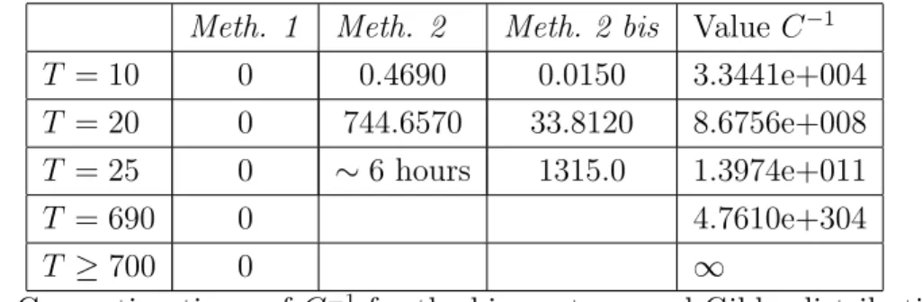
We present in Table 1 the times for the computation of C−1 for various values of T and
the following methods : (1) calculation of C−1 = E
1ATAT −2K1; (2) C−1 is obtained by
direct summation on ET using a simple loop, or using a bitmap dodge which computes
simultaneously the 2T elements of ET (2 bis). We stopped computing C−1 by summation
for T > 25.
Meth. 1 Meth. 2 Meth. 2 bis Value C−1
T = 10 0 0.4690 0.0150 3.3441e+004
T = 20 0 744.6570 33.8120 8.6756e+008
T = 25 0 ∼ 6 hours 1315.0 1.3974e+011
T = 690 0 4.7610e+304
T ≥ 700 0 ∞
Table 1 : Computing times of C−1 for the binary temporal Gibbs distribution with
parameters α = 1, β = −0.8.
We see that the computing times of C−1 = E
1ATAT −2K1 are negligible for T < 700 while
the summation method becomes quickly infeasible. Example 2 : bivariate binary temporal model
E = {0, 1}2 (N = 4 states), and Z(T ) is the anisotropic Ising model:
E1AT = AT(1, ·) is AT’s first row with AT(1, j) = exp{αxj+ βyj+ γxjyj}; A is of size 4 × 4
defined by A(i, j) = exp{αxj + βyj + γxjyj + δ(xixj + yiyj)}, and K1’s i−th component
equals Pz=(x,y)∈Eexp{αx + βy + γxy + δ(xxi + yyi)}. We computed C−1 in two ways,
first using the the powers of A i.e. C−1 = E
1ATAT −2K1, then using its diagonalization C−1 = E
1ATP DT −2P−1K1. We took parameters α = 1, β = −0.8, γ = −0.5, δ = 0.04.
We were able to calculate C−1 = 9.9491e + 006 for T = 430 and then stopped for larger
T since the software treats C−1 as equals infinity. The computing times are null for both
methods, which means that we get instantaneously C−1’s value, and the size of A is still
too small to distinguish computations using power or diagonalization of A.
4 General Gibbs fields
4·1 Temporal Gibbs fields
The previous results can be extended to general temporal Gibbs models. As an illustration, let us consider the following model, characterized by the energy:
UT(z(T )) = X s=1,T θs(zs) + X s=2,T Ψ1,s(zs−1, zs) + X s=3,T Ψ2,s(zs−2, zs).
The joint distribution π defines a bilateral Markov field with the 4 nearest neighbours system, and conditional distributions:
π(zt | zs, 1 ≤ s ≤ T et s 6= t) =
= Pexp{θt(zt) + Ψ1,t(zt−1, zt) + Ψ1,t+1(zt, zt+1) + Ψ2,t(zt−2, zt) + Ψ2,t+2(zt, zt+2)}
u∈Eexp{θt(u) + Ψ1,t(zt−1, u) + Ψ1,t+1(u, zt+1) + Ψ2,t(zt−2, u) + Ψ2,t+2(u, zt+2)}
= π(zt| zt−1, zt+1, zt−2, zt+2).
Z is also a Markov chain of order 2 with: π(zt | zs, s ≤ t − 1) = exp{θt(zt) + θ∗t(zt) − θt−1∗ (zt−1) + Ψ1,t(zt−1, zt) + Ψ2,t(zt−2, zt) + θ∗∗ t (zt−1, zt) − θ∗∗t−1(zt−2, zt−1)} = π(zt| zt−1, zt−2) where θ∗ t(zt) is given by (2·4) and θ∗∗ t (zt−1) = X uT t+1 exp{Ψ2,t+1(zt−1,ut+1) + Ψ2,t+2(zt, ut+2) + T X t+3 Ψ2,s(us−2,us)}.
For t ≤ T − 2, the conditional distribution π(z(t) | zt+1, zt+2, · · · , zT) depends only on
(zt+1, zt+2):
π(z(t) | zt+1, zt+2) = Ct(zt+1, zt+2) exp Ut∗(z(t); zt+1, zt+2),
where we name U∗
t(z(t); zt+1, zt+2) the future conditional energy:
Ut∗(z(t); zt+1, zt+2) = Ut(z(t)) + Ψ1,t+1(zt, zt+1) + Ψ2,t+1(zt−1, zt+1) + Ψ2,t+2(zt, zt+2), and Ct(zt+1, zt+2)−1 = X ut 1∈Et exp U∗ t(u1, .., ut; zt+1, zt+2).
For a, b and c ∈ E, it is easy to verify that:
U∗
t(z(t − 1), a; (b, c)) = Ut−1∗ (z(t − 1); (a, b)) + θt(a) + Ψ1,t+1(a, b) + Ψ2,t+2(a, c).
With the convention Ψ1,s ≡ Ψ2,s ≡ 0 for s > T , we define:
• for t ≤ T − 2, the vector Γt(z(t)) of the conditional contributions, conditionally to
the future (zt+1, zt+2) = (ei, ej), i, j = 1, N, by the N2× 1 vector of components (i, j):
γt(z(t); (ei, ej)) = exp Ut∗(z(t); ei, ej);
• ΓT −1(z(T − 1)), the vector of the contributions conditionally to the future zT = ei :
(ΓT −1(z(T − 1))i = exp{UT −1(z(T − 1)) + Ψ1,T(zT −1, ei) + Ψ2,T(zT −1, ei)};
• ΓT(z(T )) the constant vector of components exp{UT(z(T )}.
In the same way, we define the matrix A of size N2× N2 whose non zero components
are:
At((i, j), (k, i)) = exp{θt(ek) + Ψ1,t+1(ek, ei) + Ψ2,t+2(ek, ej)}
Like in section 3·2, we obtain a recurrence formula on the γt:
γt(z(t − 1), ek; (ei, ej)) = At((i, j), (k, i)) × γt−1(z(t − 1); (ek, ei))
together with the statement (3·4) on the contributions Γt(z(t)). In this context, (Zt, t =
1, T ) is a Markovian process with memory 2 and Yt= (Zt, Zt+1) a bivariate Markov chain
4·2 Spatial Gibbs fields
Let us consider Zt = (Z(t,i), i ∈ I), where I = {1, 2, · · · , m}, and Z(t,i) ∈ F (Zt ∈ E =
Fm). Then Z = (Z
s, s = (t, i) ∈ S) is a spatial field on S = T × I. We note again
zt= (z(t,i), i ∈ I), z(t) = (z1, .., zt) and z = z(T ).
Without loss of generality, we suppose that the distribution π of Z is a Gibbs distri-bution with translation invariant potentials ΦAk(•), k = 1, K associated to a family of subsets {Ak, k = 1, K} of S, ΦAk(z) depending only on zAk, the layout of z over Ak. Then
π is characterized by the energy: U(z) = X
k=1,K
X
s∈S(k)
ΦAk+s(z), with S(k) = {s ∈ S s.t. Ak+ s ⊆ S}.
For A ⊆ S, we define the height of A by H(A) = sup{|u − v| , ∃(u, i) and (v, j) ∈ A}, and H = sup{H(Ak), k = 1, K} the biggest height of the potentials. With this notation,
we write the energy U as the following:
U(z) = H X h=0 T X t=h+1 Ψ(zt−h, · · · , zt) with Ψ(zt−h, · · · , zt) = X k:H(Ak)=h X s∈St(k) ΦAk+s(z)
where St(k) = {s = (u, i) : Ak+ s ⊆ S and t − H(Ak) ≤ u ≤ t}.
(Zt) is a Markov field with the 2H-nearest neighbours system but also a Markov process
with memory H; Yt = (Zt−H, Zt−H+1, · · · Zt), t > H, is a Markov chain on EH for which
we get the results (3·5) and (3·6).
4·3 Computing the normalization constant for the Ising model
We specify here the calculus of C−1 in the case of a translation invariant potentials Ising
model (Kindermann and Snell (1980), Guyon (1995)). Let S = T × I ={1, 2, · · · , T } ×
{1, 2, · · · , m} be the set of sites, and F = {−1, +1} the state space. We consider Z =
(Z(t,i), (t, i) ∈ S) a Markov field on S with the four nearest neighbours system, a site
(t, i) being a neighbour of (s, j) if k(t, i) − (s, j)k1 = 1. The joint distribution π of Z is characterized by the singletons and pairs potentials:
Φt,i(z) = α z(t,i) for (t, i) ∈ S,
Φ{(t,i),(t,i+1)}(z) = β z(t,i)z(t,i+1) for 1 ≤ i ≤ m − 1,
Forgetting the spatial dimension, we consider the state zt = (z(t,i), i = 1, m) ∈ E = {−1, +1}m. Then Z is a temporal Gibbs field with the following translation invariant
potentials: θt(zt) = θ(zt) = α X i=1,m z(t,i)+ β X i=1,m−1 z(t,i)z(t,i+1), Ψt(zt−1, zt) = Ψ(zt−1, zt) = δ X i=1,m z(t−1,i)z(t,i), 2 ≤ t ≤ T.
Let us give some notations associated to c = (ci, i = 1, m) and d = (di, i = 1, m),
two states of E = {−1, +1}m; we first introduce n+(c) = ]{i ∈ I : c
i = +1} and n−(c) =
]{i ∈ I : ci = −1} (n+(c) + n−(c) = m), then v+(c) = ]{i = 1, m − 1 : ci = ci+1} and
v−(c) = ]{i = 1, m − 1 : c
i 6= ci+1} (v+(c) + v+(c) = m − 1), and finally n+(c, d) = ]{i ∈
I : ci = di}, n−(c, d) = ]{i ∈ I : ci 6= di} (n+(c, d) + n+(c, d) = m).
Since the potentials are invariant, the matrix At given by (3·2) does not depend on t,
we have At = A, t ≤ T − 1, the 2m× 2m matrix whose general term is,
A(a, b) = exp{α(n+(b) − n−(b)) + β(v+(b) − v−(b)) + δ(n+(a, b) − n−(a, b))}, a, b ∈ E. Moreover, for t = T, AT(a, b) = exp{α(n+(b) − n−(b)) + β(v+(b) − v−(b))}. Therefore, the
normalization constant of π is C−1 = E
1ATAT −2K1.
Since K1 is given by a summation over E = {−1, +1}m, and the size A is 2m× 2m, this
formula is practically useful for m not too big.
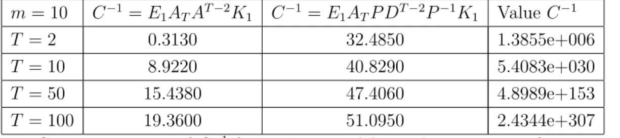
Example 3
Table 2 gives computing times for the normalizing constant for the Ising model above with parameters α = 0.15, β = 0.05, δ = −0.08. In the case T = m = 2, the model is the one given in example 2 with F = {0, 1}. We consider varying values of T and m = 10, that is we work with vectors and square matrices of size 210 but without theoretical constraints
on the size of T = {1, 2, · · · , T }. We compute C−1 using the powers of matrix A or its
diagonalization. m = 10 C−1 = E 1ATAT −2K1 C−1 = E1ATP DT −2P−1K1 Value C−1 T = 2 0.3130 32.4850 1.3855e+006 T = 10 8.9220 40.8290 5.4083e+030 T = 50 15.4380 47.4060 4.8989e+153 T = 100 19.3600 51.0950 2.4344e+307 Table 2: Computing times of C−1 for an Ising model on a lattice 10 × T for various T.
We observe that it’s computationally more efficient to compute the powers AT −2rather than
to use the diagonalization of A. Indeed, the diagonalization procedure itself is expensive for large size matrices.
4·4 Other generalizations
First, we presented the forward recursion for Gibbs distributions with singletons and pairs potentials. The results can be extended to larger potentials (triple or more).
Another extension is to consider variable state spaces. The recurrence (3·4) and prop-erties (3·5), (3·6) hold for different state spaces Et of the components Zt; in this case, the
associated matrices At involved in (3·6)are not necessarly square.
Finally, we can extend the results to embedded sets T ; for instance let us consider the de-creasing sequence T = SQ⊃ SQ−1 ⊃ · · · ⊃ S1 of parts of T = {1, 2, · · · , T }; similarly to the
former future-conditional contributions, we define the contributions γq(z(Sq); z(T Sq)),
conditionally to the outer layout z(T Sq). Let us give the following example: we assume
Sq = Sq−1∪ ∂Sq−1 for q = 1, Q − 1. Then, we obtain the conditional energy
Uq∗(z(Sq); z(∂Sq)) = Uq−1∗ (z(Sq−1); z(∂Sq−1)) + ∆q(z(∂Sq−1)); z(∂Sq))
with ∆q(z(∂Sq−1)); z(∂Sq)) =
P
u∈∂Sq−1θu(zu)+ P
u∈∂Sq−1,v∈∂Sq,<u,v>Ψ{u,v}(zu, zv). then we define the matrices Aq by
Aq(∂Sq; ∂Sq−1) = exp ∆q(z(∂Sq−1); z(∂Sq)).
As an illustration let us set the following decreasing sequence T = ST −1 = {1, 2, · · · , T },
ST −2 = {1, 2, · · · , T − 1}, · · · , S2 = {1, 2, 3} and S1 = {2}. For q = T − 1, · · · , 3, the
conditional contributions and the matrices A are defined in the usual way (3·1) and (3·2), while for q = 2, A2 is a N × N2 matrix with A2(z4, (z1, z3)) = exp{θ1(z1) + θ3(z3) +
Ψ4(z3, z4)}.
5 Conclusion
The technique proposed in this paper to evaluate marginals and normalisation constant is applicable to Markov chains, Markov fields. It overcomes the need to resort to approximate alternatives when one wants to evaluate the likelihood or the normalizing constant of a Gibbs field. It makes feasible the exact evaluation of the normalizing constant for moderate set of sites, eliminating any Monte Carlo procedure, variational scheme, or (approximate)
Bayesian computations steps. As a statistical consequence, it is therefore possible to per-form true maximum likelihood estimation for such Gibbs field. Another application is to allow exact simulation.
We gave several illustrations of computing times for the normalizing constant. For one dimensional two states Gibbs fields, we are able to compute instantaneously the normalizing constant for a sequence of length 700, as well as for a sequence with four states and of length 400. We could keep computing for bigger lengths using another software. However, our main goal here is to provide a new method and we let the users choose their way of programming.
For spatial processes, we have computed the normalizing constant for an Ising model on a lattice 10 × 100 in 20 seconds. Following the discussion above, we could increase T, one of the side of the lattice; the limitation of the procedure ensures from the manipulation of
Nm× Nm matrices. So the method seems to fail for large square lattices. As a comparison,
Pettitt et al. (2003) compute the normalizing constant for an autologistic model defined on a cylinder lattice for which the smallest row or column is not greater than 10. They suggest to split a large lattice into smaller sublattices along the smallest row or column. A similar idea could apply here.
References
F. Bartolucci, J. Besag, 2002. A recursive algorithm for Markov random fields. Biometrika 89 (3), 724-730.
J. Besag, 1974. Spatial interactions and the statistical analysis of lattice systems. J. Roy.
Statist. Soc. B 148, 1-36.
R. Kindermann and J.L. Snell, 1980. Markov random fields and their applications. Con-temp. Maths.
X. Guyon, 1995. Random Fields on a Network: Modeling, Statistics, and Applications. Springer-Verlag, New York.
G. Lovinson, 2006. A matrix-valued Bernoulli distribution. J. of Mult. Anal. 97, 1573-1585. M. Khaled, 2008. Estimation bay´esienne de mod`eles espace-´etat non lin´eaires. Ph.D.
The-sis, Universit´e Paris 1 http://mkhaled.chez-alice.fr/khaled.html
M. Khaled, 2008. A multivariate generalization of a Markov switching model. working
paper, C.E.S., Universit´e Paris 1 http://mkhaled.chez-alice.fr/khaled.html
J. Moeller, A.N. Pettitt, R. Reeves, K.K. Berthelsen, 2006. An efficient Markov chain Monte Carlo method for distributions with intractable normalizing constants. Biometrika 93, 2, 451-458.
A.N. Pettitt, N. Friel, R. Reeves, 2003. Efficient calculation of the normalizing constant of the autologistic and related models on the cylinder and lattice. J. Roy. Statist. Soc. B, 65 Part 1, 235-246.
R. Reeves, A.N. Pettitt, 1982. Efficient recursions for general factorisable models.