Acoustic Wave Backscattering In A Random Inhomogeneous Ocean Sediment

RANDOM INHOMOGENEOUS OCEAN SEDIMENT

Weiqun Shi

Earth Resources Laboratory

Department of Earth, Atmospheric, and Planetary Sciences Massachusetts Institute of Technology

Cambridge, MA 02139

ABSTRACT

The backscattering of sound by inhomogeneities of the ocean sediment may provide a remarkable effect on underwater acoustic wave propagation. It may also be used as a means of remotely estimating complicated sediment properties. In this paper, a theoretical model of acoustic waves backscattered from an inhomogeneous sediment is formulated based on the Born approximation. The model not only contains the formal homogeneous bottom case but is also extended to the more realistic stratified bottom case. A complex wavenumber, in which an attenuation coefficient is introduced, reveals significant changes of the penetration depth within the sediment.

The model predicts that for the stratified bottom, the backscattering strength is rapidly oscillating and decreases sharply at small grazing angles owing to the refraction of the waves caused by the sound velocity gradient.

In order to reduce the number of independent variables, Biot's theory is applied to relate three-dimensional density fluctuations to sound speed fluctuations through porosity. A transverse-isotropic model is also developed to access the three-dimensional sound speed fluctuation spectrum.

Geoacoustic surface and cross-hole tomographic data acquired from different sites characterizing sandy and silty bottoms are used to obtain three-dimensional sediment volume inhomogeneities. Backscattering strengths are evaluated for those bottom cases. The results agree with intuition and other published data.

INTRODUCTION

The investigation of acoustic backscattering from the ocean bottom began during World War II and has been carried out for a wide band of frequencies in many ocean regions of

the world (Alberts, 1967; Urick, 1967). A number of experimental data has revealed a complicated dependence of the backscattering strength on the incident wave frequency, grazing angle, interface roughness, and sediment volume inhomogeneities (e.g., Berson et aI., 1986; Jackson et al., 1986; Jackson and Kevin, 1992; Ivakin, 1986). Itis generally found that the backscattering strength (BS) has an average value of -30 dB and obeys the so called Lambert's law [i.e., BS cc sin2 (grazing angle)] over a wide range of te graz-ing angle. The backscattergraz-ing strength decreases sharply at small grazgraz-ing angles. There is poor dependence of the backscattering strength on frequency. Backscattering caused by sediment volume inhomogeneities is dominant in soft sediments, while backscattering caused by surface irregularities is dominant in sandy bottoms.

Along with the experimental studies, a great deal of theoretical research has been carried out on both bottom interface roughness and sediment volume inhomogeneities backscatterings. Many fine models of sediment volume scattering have been success-fully developed in the literature (e.g., Stockhausen, 1963; Zhitkovskii, 1968; Ivakin and Lysanov, 1981a,b, 1985; Tang, 1991). However, there are shortcomings in the existing models. First, most of the existing models have been based on the common assumption that variability of either sound speed or density variations exits only in one direction (e.g., vertical direction). This simplified 2-D treatment is limited to a stratified lay-ered sediment. In many ocean regions, however, sound velocity and density variations can also exist along the horizontal direction. It is necessary to develop a model that can properly address complicated three dimensional sediment variations. Second, when solving for the scattering field, most of the existing models used the small perturbation theory about a homogeneous medium, which has a nonvarying sound speed profile with depth. Such a simple model is justified in the case of high frequencies, when the incident waves can only penetrate into a top thin layer of the sediment owing to the strong at-tenuation of sound in the sediment. As the frequency decreases, the penetration depth increases so that the bottom stratification cannot be ignored.

The purpose of this paper is to investigate backscattering of acoustic waves from a sediment containing volume inhomogeneities of sound speed and density. A model is created which attempts to address the above shortcomings by including a linearly-increasing sound speed profile within the sediment, and three-dimensional fluctuations in both sound speed and density.

THEORY OF ACOUSTIC WAVE BACKSCATTERING IN

INHOMOGENEOUS MEDIA

In general, the numerical approaches applied in solving the scattering field today are based on important theoretical developments within the field of wave propagation over the past decades. Of particular importance are the various assumptions and approxi-mations made in order to solve realistic propagation problems. The inhomogeneities we discuss paper are caused by density and sound speed fluctuations. Following this idea, we apply the first-order Born approximation and the method of small perturbation with

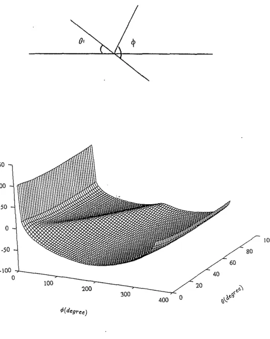
associated boundary conditions to solve for the scattered field. The method is limited to a single scattering caused by small fluctuations within the medium. Figure 1 shows the schematic diagram of the media. The acoustic source and receiver are located above the random medium. In ocean acoustics, they are usually located in the water column. We define the grazing angle and the incident and scattering angles of the inhomogeneous volume, as shown in the figure.

Homogeneous Medium

The medium is first assumed to be homogeneous on the average, i.e., the mean values of the density and the acoustic velocity are constants. The acoustic wave field P of a point source in a medium with variable sound speed C and density P obeys (Chernov,1960;

Aki and Richards, 1980):

1 w2

p'V. (-'VP)

+

2'P=-41fo(x-xo). (1)

P c

Assume there are small random fluctuations of density and sound velocity which make them deviate only slightly from their mean values,

C

=

Co

+

8c,

<

OC

>=

0 P

=

Po

+

op,

<

op

>=

O.

(2) (3) The terms 8c and 0P are the random functions of the coordinates and are assumed to be much smaller than the mean values Co and Po. Under these perturbations, the total acoustic wave field can be treated as consisting of two parts-a primary wave Po satisfying the unperturbed condition with On

=

_{0, and a scattered wave Ps generated} by the interaction between the primary wave and the inhomogeneities:

P

=

Pp +Ps.

Defining the wave number k

_o,

(4)

k

_o

= w/co (5)

and substituting (4) into the original wave equation, and neglecting the second and higher order terms yields:

2 2 20C 20P op

'V Ps+koPs=2ko-Pp+ko-Pp+'V'(-'VPp) (6)

Co Po Po

The scattered wave field is then obtained by the integral of a Green's function with the right-hand side of equation (6).

Ps(x) = -41

1

G(x, X)[(2oc(x')

+

op(x') )k6 Pp(xo,

x')+

'V'.(op(x')'V'Pp(xo, x'))]d3_{x' (8)}

We know for a point source, Pp and G give the solution: eiko]x'-xol Pp(xo,x' )

=

I

I

I

0 x -Xo eikolx-x'l G(x,x' )=

I

_x-x

'I

(9) (10) Assume that the. characteristic linear dimension of the scattering volume is large com-pared to the spatial scale of inhomogeneities and small comcom-pared to the distance of the source Ixol and the receiver Ix'l from the origin of the coordinates located within the scattering volume. Mathematically this means:

Ix' - xol =

JX

l2

+

X5 -

2x' · Xo "" Ixol

+

koki·

x' Ix - xii =

Jx

2

₊

X '2 - 2x· x' "" Ixl-

kok

s 0x', therefore, (11) (12) (13) where,

k

i is the unit vector in the incident wave direction, k~ is the unit vector in the

scattered wave direction, and

6.k

is the difference between the incident wave direction and the scattered wave direction:

(14)

(15) Equation (13) states that the scattered field is made up by two parts-the sound velocity fluctuations which is the first term in the bracket, and the density fluctuations which are the second and third terms in the bracket. Since the fluctuations of the sound speed and density that appeared in the above equations are random functions of the coordinates, they require a transition to ordinary functions by multiplying the complex conjugate and then taking the statistical average:

<

IPs(xW

>=

(41fI~flxol)2

<

IJI

2

>,

where J is defined as:

J = f[2oc(x' )

+

op(x' ) _

k

s •

k

iop(xl)]e-ikol>koX'd3xl

J

v Co Po Po

(16) In order to quantify the scattering properties of the ocean bottom, a parameter called scattering cross-section per unit volume IJ"v (or scattering coefficient _{m v )} is defined by

the formula (Brekhovskikh, 1960):

Wscat

(Tv =m_v =

(18)

in whichWseatis the average acoustic power scattered by a volumeV of the bottom in a

specified direction per unit solid angle, and line is the intensity of the incident acoustic

wave near the scattering volume. According to this definition, we obtain:

1 k5 2 2

(Tv

=

V(47f)

<

IJI

>.

In addition to (Tv, a so-called scattering cross-section per unit area (Ts, that is

dimen-sionless, is often used in acoustic measurement:

as = (jvd

where d is the equivalent depth of penetration.

Stratified Medium

General form

(19)

In the previous section, the bottom was assumed to be homogeneous on the average, i.e., the mean values of density and sound velocity did not depend on the depth. Such a simple model is justified in the case of high frequencies, when the incident waves can only penetrate a thin layer at the top of the sediment owing to the strong absorption of sound in the sediment. For lower frequencies, the penetration depth increases and the bottom stratification cannot be ignored. For this kind of ocean bottom, the unperturbed density and sound speed are functions of depth,

c = co(z)

+

Dc. p= Po(z)

+

5p

(20) (21) The primary wave field Pp and the Green's function G inside the scattered wave integral

(8) should satisfy the following wave equations: \72pp(XO'x')

+

k5(z)Pp(xo, x') = -47f5(xo - x')

\72G(x,x' )

+

k5(z)G(x,x' )= -47f5(x - x') where ko(z) = wjco(z). (22) (23) (24)

In general, it is not easy to find analytical solutions for equations (22) and (23). However, ifk(z) is assumed to be slowly varying with the depth, the solutions ofPpand G may be represented by their corresponding solutions in a homogeneous media slowly modulated by an envelop function that depends on depth, i.e,

G(x,x' )

=

GO(X,X')g(Z) where eikolxo-xlJ Po(xo,X') = [ '[ Xo - x eikolx-x'l GO(X, x')

= [

_x-x

'[ .

(26) (27) (28)

Ifthe scattering volume's vertical height is very small compared to that of the horizontal cross section, and the horizontal cross section is very small compared to the distances between the scattering volume and the source and receivers, then the source and the receiver can be assumed to be located in the far field. Therefore the solutions have simple forms:

(29) (30) where, ~i,xis are the horizontal components of the incident and the scattered wave numbers, respectively, and xref

=

[rref'OJ is a reference point on the surface of the scattering volume. Substituting the above approximations into the Helmholtz equations (22), (23) and using the separation of variables, we obtain the following equations:

\72p(z)

+

[k5(Z) - ~l]p(z) = 0

\72g(z)

+

[k5(Z) - ~;]g(z) =

o.

Then, the associated scattering field is:

where

(31) (32)

(33)

(34) N(r,z) is the term associated with density and sound speed fluctuations, as described in the previous section. After making a few simple transformations, the scattering cross-section per unit area is obtained as a function of depth-dependent g(z),p(z),

where, av(z) can be seen as the scattering cross-section per unit volume determined by the local mean sound velocity and fluctuation, defined by the previous section. And H

is the thickness of the sediment layer. Averagingav over the depth, we get,

(36)

where itv is called the effective (depth-averaged) volume backscattering cross-section

of the ocean sediment. It states that the total sediment backscattering cross-section is perturbed by the depth-dependent function g(z),p(z). The value of the scattering cross-section not only depends on the sediment volume inhomogeneities, but also on the sediment stratification. Comparing to equation (19), one notices the equivalent depth of penetration dis now expressed in terms of the integral ofg(z),p(z), i.e.,

d

=

foH

Ig(z)p(zWdz.

For backscattering, we have p(z) = g(z), therefore,

d=

foH

Ig(zWdz.

(37)

(38) Linearly increasing bottom

The most common case of the stratified medium is when the acoustic parameters of the medium are increase linearly along the depth. In reality, the ocean environment is a combination of the two: a water column and a sediment column. The numerical approaches have to include the boundary conditions. The acoustic velocity for this situation is given by:

{

CO in the water

c(z) = co(1

+

az/2) in the sediment'

Assuming (az) is very small, and introducing a small attenuation into the sediment layer (restricted to reasonably low frequency, the attenuation in the water column is ignored), the wave number is expressed as

k( ) _ { ko in the water

z - (k_o

+

i7))(1 - az)1/2 in the sediment'

7) is the attenuation coefficient of the compressional wave through the sediment. Rogers, et al. (1993) measured the attenuation coefficient and found that 7) depends on frequency:

7)= 6.336f1.144(10-6). (39)

Let g1(Z) represent g(z) when z

<

O. Let g2(Z) represent g(z) when z

>

O. The Helmholtz equations for g1 and g2 and the boundary conditions are:

(41) Equation (41) can be reduced to an Airy equation by introducing independent complex variables

t,

Zt and 0: where

t

=

Z - Zt

o

1 - e(ko

+

i'f/)-2 Zt = a

The general solutions for (40) are:

The general solutions for (41) are: A.(Z - Zt) B.(z - Z') 't {j ,1. 8 ' (42) (43) (44) (45) (46) (47)

where Ai(t), and Bi(t) are the Airy functions). The proper choice of Airy functions is suggested by the ray theory. After a ray penetrates deep enough into the sediment, it becomes horizontal as a result of refraction caused by the sound speed gradient and is then redirected upward to meet the water/sediment interface. The depth (denoted asZt), where a ray becomes horizontal is called the turning depth, for which the bracketed term in equation (41) vanishes. Translating from ray to wave predictions, one expects the solution of equation(41) to represent a standing wave forZ

<

Ztand decay quickly toward

zero as Z --+ 00. It follows from Breknovskikh (1960) that when t is a complex variable,

only the solution Ai(t) satisfies this requirement. Therefore, taking into account:

and

() iVk'-<2.

+

R -iVk2-'2z

g z = e o"~ e O " , _(Z

<

0) (48)

Z - Zt

g(z) = TAi(-o-)' (Z

>

0) (49)

where, R is the reflection coefficient and T is the transmission coefficient. RandT can be obtained by the boundary conditions:

(51) (54) so we can get: 2 T

=

'( ., .

(52) A ( 3.)

+

A; --,r) i - <5 i6J k

2-e

Substituting into equation (38), the equivalent depth of penetration is obtained:

d

= 16[A;(- Zt)

+

Ai(--¥-)

1-4

r

H[A;(Z -

z')1

4

dz.

(53)

8

i8Jk5-~2

J

o

8

Since the attenuation has already been introduced in the above derivation, the upper limit (H) of the integral can go to infinity 00.

CORRELATIONS BETWEEN DENSITY AND VELOCITY

FLUCTUATIONS

In the previous sections, the scattered field has been described by two independent random variables,

&1

Co and 8P

1

Po. Since existing experimental data can only provide one of these properties, it becomes necessary to reduce the number of independent variables by the use of an approximation. A common method (Tappert, 1991a) is ·to employ the equation:

8p

&

- = 2(r

-1)-Po Co

wherer is usually in the range between 1 and2according to statistical results (Winokur, et al., 1983). This paper will apply Biot's theory to model the physical properties of the sediment.

For a saturated sediment, according to Biot's theory, the bulk density Pis given by,

(55)

(56)

where Pr is the density of the grain material, Pf is the density of pore water, and

f3

is porosity, respectively. Similarly, the bulk modulus of the skeleton frame is given by (Yamamoto, 1983):

...!...=..E..+

1

_-/3.

K K_f Ks

Since the bulk modulus of the grain Ks is very large compared to the bulk modulus of

waterKf' the sound velocity can be approximated as:

(59) (58)

(62) (61) (60) The above equations build a relationship between density and sound velocity. Differen-tiating both the right and left sides of these equations, one can obtain:

!:J.p 2D!:J.c

-

-Po I- Dco where D is expressed as:

D= Pr-PI -1

Pr(1 (3:0)

+

PI

and define

1 D A A

r

=

1 _ D - 1-D k ,. ki .

Substituting them into equation (13), we obtain: k2eikolxoleikolxlr

J . .

8c(x')

P,(x)

==

0 e-,koD.k.x' _ _ d3x'

47flxllxol c o '

Now, the total sediment volume inhomogeneity is represented by only one independent variable-sound velocity fluctuation.

r

is a function of the density of the grain material, the density of the pore water, the mean porosity of the sediment, and the directions of the incident and the scattered waves. Since Pr, PI,(30 are the constants for a certain geophysical province, if the incident and scattering wave directions are known,

r

will be a constant for that province. Multiplying P, by its complex conjugate, and averaging over the ensemble of realizations of the medium, we get:

<

IP,12

>= (

kfir )21.N(q)e-ikOD.k'Qd3x'd3xll

27flxllxo

I

v

where N(q) is the autocorrelation function for the velocity fluctuations and is defined as: 8c(x')8c(x") N(q)

=<

2

>

Co (63) and q=x'-x". (64)

The double integral over the scattering volume V can be evaluated by integrating over the center-of-mass coordinate. Since the functionN(q) rapidly tends to zero at

Iql

»

I,

, (note,l, is the spatial scale of inhomogeneities), the limits of integration over q can be taken as -00 and +00. Using the Wiener-Khinchin Theorem (Tappert, 1991b), one obtains:

<

IP,1

2

_>=

_{27fkgr2V(lx llxol)-2S(!:J.k)}

where, S(k) is the 3-D power spectrum of the relative sound speed fluctuations.

S(k) - 1

1+

00 8c(x) 8c(x

+

x') -ik.x'd3 '

- - -

< - -

>e

x. (27f)3 - 0 0 Co Co (65) (66)

TRANSVERSE ISOTROPIC SPECTRUM OF VELOCITY

FLUCTUATIONS

In cylindrical coordinates, the 3-D power spectrum of the relative sound velocity fluc-tuations S(k) _{is denoted by S(kh', kv), where k h is the wave number vector in the}

horizontal direction, and k v is the wave number in the vertical direction. Making the assumption that the surfaces of S(kh, kv) are ellipsoids of revolution about the vertical axis (Tappert, 1991), meanS mathematically that,

(67)

and

(68)

(Y is the ratio of the horizontal to the vertical scale. Using this form with the recent

experimental measurements reported by Yamamoto et al. (1992a,b), a complete three-dimensional power spectrum of sediment volume sound speed fluctuations, named a 'transverse-isotropic spectrum', can be obtained and is used in this paper:

(69) Three parameters in this equation must be measured or estimated for every geological province. They are: 'Y, the spectral exponent; E, the structure constant; and (Y, the

aspect ratio. The scattering cross-section is then expressed as:

(70)

Letting 8 denote the grazing angle and ¢ denote the scattering angle, as shown in Figure 2, one can find:

I~kvl =

kol

sin(8)

+

sin(¢ - 8)1

I~khl = kol cos(8) - cos(¢ - 8)1

(71) (72)

then a typical scattering cross-section as a function of ¢ and 8 for ¢

=

0° -> 360°;

8

=

0° -> 90° is found and shown in Figure 2.

Note that the scattering cross-section has a minimum value when ¢ tends to 180°,

which is the angle that refers to the backscattering. When ¢ tends to zero, the angle that refers to the forward-scattering, the scattering cross-section goes to infinity. This result shows that the power spectrum formula (69) cannot properly address the forward scattering problem.

BACKSCATTERING STRENGTH

For the backscattering problem, the direction of the scattered wave is opposite to that of the incident wave, which gives

and

k

s

·ki=-1

L'lk

=

k_{s -} ki

=

-2ki

=

_-2ko

ki.

(73)

(74)

(75)

Thus the backscattering cross-section per unit volume is obtained:

Uv

=

2?Tkllr2S( -2koki).

The backscattering strength is defined as the following:

BS

=

10loglOUs

=

10logIO[27Tkllr2S( -2koki)d]. (76)

For the stratified medium, the equivalent depth of penetration is given by (38). For a homogeneous bottom, it is determined by the ray theory:

H .

B

d

=

sinBr { e-2_",xdx

₌

_{sm r(1-e-}2_{",£) (77)}

J

o

2o:s

where L is the travel distance through the sediment and is also determined by the ray theory.

B

r is the refraction angle. O:s is the attenuation coefficient in dB / m of

the compressional wave through the sediment. The relationship between O:s and the

previous defined 7J is,

=

-...!L =

6.336

₁

1.144(10-6 )

O:s 8.68 8.68 (78)

The range of frequency

1

is chosen between 50-600 Hz. Ifthe acoustic source and the receivers are located in the water column, we need to include the transmission loss of the water/sediment interface into the model, i.e,

(79)

whereT12 ,T21 are the transmission coefficients of the water/sediment interface.

NUMERICAL EVALUATIONS

Tomography DAta

To characterize random fluctuations in sediment, surface, and cross-hole tomography, experiments were carried out at different sites. The cross-hole tomographic data were collected from Chiba and Ohmiya in Japan (Yamamoto, et al., 1991) . These sites were once under water in Tokyo Bay and remain saturated. The cross-hole distances ranged

from 66 meters to 138 meters. The depth of each hole is 60 meters. The compressional wave velocity data are given on a 41 x 41 mesh with a sampling interval from 1.5-3.4 meters.

Cross-section I is located at Chiba I, site 1. This cross-section is 60 meters wide, 66 meters long, and begins about 5 meters below the sediment surface. Figure 3 shows its sound velocity tomography. There is a low velocity zone (1450-1550 mlssilty clay) widening from 20 meters to nearly 40 meters in depth. High velocity zones (1600-1730 m/s) containing soft sand intermixed with low velocity zones predominant the upper and lower layers. The mean compressional wave velocity is about 1583 mis, and the velocity gradient is found to be zero, which are both given in Table 1.

Figure 4 shows sound velocity tomography data from cross-section II located at Chiba II, with a width of 137 meters and a depth of 60 meters. At depths between 10 to 45 meters, one finds very soft silty clay with average velocity lower than 1500 m/s. The surface and the bottom layers are characterized by soft sand. The mean velocity and the velocity gradient of this section are also shown in Table 1.

Cross-section III, 71 meters wide and 60 meters deep, is located at Ohmiya. This experimental site is characterized by soft sand with an average velocity approximating

1581 m/s. Figure 5 shows its sound velocity tomography. One sees the fast sand layer increasing in dominance from upper the center layer to the bottom layer.

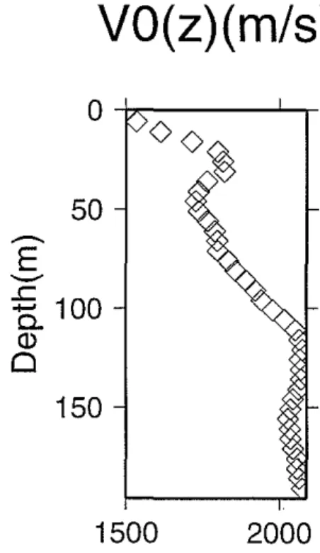
A surface tomography experiment was carried out at the North Atlantic continental shelf in New Jersey (Rogers et al., 1993) . The experiment was conducted by towing a newly developed seismic survey system-"Kite"-through the water. "Kite" can produce high-resolution three-dimensional images of subseafloor geology by arranging a hydrophone array with its axis perpendicular to the direction of motion through the water. Using compressional wave velocity profiles over depth provided by processing the arrival signals from a low frequency wide-band source, and superposing them with the data from high frequency source, the velocity distribution can be obtained. Figure 6 gives a velocity tomography collected by the "Kite" system from the North Atlantic continental shelf in New Jersey. The profile reveals a clear linearly-increasing layered structure of that area. The average gradient of the sound speed is about 2.4 (lis). Power Spectrum of Velocity Fluctuations

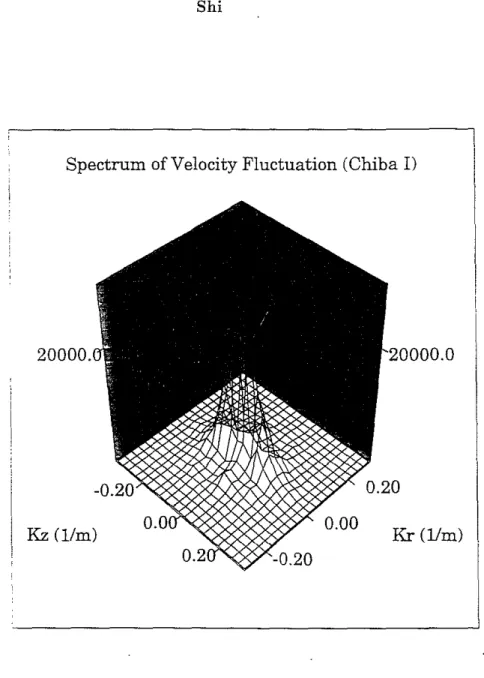
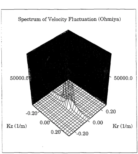
The corresponding power spectra of the relative sound speed fluctuations for the four cross-sections are calculated and shown in Figures 7-10. The numerical values of the spectral exponent I, the structure constant B, and the aspect ratio a are listed in Table 2. It is clear that the power spectrum has a power-law wavenumber dependency. The horizontal variation of the compressional velocity is weaker compared to that of the vertical variation. Nonlinear data fitting techniques give the numerical values of 1.2, 2.0, 2.954e-3 for I,a and B, respectively, at cross-section Chiba1.

Similarly, the numerical values of 1.0, 3.0, 8.7e-4 for I,a, and B, respectively are given for cross-section Chiba II. It is important to note that those two power spectra have a power-law exponential greater than -2, a value which is generally found for

most power spectra of bottom surface roughness (Brekhovskikh and Lysanov, 1982). This will cause strong bottom interaction, which means the scattered wave generated by volume fluctuations could be stronger than the roughness scattered wave.

The power spectrum of cross-section Ohmiya has the power-law exponent of -2.2. This sandy bottom is predicted to have weaker volume backscattering (Jackson and Kevin, 1992).

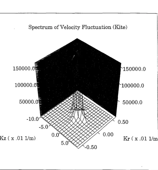
The power spectrum of the "Kite" data shows stronger variations in the vertical direction than in the horizontal direction. The corresponding values of'Y, E, and a are also shown in Table 2.

Calculation of Penetration Depth

For the stratified bottom, the equivalent depth of penetration d is a function of the grazing angle

e,

the incident wave frequency

f,

the gradient of sound velocity g, and the attenuation coefficient 'I) of the propagating compressional wave.

Equation (53) shows that both the amplitude and the integral part of d involve the Airy function, and, therefore, they reveal fast oscillation features at a small grazing angle (Figure 11). Each plot compares two cases-one with sediment attenuation (heavy line), and the other with sediment attenuation set to zero (light line).

In Figures 12 and 13, three frequencies are combined with two sound speed gradi-ents to reveal the penetration depth dependence on these parameters. Each plot also compares two cases-one with sediment attenuation (heavy line), and the other with sediment attenuation set to zero (light line).

Itis found in general, that at small grazing angles, the penetration depth is relatively unaffected by sediment attenuation. As the grazing angle gets larger, a significant reduction of the penetration depth is caused by the attenuation. For example, in Figure 12,when the frequency equals 200 Hz at 90 degrees of the grazing angle, the penetration depth in the case of non-attenuation can go to 10,000 meters, but the penetration depth in the case of attenuation is limited to 1,000 meters.

When the grazing angle is less than 35 degrees, the penetration depth is found to oscillate quickly. The oscillation period varies with frequency and sound speed gradient. At small grazing angles, the penetration depth decreases sharply toward zero. Since the the total backscattering cross-section is the product of the mean volume backscattering cross-section and the penetration depth, the behavior of the penetration depth strongly influences the total backscattering strength.

The penetration depth is frequency and sound speed gradient dependent. When attenuation is introduced, higher frequencies cause less penetration. For example, in Figure 12, under the same velocity gradient (2.4 l/s), 200 Hz waves can penetrate only to about 1,000 meters, but 100 Hz waves can penetrate to about 2000 meters. Under the same frequency but with a different velocity gradient, a larger gradient causes more penetration.

Backscattering Strength Evaluation

The backscattering strength versus incident the grazing angle of each experimental site is calculated and shown in Figure 14s-17.

The site of cross-section Chiba I was composed of silty clay. Figure 14 shows its backscattering strength as a function of the grazing angle. The backscattering strength level is approximately -30 to -20 dB in the angular range 20° to60°. For small grazing angles, the backscattering strength decreases sharply. Such strong backscattering results for a silty bottom and the tendency at small grazing angles agree with published data (Jackson and Kevin, 1992).

Backscattering strength is also found to be frequency dependent for this cross-section. The result shows that the backscattering strength at 200 Hz is slightly higher than at 100 Hz. Note in equation (69), the dependence of(Iv on frequency

f

is:

(80) Therefore, over the range 1

<<

'Y

<<

2, higher frequencies have stronger backscattering. Cross-section Chiba II (Figure 15) provides another example of an acoustically "soft" silty bottom. The backscattering strength is comparable to that of cross-section Chiba

1. This bottom also shows strong volume backscattering.

The bottom at the cross-section Ohmiya site is composed of soft sand. It was pre-dicted that scattering from a "harder" bottom such as this sandy bottom was mainly due to bottom surface roughness inthe range of grazing between 20 to 60 degrees (Jack-son and Kevin, 1992). The calculation presented in Figure 16 shows agreement with the results of other investigators. The mean backscattering strength level is about 10 dB less than that of silty bottoms. It is also interesting to notice that the frequency dependency disagrees with the first two cross-sections. The reason is that the expo-nential coefficient 'Y is larger than 2. For such an exponent, higher frequency causes weaker backscattering. Such inverse frequency dependence was also observed by other researchers (Preston and Akal, 1990). Another aspect that differs from the Chiba site is that the backscattering strength curve oscillates at small grazing angles. The effect is due to the linearly increasing sound velocity profile (Figure 5).

Velocity data from the "Kite" experiment also indicates a linearly increasing sound speed profile within the sediment (Figure 6). The backscattering strength is calculated based on the theory for a stratified bottom and is plotted in Figure 17. Curves represent-ing three frequencies: 100 Hz, (line), 200 Hz, (circle), and 500 Hz, (diamond), indicate that, in the range of small grazing angles, higher frequencies cause stronger backscat-tering. As the grazing angle gets larger, the low frequency scattering dominates the high frequency scattering. This behavior has been found by Zhitkovskii (1968) in the Atlantic continental slope and the continental rise.

For relatively small grazing angles, the backscattering strength reveals a rapid oscil-lation. The backscattering strength tends to zero sharply as the grazing angle decreases. The mean value of backscattering strength calculated for this velocity profile reveals a fairly weak backscattering in such bottoms. The reason for such low backscattering

strength might be the intrinsic limitation of the "Kite" system in measuring small-scale bottom fluctuations.

CONCLUSIONS

A theoretical model of acoustic waves backscattered by the ocean bottom was derived. In the model, scattering is caused by three-dimensional fluctuations in sediment density and sound velocity. Biot's theory is used to relate density and sound speed fluctuations through porosity, so that sediment volume inhomogeneity can be described by only one independent variable (sound speed fluctuation). Sediment attenuation is also included in this model, which affects the penetration depth. A complete mathematical derivation based on the small perturbation theory is given to evaluate the volume backscattering strength.

The model considers two bottom cases: (1) backscattering from an ocean sediment which has random fluctuations in sound speed and density but whose mean values remain constant; and (2) backscattering from random fluctuations in a sediment with linearly increasing sound speed profile.

Geoacoustic tomography and "Kite" data acquired from different sites are used to obtain measured three-dimensional sediment volume inhomogeneities. A transverse-isotropic model is developed to evaluate the three-dimensional sound velocity fluctuation spectrum.

Backscattering strength is found to be oscillating at small grazing angles in the case of stratified bottom. As the grazing angles decrease to zero, the backscattering strength decreases sharply. A complicated frequency dependence of the backscattering strength is found. When attenuation is introduced, a weaker backscattering at higher frequencies due to the stronger absorption inside the sediment is found. Backscattering strength calculations for different types of sediment agree with intuition and other published data. The results suggest that sediment volume scattering is dominant in soft bottoms and weaker in harder bottoms.

REFERENCES

Aki, K., and Richards, P.G., Quantitative Seismology, (Theory and Methods), Freeman, 1980.

Alberts, V.M., Underwater Acoustics, Vol. 2, Plenum Press, 1967.

Berson, J.M., Kloosterman, H. J., Akal, T. and Berrou, J. L., Directional measure-ments of low-frequency acoustic backscattering from the sea floor, in Ocean Seismo-Acoustics: Low Frequency Underwater r Acoustics, Akal, T. and Berson, J. M. (eds.), 327, Plenum, New York, 1986.

Brekhovskikh, L.M., Waves in Layered Media, Academic Press, 1960.

Brekhovskikh, L. and Lysanov, Y., Fundamentals of Ocean Acoustics, Springer-Verlag, 1982.

Chernov, L.A., Wave Propagation In A Random Medium, McGraw-Hill Book Co., 1960. Ivakin, A.N., Sound scattering from ocean bottom: Theory and experiment, Ocean

Seismo-Acoustics, 521, Plenum Press, 1986.

Ivakin, A.N. and Lysanov, Y.P., Underwater sound scattering by volume inhomogeneities of bottom medium bounded by a rough surface, Sov. Phys. Acoust., 27, 1981a. Ivakin, A.N. and Lysanov, Y.P., Theory of Underwater Sound Scattering by Random

Inhomogeneities of the Bottom, Sov. Phys. Acoust., 27, 61, 1981b.

Ivakin, A.N. and Lysanov, Y.P., Backscattering of sound from an inhomogeneous bottom at small G, Sov. Phys. Acoust., 31, 263, 1985.

Jackson, D.R., Baird, A.M., Crisp, J.J., and Thomson, P.A.G., High-frequency bottom backscattering measurement in shallow water, J. Acoust. Soc. Am., 80,1188, 1986. Jackson, D.R and Kevin, B.B., High-frequency bottom backscattering: Roughness

ver-sus sediment volume scattering, J. Acoust. Soc. Am., g2, 1992.

Preston, J.R and Akal, T., Analysis of Backscattering Data in the Tyrrhenian Sea, J.

Acoust. Soc. Am., 87, 119, 1990.

Rogers, A.K., Yamamoto, T., and Carey, F., Experimental investigation of the sediment effect on acoustic wave propagation in the shallow ocean, J. Acoust. Soc. Am., g3, 1747,1993.

Stockhausen, J.H., Scattering from the volume of an inhomogeneous half-space, NRE. Report, 63/9, 1963.

Tang, D., Acoustic wave scattering from a random ocean bottom, Ph.D. thesis, MIT, 1991.

Tappert, F.D., Models of scattering from sediment volume fluctuations, notes, March, 1991a.

Tappert, F.D., Geophysical model of sub-bottom volume fluctuations of sound speed, notes, March, 1991b.

Urick, RJ., Principles of Underwater Sound for Engineers, McGraw-Hill, 1967.

Yamamoto, T., Acoustic propagation in the ocean with a poro-elastic bottom, J. Acoust. Soc. Am., 73, 1983.

Yamamoto, T., Nye, T., and Kuru, M., PRBS P2_{S cross-hole tomography experiment}

Chiba, RSMAS, G.A.L. Report, 1992a.

Yamamoto, T., Nye, T., and Kuru, M., PRBS P2_{S cross-hole tomography experiment}

II-KSC Ohmiya, RSMAS, G.A.L. Report, 1992b.

Yamamoto, T., Turgut, A., and Schulkin, M., Geoacoustic properties of the seabed sediment critical to acoustic reverberation at 50 to 500 Hz, RSMAS, G.A.L. Report, 1991.

Zhitkovskii, Y., Sound scattering by inhomogeneities of the ocean bottom, Izv. Akad. Nauk SSSR Fiz. Atm. Okeana,

4,

567, 1968.

Site Width(m) Depth(m) Mean Velocity (m/s) Velocity Gradient(l/s)

Chiba I 66 60 1583.1

o.

Chiba II 137 60 1560

o.

Ohmiya 71.4 60 1582 2.5

Kite 3840 200 1766.3 2.4

Table 1: Statistical Geoacoustic Parameters of Each Site

parameter Chiba I Chiba II Ohmiya Kite Data B 2.95E-3 8.7E-4 2.86E-4 2.1E-7

a 2.0 3.0 2.67 13

'Y 1.2 1.0 2.4 1.0

sourse,resource

grazing angle

Figure 1: Schematic diagram of the medium.

200 ¢(d_{egree )} 300 400

o

20 80 100

Velocity Tomography

VQ(z)(m/s)

o

-.20

E

...-..c:

-

Cl.. Q)

o

40

60

o

25

50

Range(m)

-.20

E

...-..c:

-Cl.. Q)

o

40

1500

2000

I

·'W;M;l:i~

1450

Velocity (m/s)

1600

Velocity Tomography

VO(z)(m/s)

1500

~A

&~

60

...1-~----r,....L

2000

. - 20

E

...-.r:::

-0.. Q)

0

₄₀

125

100

50

75

Range(m)

25

o

60

o

. - 20

E

...-.r:::

+-' 0.. Q)

o

40

1>5illJ~{~f~j~

1450

Velocity(m/s)

1600

Velocity Tomography

VQ(z)(m/s)

:>

.- 20

.-

20-E

E

...

...

..c

_...

..c

_...

0.. 0.. CD CD

o

40

o

40-

-60

o

25

50

Range(m)

1500

2000

I

';{{;i~l~

1450

Velocity (m/s)

1800

Velocity Tomography

VQ(z)(m/s)

50

50

...-.

...-.

E

E

---

---:5

_0-

100

:5

_0-

100

eD eD

0

0

150

150

o

-!---I.-7 7 + ' ' ,

-2000

1500

o

-I,.,----...L...,--50

100

150

200

Range(m)

o

2000

Velocity(m/s) 1 - - 1

----"='ii~=_~

1500

Spectrum of Velocity Fluctuation (Chiba

1)

20000.

Kz (lim)

Figure 7: Power spectrum for cross-section Chiba1.

20000.0

Spectrum of Velocity Fluctuation (Chiba

II)

20000.

Kz

(11m)

Figure 8: Power spectrum for cross-section Chiba II.

20000.0

Spectrum of Velocity Fluctuation (Ohmiya)

50000.

Kz (lim)

Figure 9: Power spectrum for cross-section Ohmiya.

50000.0

Spectrum of Velocity Fluctuation (Kite)

150000.

100000.

IKz (

x .01llm)

Figure 10: Power spectrum for "Kite" data.

150000.0

100000.0

50000.0

Amp. of d

4

Q.

~

2

o

~?~;--r----1~:::::;===r==l-o

10

20

30

40

50

60

70

80

90

Int. Part of d

4

"1:l

-

a 1:::

~

2

...:

£:

0-+==----,.-....,.----,-...,....-,...---,...-.,----..,..-+

o

10

20

30

40

50

60

70

80

90

Grazing Angle(degree)

d=Penetration Depth,(grad.=O.8)

4

~ "0 ~ (!'

2

0

..J

f=100Hz

0

4

~ "0 ~ (!'

0

2

..J

f=200Hz

0

4

'C

_~ (!'

2

0

..J

f=SOOHz

0

0

10

20

30

40

50

60

70

80

90

Grazing Angle(degree)

d=Penetration Depth,(grad.=2.4)

4

o

4

o

4

o

-- f-,

I

f=lOOHz

I

-

--- f-f=200Hz

,

,

,

,

,

,

,

,

~

- f-f=500Hz

,

,

,

,

,

,

,

o

10

20

30

40

50

60

70

80

90

Grazing Angle(degree)

Backscattering Strength Chiba I

-10

co

-20

""0 (j)

co

-30

-40

f=200Hz f=lOOHz

o

10

20

30

40

50

60

70

80

90

Grazing Angle(degree)

Backscattering Strength Chiba II

O+---'----'---"'---'---'----'----'----'-__i_

-10

~

-20

co

~ (J)

co

-30

-40

1=200 Hz 1=100 Hz

-50

+--...,---~-~-.,._-r--____,-____,-____,-__+_

o

10

20

30

40

50

60

70

80

90

Grazing Angle(degree)

Backscattering Strength Ohmiya

-10

-20

~

-30

CO ""0 ~

en

CO

-40

:

-50

/=100 Hz /=200 Hz

-60

-j--r---r----r--....,---;---.,---,.---,---!-o

10

20

30

40

50

60

Grazing Angle(degree)

70

80

90

Backscattering Strength Kite

o o

90

80

70

30

40

50

60

Grazing Angle(degree)

20

100 Hz=line 200 Hz:<:ircle 500 Hz=diamond

10

o o

-30

-40

-50

~

-60

co

-a ~ (J)

co

_-70

-80

-90

-100

0