HAL Id: hal-00631054
https://hal.archives-ouvertes.fr/hal-00631054
Submitted on 11 Oct 2011
HAL is a multi-disciplinary open access
archive for the deposit and dissemination of
sci-entific research documents, whether they are
pub-lished or not. The documents may come from
teaching and research institutions in France or
abroad, or from public or private research centers.
L’archive ouverte pluridisciplinaire HAL, est
destinée au dépôt et à la diffusion de documents
scientifiques de niveau recherche, publiés ou non,
émanant des établissements d’enseignement et de
recherche français ou étrangers, des laboratoires
publics ou privés.
Unfolding of time Petri nets for quantitative time
analysis
David Delfieu, Medesu Sogbohossou
To cite this version:
David Delfieu, Medesu Sogbohossou. Unfolding of time Petri nets for quantitative time analysis.
International Workshop pn Timing and Stochasticity in Petri nets and pther models of concurrency,
Jun 2009, Paris, France. pp.31-45. �hal-00631054�
Unfolding of time Petri nets for quantitative time analysis
Medesu Sogbohossou and David DelfieuInstitut de Recherche en Communications et Cybern´etique de Nantes, 1, rue de la No¨e - BP 92 101 - 44321 Nantes FRANCE {medesu.sogbohossou,david.delfieu}@irccyn.ec-nantes.fr
http://www.irccyn.ec-nantes.fr
Abstract. The verification of properties on a Time Petri net is often based on the state class graph. For a highly concurrent system, the construction of a state graph often faces to the problem of combinatory explosion. This problem is due to the systematic interleaving of concurrent transitions. This paper proposes a new method of unfolding limiting as much as possible interleavings. This unfolding keeps a partial order execution and interleaving are hold on when their allow to put all conflicts in a total order. The method gives a way to generate a complete finite prefix unfolding based on the construction of the exhaustive set of scenarios on a safe time Petri net. Moreover, the method allows various quantitative time analyses based on the complete finite prefix unfolding and on a permanent time database.
Key words: Time Petri net, unfolding, partial order, conflicts, quantitative time analyse
1
Introduction
Petri nets are interesting formalism with expressing power of true parallelism or concurrency in discrete events systems. Time Petri nets (TPN) [1] are timed extension often used to modelize realtime systems. Thanks to a static interval constraining occurrence time of each transition, the model permits to modelize applications with watchdogs or time switches.The verification of properties is often based on the state class graph [2–4] of the TPN. For a highly concurrent system, the construction of a state graph often faces to the problem of combinatory explosion, because of the systematic interleaving of the concurrent transitions. An alternative could be to adopt a partial order semantics.
The technique of the unfolding [7–9] exhibits behaviors as an acyclic net respecting the partial order. Some works extend the unfolding technique to TPN. In [10], the technique is defined for the restrictive class of TPNs called time independent-choice TPNs, in which any conflict is resolved independently of time. In [11], a generalization is made for safe TPNs: a firing in a conflict causes as much events as combinations of some concurrent places in the unfolding, each combination defining a partial state. A partial state shows how to obtain the time constraints on the conflicting firing, and its concurrent places are linked to the corresponding event by read arcs. This principle increases quickly the number of events in the unfolding in case of a great number of such partial states.
Another method of unfolding was proposed in the context of the reduction of a finite TPN module [12]. A time domain is assessed for each output event of the module. This work is restricted to nets in which the temporal assessment on an event in conflict never depends on the occurrence of a concurrent event. The main objective of this paper is to propose a new method of unfolding with some improvements by comparison with methods in [10–12]. It is based on the notion of scenario presented in [13] and corresponding to a partial order execution such that all conflicts are put in a total order. The new method gives a way to generate a complete finite prefix unfolding based on the construction of the scenarios of a safe TPN. The applications could be the checking of the validness of a firing schedule, the estimation of the delay between two events or states of the system, or the computing of the timing profile about any process of a TPN.
The next section presents basic definitions on (time) Petri nets and on unfolding of untimed Petri nets. The section 3 presents a way to carry out a temporal assessment on the events of a non sequential run of TPN, not
based on the classical interleaving semantics. Section 4 shows that the interleavings of the concurrent events in conflict in the process is necessary to temporally characterize a process, and the resulting process of one such interleaving is defined as a scenario. This section also shows how to compute the scenarios to get a TPN unfolding. Section 5 deals with the question of finiteness of a TPN unfolding capturing all quantitative time informations. Section 6 exposes the applications of a complete and finite TPN unfolding for making various quantitative time analyses.
2
Unfolding
2.1 Petri net
A Petri net N =< P, T , W > is a triple with: P, the finite set of places, T , the finite set of transitions (P ∪ T
are nodes of the net; P ∩ T = ∅), and W : P × T ∪ T × P −→ ◆, the flow relation defining arcs (and their
valuations) between nodes of N . In the sequel, we will consider only 1-valued Petri net.
The pre-set (resp. post-set) of a node x is denoted•x = {y ∈ P ∪ T | W(y, x) > 0} (resp. x•= {y ∈ P ∪ T |
W(x, y) > 0}).
A marking of a Petri net N is the mapping m : P −→ ◆. A transition t ∈ T is said enabled by m
iff: ∀p ∈ •t, m(p) ≥ W(p, t). This is denoted: m →. Firing of t leads to the new marking mt ′ (m → mt ′):
∀p ∈ P, m′(p) = m(p) − W(p, t) + W(t, p). The initial marking is denoted m
0.
A Petri net is k-bounded iff ∀m, m(p) ≤ k (with p ∈ P). It is said safe when 1-bounded. This paper is restricted to safe nets.
Two transitions are in a structural conflict when they share at least one pre-set place; a conflict is effective when these transitions are enabled by a same marking.
2.2 Branching process
In [9], the notion of branching process is defined as an initial part of a run of a Petri net respecting its partial order semantics and possibly including non deterministic choices (conflicts). It is another Petri net that is acyclic and the largest branching process of an initially marked Petri net is called the unfolding of this net. Resulting net from an unfolding is a labeled occurrence net, a Petri net whose places are called conditions (labeled with their corresponding place name in the original net) and transitions are called events (labeled with their corresponding transition name in the original net).
An occurrence net O =< B, E, F > is a 1-valued arcs Petri net, with B the set of conditions, E the set of
events, and F the flow relation (1-valued arcs), such that: |•b| ≤ 1 ( ∀b ∈ B), •e 6= ∅ (∀e ∈ E), and F+ (the
transitive closure of F) is a strict order relation, from which O is acyclic. M in(O) = {b | b ∈ B, |•b| = 0} is
the minimal conditions and corresponds to the initial marking. Also, M ax(O) = {x | x ∈ B ∪ E, |x•| = 0} are
maximal nodes.
Three kinds of relations could be defined between the nodes of an occurrence net. First, two nodes x, y ∈ B∪E
are in strict causal relation if (x, y) ∈ F+, and will be denoted x ≺ y. ∀b ∈ B, if e
1, e2∈ b•⊆ E (e16= e2), then
e1 and e2 are in conflict relation, denoted e1 ♯ e2. More generally, for x, y ∈ B ∪ E, if e1 ≺ x et e2 ≺ y, then
x ♯ y, x ♯ e2and e1 ♯ y. Symbol ≀ represents concurrency relation: x ≀ y iff ¬((x ≺ y) ∨ (y ≺ x) ∨ (x ♯ y)).
A cut is a set of conditions all in mutually concurrency relation. A B-cut is a maximal cut according to inclusion and represents a marking of the original net.
The local configuration of an event e, denoted [e], is the set of events e′such that e′ 4e (relation 4 is defined
on F∗ where F∗ is the transitive and reflexive closure of F).
Let be a net N = (P, T , W). < N , m0> admits U nf =< O, λ > as branching process (or unfolding) if:
– O =< B, E, F > is an occurrence net;
– λ is the labeling function such that λ : B ∪ E → P ∪ T . It verifies the following properties:
• λ(M in(O)) = m0;
• for all e ∈ E, restriction of λ to•e (resp. e•) is a bijection between•e (resp. e•) and•λ(e) (resp. λ(e)•).
We have•λ(e) = λ(•e) and λ(e)•= λ(e•), what means that λ preserves the environment of a transition.
The resulting labeled occurrence net is defined up to isomorphism, what means that we obtain a same structure of net up to the name of nodes, and with same labeling of nodes.
A causal net C is an occurrence net < C = B, E, F > with an adding restriction: ∀b ∈ B, |b•| ≤ 1. So,
all conflicts are resolved in a causal net, and this net corresponds to a partial order run in an unfolding. The set of events of a causal net is called a process. Notice that only the order relations ≺ and ≀ are admitted
between events of a process. Let be Ci =< Bi, Ei, Fi >, a causal net of an unfolding U nf =< O, λ > with
O =< B, E, F >: Ei ⊆ E and Bi⊆ B. The set of neighboring events in conflict with e ∈ Ei is denoted Conf (e):
Conf (e) = {x ∈ E\Ei |•x ∪•e ⊆ Bi∧•x ∩•e 6= ∅}. In the next sections, the set Conf (e) defines the conflict
constraints of e in a process of TPN. Usually, the net N is free of a sink transition (t ∈ T , t•6= ∅), what prevents
to have an event in M ax(Ci). So, in the next sections, the set of the conditions of M ax(Ci) (that is a B-cut) is
called the state of the causal net Ci.
2.3 Time Petri net
A time Petri net (TPN)[14] is a net where each transition carries an interval allowing the modeling of an uncertain delay.
Definition 2.1. A TPN N =< N′, ef d, lf d > is a Petri net N′ with:
ef d : T −→ ◗+ (earliest firing delay)
lf d : T −→ ◗+∪ {∞} (latest firing delay)
The time interval [ef d(t), lf d(t)] is attached to each transition t. The enabling date of a transition is the occurrence date of the last firing that allows its enabling. It can be considered that a clock is started at the enabling date of each transition t, and the time elapses densely. This transition cannot be fired before the delay ef d(t) is elapsed, and must be inevitably fired after the delay lf d(t) (ef d(t) ≤ lf d(t)), except if the firing of another transition in an effective conflict with t disables it. So, a time Petri net can express the concept of
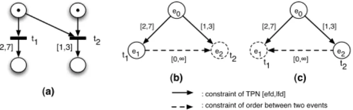
urgency typical to realtime systems. An illustration is given in figure 1(a). Suppose that t1 and t2 are enabled
at the date 0 by the initial marking. t1could not be fired after the date 3 because t2is fired at the latest at this
date. Thus, the effective time domain of a firing could be modified by a conflict (here [2, 3] instead of [2, 7] for t1). t1 t2 [2,7] [1,3] e0 e1 e2 [2,7] [1,3] [0,∞] : constraint of TPN [efd,lfd] : constraint of order between two events
(a) (b) (c) e0 e1 e2 [2,7] [1,3] [0,∞] t1 t1 t2 t2
Fig. 1.Illustration of the strong semantics
The usual semantics of TPN (used in this paper) is initially defined in [14] and is called strong semantics. Another semantics is called weak semantics where there is no obligation to fire a transition before the upper bound lf d of its firing interval [15]. Only the strong semantics allows to model a watchdog in real-time systems. For the representation of all reachable markings in a state graph, the interleaving semantics is expressed
sequence of fireable transitions from the initial marking m0 (m0 σ
→), and θ = (θ1, θ2, ..., θi, ..., θn) the tuple of
the corresponding firing dates. Usually, the firing date θiof ti is relative to the one of the subsequent firing ti−1
(θ1 is relative to the date θ0 = 0). A firing schedule is the pair (σ, θ). A firing schedule (σ, θ) is feasible iff it
exists a sequence σ such as the transitions in the sequence are successively fireable at the corresponding relative dates in θ.
The partial order semantics (used for the branching processes) is more suitable for expressing the concurrency in a behavior (or run) of a Petri net and avoids the systematic interleavings causing the state explosion problem.
3
Temporal assessment on events
A causal net (or process) expresses a behavior of TPN in the partial order semantics. In the interleaving semantics, a date is relative to the previous firing, what is unsuitable for independent firings (i.e. concurrent events) in the partial order semantics. To keep the temporal independence between the concurrent events of the process, a simple way consists in choosing a global time reference like the instant of production of the initial
state. This date matches to a fictitious event e0 and is supposed equal to 0. Thus, an absolute firing date is
associated to each event of the process.
Let exbe an event with λ(ex) = t. According to the weak semantics, its absolute occurrence date denoted
Dx is given by:
Dx= d(t) + max({Dy| ey ∈•(•ex) ∪ {e0}}) (1)
with d(t) ∈ [ef d(t), lf d(t)]. Any event ey ∈ •(•ex) ∪ {e0} will be called an enabling event of ex. The absolute
time domain of ex is the interval [Dxmin, Dxmax] such that Dxmin = ef d(t) + max({Dkmin | ek ∈•(•ex)}) and
Dxmax = lf d(t) + max({Dkmax| ek∈•(•ex)}).
In a general way, the expression 1 remains valid and sufficient in the strong semantics if exis not subjected
to any conflict, the evaluations about enabling events being supposed already known.
In case of conflict, the time domain of an event could become more restrictive because of the strong semantics (as shows the example figure 1), or even, the event is impossible with no valid time domain. For instance, the realtime programs could contain some execution loop where finiteness depends on the time bound of some
repetitive action. In term of unfolding of a TPN, the validness of each underlying event1 in conflict must be
checked. So, a method for the quantitative temporal assessment (such as one used to obtain the canonical form of a firing domain of a state class [21], based on the shortest path algorithm also called Floyd-Warshall algorithm [16, 17]) is needed to know if a valid time domain exists for each event under a conflict.
The time domain of an event ex depends on two kinds of temporal constraints:
– the own constraints of ex due to the delay specification (ef d/lf d) of the transition and the time domains
of the enabling events;
– the vicinity constraints of exdue to the time domains of the events liable to preempt ex, that is the events
in Conf (ex). It is assumed that all the conflict constraints of an event are known before to assess its time
domain. This is reached by sufficiently unfold the net.
About the vicinity constraints of ex, notice that Conf (ex) does not indicate the events that will be really
enabled at the moment of the occurrence of ex, but gives the events can potentially preempt ex.
A process of TPN can be translated into a simple temporal problem (STP) [17] that helps the assessment of time difference between events. A temporal constraint between two events corresponds to a convex interval. The network of the STP can be represented by a directed constraint graph, where nodes represent variables of
events, and an edge between two nodes indicates the interval of the constraint. The absolute date variable Dx
of an event ex is relative to 0, the date of the reference event e0.
Let be aij ≤ Dj− Di≤ bij, the constraint between two events ei and ej. The edge from eito ej (notice that
only one edge could be defined between two nodes) is labeled by the interval [aij, bij] in the constraint graph.
1
The constraint graph is translated into a distance graph that gets the same nodes as the constraint graph, and
an edge ei→ ej labeled by [aij, bij] is split into two edges: an edge ei→ ej labeled by bij, and an edge ej → ei
labeled by −aij. The application of the shortest path algorithm determines the intersection of the intervals of
the possible paths between all pair of events, and tells if the problem is consistent.
For the temporal assessment of an event ei to choose in a conflict, since eipreempts the events in Conf (ei),
an edge ei→ ej(ej ∈ Conf (ei)) labeled by the interval [0, ∞] will express the order constraint. So, the directed
constraint graph of the net figure 1(a) is given figure (b) if e1 is produced, or figure (c) if e2 is produced. The
application of the shortest path algorithm on the resulting distance graph gives D1∈ [2, 3] for (b) and D2∈ [1, 3]
for (c).
For a process of TPN, there exists at least as much paths reaching an event as causes (the enabling events). But, in a constraint graph, multiple causes for an event (expressing an intersection) does not have the same meaning as for TPNs (see the equation 1). Using the method in [17] requires only one enabling event; then, in case of multiple causes, only one effective cause is considered (the last enabling event produced), what means that the other causes are previously produced: a constraint [0, ∞] is defined from each other cause toward the effective cause. All combinations must be considered.
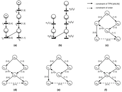
t2 [1,3] t4 t1 t3 t5 [1,3] [3,4] [0,0] [1,1] (a) (b) e2(t2) e4(t4) e1(t1) e3(t3) e5(t5) : constraint of TPN [efd,lfd] : constraint of order (d) (f) e0 e1 e2 e4 e3 e5 [1,3] [3,4] [1,1] [1,3] [0,0] [0,∞] [0,∞] (c) (e) e0 e1 e2 e4 e3 e5 [1,3] [3,4] [1,1] [1,3] [0,0] [0,∞] [0,∞] e0 e1 e2 e4 e3 e5 [1,3] [3,4] [1,1] [1,3] [0,0] [0,∞] [0,∞] e0 e1 e2 e4 e3 e5 [1,3] [3,4] [1,1] [1,3] [0,0] [0,∞] [0,∞]
Fig. 2.Example of unfolding (b) of a net (a) and the temporal assessment (c,d) on e5 (e,f)
An example is given figure 2: the unfolding of a net (a) is given at (b). The two events e5 and e3 are in
conflict and e5has two enabling events e1and e4. When e3is the preempting event in the process {e1, e2, e4, e3},
the temporal assessment gives D3∈ [3, 4] for the first interleaving e4; e1(c), and D3∈ [3, 6] for the second e1; e4
(d). More generally, the (convex) time domain of an event is the union of the valid domains obtained for the
different combinations. So, D3 ∈ [3, 6]. When e5 is the preempting event in the process {e1, e2, e4, e5}, the
temporal assessment gives D5 ∈ [3, 4] for the first interleaving e4; e1 (c), the second interleaving e1; e4 (d) is
inconsistent and so D5∈ [3, 4]. Notice that the conflict-free evaluations with the formulae 1 gives D3∈ [3, 6] and
D5 ∈ [3, 7]; the example shows that it is the event with the smallest Dmax (here e3) that constrains more the
other events in the conflict (here e5) by the means of the order constraint (the arc labeled [0, ∞]). In all, three
where the concurrent events, e1 with e2 and e1 with e4, are interleaved) will give five valid combinations. The
method saves some interleavings, even more since there is a great number of concurrent events.
If a non sequential process is composed of n events, and each event ei gets ni causes, the number of
combi-nations could be exponential (Qni=1ni). Each combination is computed in a polynomial time by the application
of the shortest path algorithm.
It is assumed that the time diverges during a run of a TPN. This implies that any concurrent but temporal
predecessor of an event ex ends up occurring. Thus, the valid assessment on an (effective) event exin a process
also implies that it will necessarily occur.
4
Computing of TPN processes
4.1 Need of conflicts interleaving
In [18] was presented a method allowing to analyze in the weak semantics a behavior of a TPN defined as a scenario (a multiset of transitions). Unlike the unfolding technique that can compute all the alternative behaviors, only one run is considered in the form of a predetermined scenario. Thanks to a temporal labeling of propositions during the proof of a scenario translated in Linear Logic [19], symbolic expressions on firing dates are derived for the analysis. An extension for the strong semantics is made in [13]: it is based on the observation that the symbolic date of a firing in a structural conflict can depend on the order of the resolution of the conflicts. In the next subsection, this paper will formalize the concept of scenario in the context of the unfolding of a TPN.
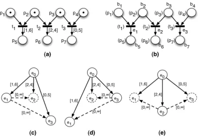
As shows the net figure 3(a), the concurrent firings t1 and t3 form a process; if t1 is fired before t3 (figure
3(c)), the time domains are respectively [1, 4] and [1, 5], but if t3 is fired before t1 (figure 3(d)), the domains
are respectively [0, 4] and [1, 6]. The reason of the difference is that the conflict constraints set depend on the
occurrence of a concurrent event in conflict. In the first case, Conf (e1) = {e2} and Conf (e3) = {}; in the
second case, Conf (e1) = {} and Conf (e3) = {e2}.
Let be e, the event in conflict whose time domain has to be assessed, and the set Bconf(e) =•Conf (e)\(•e ∩
•Conf (e)) containing the preconditions of the events in Conf (e) that are concurrent to e. B
conf(e) decides the
effective constraints Conf (e) applied on e.
Proposition 4.1. The existence of a condition in the set Bconf(e) could be called into question by the occurrence
of a concurrent event to e subject to conflict and done before e.
For instance, in the first case of the previous example, the occurrence of e1 before e3 makes unavailable the
condition b2 in the set Bconf(e3), so e2can not constrain e3.
An easy way to know the concurrent events that decide Bconf(e) is to interleave all the solvings of conflicts
in the process. Thus, according to the position of e in an interleaving, all the concurrent events in conflict (called concurrent choices) occurred before e are known, and so, Conf (e) could be determined as a single set.
To summarize, the relations (≺ and ≀) between the events in a process is not sufficient for the temporal characterization in a single way; there is needed to be enriched by a new relation, a total order relation between the concurrent choices. In a constraint graph, this is translated by an edge between two following concurrent choices labeled by the interval [0, ∞] (see the figures 3 (c) and (d) for the given examples).
Generally, during the process of the unfolding of a net, the concurrent nodes can be known only in a certain order. Thus, the knowledge of the neighboring events in conflict is not certain when producing an event. So, an event in a conflict is not always detectable at the moment it is produced. For the sake of simplicity, any event in a structural conflict of the TPN will be subjected to the interleavings.
4.2 Scenario
Let be N =< N′, ef d, lf d, m0 >, a marked TPN where N′ =< P, T , W >. U nfF =< OF, λF > is the the
unfolding of N′ with O
F =< BF, EF, FF >. < Ci = Bi, Ei, Fi > is a prefix of causal net in OF (Bi ⊂ BF and
[1,6] t1 p1 [2,4] [0,5] t2 t3 p2 p3 p4 (b) (a) e0 e1 e3 [1,6] [0,5] [0,∞] e2 [2,4] [0,∞] e0 e1 e3 [1,6] [0,5] [0,∞] e2 [2,4] [0,∞] (d) (c) (t1) (p1) (t2) (t3) (p2) (p3) (p4) e1 e2 e3 (p5) (p6) (p7) p5 p6 p7 b1 b2 b3 b4 b5 b6 b7 e0 e1 e3 [1,6] [0,5] [0,∞] e2 [2,4] [0,∞] (e)
Fig. 3.Necessity of interleavings in case of conflict
A transition t of N in a structural conflict iff: |(•t)•| > 1. Sconf (Ei) is the set of events in a structural
conflict: Sconf (Ei) = {e ∈ Ei| λF(e) = t , t ∈ T ∧ (•t)• > 1}. Since only events in Sconf (Ei) are interleaved, a
strict order relation ⊆ Sconf (Ei) × Sconf (Ei) is defined. Two events in conflict in U nfF are not necessarily
in a structural conflict. Such a conflict not structural is due to the non safeness of the underlying net. To avoid this problem, the underlying net must also be safe. To ensure safeness when unfolding, it is sufficient to check every time when a new post-condition is created that there is no previous concurrent condition with the same label in P.
In a process of a TPN, an event will be denoted x, and is an extension of a corresponding underlying event e if it exists a feasible firing schedule containing this event.
Let be X , a set of events of a TPN process. Ci is the related causal net if the relation between X and Ei is
a bijection µ : X 7→ Ei.
The causal net Ci with many concurrent choices can allow many interleavings of these choices. A process
of the TPN with an imposed sequence of the choices will be called a scenario. A scenario S of Ci is the set X
respecting a defined strict order relation : S =< X , >.
A scenario is characterized by the set(s) of binary temporal constraints issued from the STP(s) of the process on its events. In the sequel, the temporal information attached to an event e to form an event x of a scenario is not specified. It could be all the binary temporal relations between x and the events that determine or constraint its occurrence, or just the absolute time domain of x.
4.3 Computation of scenarios
All the causal nets can be generated from the initial state M in(OF) by producing the enabled concurrent events
one by one. The first ancestor of all causal nets is the net C0only constituted by the initial conditions M in(OF).
Later, the fictitious event e0 will be considered (by abuse) belonging to C0: E0= {e0}.
The possible extensions of a causal net Ci, denoted P E(Ei), are the set of new events that can be derived
from its maximal concurrent conditions M ax(Ci): P E(Ei) = {e ∈ EF |•e ⊂ M ax(Ci)}.
To extend Ci, an event ei+1 ∈ P E(Ei) is produced and added to Ei, and it is assumed that the condition(s)
e•
i+1 are produced immediately after and added to Bi. Ci+1=< Bi+1, Ei+1, Fi+1>, with Ei+1= Ei∪ {ei+1} and
Bi+1= Bi∪ e•i+1, is a derivative
2
net of the prefix net Ci.
2
The objective is to compute all the scenarios of a time Petri net by ensuring a valid temporal assessment on each produced event in a scenario before constructing its causal successors. The method is based on the rule expressed by the following proposition:
Proposition 4.2. To extend a causal net, the priority is given to the production of the events (and their
post-conditions) free of structural conflict.
Definition 4.2. A causal net Ci is said in a choice state iff: ∀e ∈ P E(Ei), e ∈ Sconf (EF).
Let be Sj =< Xj, j> a scenario of Ci in a choice state, with: µj : Xj 7→ Ei. To each event ei+1 ∈ P E(Ei)
corresponds one derivative net Ci+1 with the derivative scenario Sj+1 =< Xj+1, j+1> such as: Xj+1 =
Xj∪ {xj+1}, µj+1 : Xj+1 7→ Ej+1 (∀x ∈ Xj+1, if x = xj+1 then µj+1(x) = ei+1, else µj+1(x) = µj(x)), and
j+1 = j∪{(e, ei+1) | e ∈ Sconf (Ei)}.
Assumption 41 Any run of the TPN is made of a finite number of events.
This assumption will be relaxed later to take into account a class of systems with infinite runs, without ques-tioning the theorems in the sequel.
From a net Ci, some event ei+1∈ P E(Ei) without structural conflict is produced, and every extension ei+1
matches to a derivative net Ci+1. Since any run is finite, a process of successive extensions from C0will end up
by a derivative net Cn such as no more event without structural conflict is producible. If P E(En) is not empty,
then Cn is in the first choice state.
There is only one derivative net Cn in a first choice state. Indeed, since no choice is made in Cn, there is
no alternative to this execution. The events of P E(En) are the first possible choices in the possible runs of the
underlying net N′. Notice that all the conflict-free events En will necessary occur in the timed extension N ,
even if the time specification could forbid some orderings between concurrent events.
Theorem 4.1. The proposition 4.2 is adequate for identifying all the interleavings of choices in the unfolding
U nfF of N′.
Proof. By induction:
– From the first choice state, all first possible choices are known, and making one of the choices leads to a
distinct scenario.
– Let be the mthchoice state (that means (m − 1) choices have been made previously in the unfolded scenario
and causal net to reach this state). It is assumed that all the possible choices from this state are known, and each choice will be made in a corresponding derivative scenario.
– Let be en, the choice made in the mthstate. After production of en, all the next choices having the causal
predecessor en are found (by applying the rule of the proposition 4.2), and let be the (m + 1)thchoice state
reached when a conflict-free event is no more producible. Any other next possible choice (that is not derived
from en) in this state is a concurrent event of en enabled but not produced from the mth choice state.
Likewise, each choice will be made in a corresponding derivative scenario.
Thus, all possible choices are known from any choice state, and in a next choice state, all the possible choices that are feasible after a previous choice are also known. Then, all the interleavings of choices are known when the corresponding scenarios are completely unfolded.
According to the assumption 41, any choice state is reached in a finite time. Since an interleaving of choices in a causal net corresponds to a scenario of the TPN, the method allows to extract all possible scenarios of the TPN, provided that each choice is submitted to an assessment to ensure that it is not prevented by another event in conflict.
4.4 Method for adequate temporal assessment
A temporal assessment is necessary to know if an event is possible in some feasible firing schedule or in some TPN process. The temporal assessment of a conflict-free event only depends on its own constraints (see the subsection 3). For an event in conflict, the vicinity constraints must be enriched with the informations about the total ordering of the choices, that may impose adding temporal restrictions on the event. An interleaving will be impossible if an event could never respect its temporal order (according to the relation ). With the method presented in this work, the objective is to guarantee that for each event produced in a scenario, a valid temporal assessment is done before producing its successors. This supposes that all temporal constraints due to the interleaving of conflicts and to the conflict constraints are known before the assessment. The proposition 4.2 guarantees that all these constraints are known in a choice state (see the proof of the theorem 4.1).
Let be: a causal net Ci in a choice state, the corresponding scenario Sj, and the next choice xj+1 (with
µj+1(xj+1) = ei+1 ∈ P E(Ei)) in a derivative scenario Sj+1. The extended conflict constraints of the event ei+1
is the set: EConf (ei+1) = {e | e ∈ Sconf (Ei) ∨ e ∈ P E(Ei) ∧ e 6= ei+1} = Conf (ei+1) ∪ {e | e ≀ ei+1, e ∈
Sconf (Ei) ∪ P E(Ei)}. So, the vicinity constraints are extended to the temporal effect of the concurrent choices.
All events in Ei is assumed already getting a valid temporal assessment. The temporal assessment on xj+1
not only depends on the events in ••ei+1, but also depends the ability to pass ei+1 after the past concurrent
choices in Ei and before any other future choice in P E(Ei). The assessment is done by applying the shortest
path algorithm on the resulting STPs. The constraint graphs about the events of the scenario Sj are completed
by the following steps to obtain the scenario Sj+1:
– in relation with an effective cause, define the constraint [ef d, lf d] for ei+1 and the other events in P E(Ei);
– if a past choice is in the local configuration of ei+1, then the temporal order is naturally taken into account;
else (the past choice is concurrent to ei+1), the temporal order is guaranteed by defining a constraint
[0, ∞] from this past choice in Ei to ei+1;
– to express that ei+1 preempts any other choices in P E(Ei), a constraint [0, ∞] is defined from ei+1 to each
other choices in P E(Ei). These constraints guarantee the relation with any future concurrent choice.
The derivative scenario Sj+1 is valid if it exists at least one consistent constraint graph.
For illustrations, the unfolding of the net figure 3(a) gives three scenarios:
– at (c): S1=< X1, 1> with X1= {x1, x2}, µ1(x1) = e1, µ1(x2) = e3, and 1= {(e1, e3)};
– at (d): S2=< X2, 2> with X2= {x3, x4}, µ2(x3) = e3, µ2(x4) = e1, and 2= {(e3, e1)};
– at (e): S3=< X3, 3> with X3= {x5}, µ3(x5) = e2and 3= {}.
Notice that the scenarios S1and S2 get the same causal net, and correspond to the interleavings of the choices
e1 and e3. The unfolding of a TPN (like the example 3(b)) represents all the temporally possible events and
conditions of the unfolding of the underlying net.
5
Cut-off issue
In practice, a system modeled with TPN often expresses behaviors with infinite runs. The purpose is to provide an algorithm to construct a finite unfolding of such TPN, that terminates when all the reachable states are represented, and to generate all prefixes of scenarios contained into the unfolding for permitting quantitative time analyses: in this way, the unfolding is said complete.
For a system with infinite runs, the finite construction of a state class graph [20, 21] is based on the concept of equivalence between state classes. In a state class, the temporal constraints are only relating to the firing that directly leads to this class, and do not cover all the sequence that leads to this class. It is certainly possible to retrieve the temporal profile of a sequence by a treatment on all the classes crossed by this sequence [22], but such a quantitative analysis is based on the interleaving semantics.
The state class graph is finite if and only if the TPN is bounded. Since the boundedness property is undecid-able for TPNs, some sufficient conditions are given [21] to ensure the finiteness of the state class graph. Anyway,
the test of these conditions is based on the enumeration of all the reachable markings, and thus, seems difficult to extend in this context of the unfolding of a TPN where the global markings are not explicitly covered.
The concept of state equivalence is similar to the notion of cut-off in the branching process theory. For
untimed Petri net [7], a configuration is defined as the set of events Ei of a causal net Ci, and M ark(Ei)
represents the reachable marking corresponding to M ax(Ci), that is the marking reached by producing all the
events in Ei. An event e ∈ Ei is a cut-off event if: ∃e′∈ Ei, e′ ≺ e ∧ (M ark([e′]) = M ark([e])) ∧ (λ(e′) = λ(e)).
For an untimed Petri net, a cutoff event determines a local state already reached in the past: this local point of view is tolerable because the time does not restrict possible developments on concurrent events. There could exist many cutoff events in the same unfolding.
In a time Petri net, the cutoff notion needs to be linked to the global state of the scenarios because the local point of view could prevent to see how possible temporal restrictions on concurrent events could determine the future dynamics. During the unfolding of a causal net, concurrent events are produced in an arbitrary order without any consideration on the time, and it is only certain global states that are visited. In this context, a stop condition for a cut-off may concern a global state that is always visited whatever is the order adopted to
produce the events. Only concurrent-free events generate such a state. In a causal net Ci (with ei the latest
event produced as extension), ei is a concurrent-free event if it gets no concurrent event in the past (Ei) or in
the future (P E(Ei)), that is expressed by the following definition:
Definition 5.3. An event ei of a causal net Ci is a concurrent-free event iff: ∀e ∈ Ei, e ∈ [ei] and ∄e ∈
P E(Ei), e ≀ ei.
Only concurrent-free events are candidate to be cutoff because the global states they generates are covered,
whatever is the production order of the events Ei. The first concurrent-free event is the fictitious event e0 that
generates the initial state. A reset state is the global state generates by a concurrent-free event: any event extensible from this state is a newly enabled transition.
A scenario will be stopped when the process of unfolding reaches a reset state already discovered (possibly in another previously computed scenario) with the same corresponding marking. The past state previously discovered is called a return state. The next event, from which the scenario is stopped by the cutoff event, and the event that generates a return state are called a report event. A cutoff event brings back to a return state where the same extensions of runs are possible from its report event. A quantitative analysis can be carried on from the report event on the computed prefix of the unfolding, and every event of a behavior exceeding the prefix can be reported to an event of this prefix.
For a safe TPN, a restriction may be stated to guarantee the finiteness and completeness of the unfolding thanks to the detection of an equivalent return state for any non-terminating run.
Assumption 51 A finite number of events is produced between two consecutive reset states in any infinite run.
This assumption is the relaxation of the assumption 41.
Theorem 5.2. Under the assumption 51, a finite complete prefix exists and is computable for a TPN.
Proof. 1. The system is safe and the set of transitions T and places P are finite. So, there is a finite number of reachable markings, and a finite number of enabled transitions per reachable marking. Consequently, there is a finite number of reset states.
2. An infinite run goes infinitely through at least one reset state since there are a finite number of reset states (item 1) and a finite number of states between two consecutive reset states (assumption ass:finite2). When a reset state is encountered for a second time, the unfolding of the scenario is stopped (cutoff detection). So, a finite prefix is computable for each infinite run.
3. The conflicts determine the nodes of derivation of multiple scenarios. There is a finite number of events per choice state. Consequently, since every scenario gets a finite prefix (item 2), there is a finite number of prefix of scenarios (or terminating scenarios with no cutoff).
4. The unfolding of a TPN results from the finite set of possible events computed in the scenarios. So, this unfolding is finite since there exists a finite number of scenarios (item 3). It is also complete since a cut-off expresses a return to a state from which the same reachable markings and dynamics are feasible.
The theorems and definitions resulting from the assumption 41 remain valid since an infinite run is captured by a finite prefix.
As it was aforementioned, the finiteness of the unfolding of a TPN is undecidable because it is based here on the detection of reachable markings. The fact that the reset states are a subset of the reachable marking makes this problem more difficult than for the state class graph construction.
In spite of the explosive nature of the state class graph, the finiteness of its construction may decide the finiteness of the unfolding. To ensure a finite construction of the unfolding, the solution proposed now and based on the state class graph keeps all the same an interest because allowing a partial order quantitative analysis unlike the method describes in [22]. The theorem given in the sequel is based on the following restricted class of
TPNs: ∀t ∈ T , ∃p ∈ P | p ∈ t•∧ p /∈•t. So, every transition of the TPN gets an exclusively postcondition place.
Theorem 5.3. If every elementary loop of the state class graph contains a firing txand the class C (resp. C′)
with the global marking m (resp. m′) such that: m′ tx
→ m ∧ ∀ty| m
ty
→,•ty⊆ t•
x, then the assumption 51 is always
true.
Proof. The elementary circuits are computable on the state class graph and the reset states are identified in the looped sequence of each circuit. The problem is the identification of the concurrent-free events on the edges between two state classes of the circuit.
The sufficient condition m′ tx
→ m ∧ ∀ty | m
ty
→,•ty ⊆ t•
x makes the class C being a node from that any
transition ty is newly enabled and has tx as the unique enabling event: there is no concurrent event following
the firing tx in a sequence.
It is also necessary to ensure that every predecessor event in a sequence is causal to tx: there is no concurrent
event preceding the firing tx.
How to check this second implicit condition? Assume the existence of some event(s) temporally preceding
the firing tx but concurrent to tx. Since every successor ty of tx gets the unique enabling cause tx, it exists a
predecessor firing tz concurrent with tx but without a successor event. After several loops on the circuit, the
markings do not change. But the firing of tz after many iterations of a circuit will strictly increase the marking
in its next class because tzgets a sink place (an exclusively postcondition place) in which the number of tokens
increases indefinitely after each iteration without never be consumed by some firing. This is a contradiction, so
the assumption of the existence of such a transition tz is false.
Thus, txis a concurrent-free event and the class C corresponds to a reset state. Since the state class graph
is finite, any infinite sequence follows the same (elementary) circuit a least two times, and then crosses a same reset state after a finite number of states or events. So, the assumption 51 is always checked.
6
Quantitative time analyses
The TPN unfolding contains all the temporally possible events (that is the events appearing in some scenario) of the underlying net. A complete prefix of the TPN unfolding covers the overall possible temporal behaviors of the system, and can help to operate some time quantitative analyses.
When the system (or subsystem) is always terminating, the full unfolding allows to directly obtain temporal informations about events. Thus, this work, that takes into account concurrency between events in conflict, is a generalization for an application on modular unfolding [12]; the time domain of an output event (terminating each scenario) is the time interval between an input event and this event, and is provided by the shortest path algorithm. In a general way, the possible delays between any two events can be obtained by the new method.
Another application is the checking the validness of a timing on a firing schedule (with absolute dates attached to the firings) or on a time process [23], even with non terminating systems, with no need to recompute
every time the corresponding causal net of the process as in [23], since this net is contained in the TPN unfolding.
Given a firing schedule (σn, θ), the resulting causal net Cn is identified progressively in the unfolding T U nf by
simulating the sequence σn = t1· ... · ti· ... · tn : from the net Ci−1, the derivative net Ci is obtained by finding
the event ei (λ(ei) = ti) in P E(Ei−1) and by replacing in the B-cut M ax(Ci−1) the preconditions •ei by the
postconditions e•
i to obtain the new B-cut M ax(Ci). Two inequations (validness criteria defined in [23]) are
used to check that θi is a valid time: θi ≥ Ed(ei) + ef d(ti) and ∀ej ∈ P E(Ei−1), Ed(ej) + lf d(λ(ej)), where
Ed(e) = max({θa| ea∈••e ∪ {e0}}) is the enabling date of the event e.
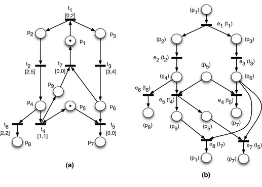
t1 [0,2] (a) t3 [3,4] t2 [2,5] t5 [0,0] t4 [1,1] t6 [2,2] p1 p2 p3 p4 p5 p6 p7 p8 (b) e1 (t1) (p1) p9 t7 [0,0] (p2) (p3) (p4) (p5) (p6) (p8) (p9) (p5) (p7) (p1) e2 (t2) e3 (t3) e6 (t6) e5 (t4) e4 (t5) e8 (t7) (p7) e7 (t5)
Fig. 4.Case study
The unfolding of the TPN figure 4(a) is made with three scenarios 3
:
– Scenario 1: the set of events is {e1, e2, e3, e4, e6} with e4 e6 (no cut-off);
– Scenario 2: the set of events is {e1, e2, e3, e5, e7} with e5 e7 (no cut-off);
– Scenario 3: the set of events is {e1, e2, e3, e5, e8} with e5 e8, and the cut-off is e8 with the report event e0.
The events {e1, ..., e8} and their preconditions and postconditions make up T U nf in figure 4(b).
For instance, if σ1= t1· t2· t3· t4 and θ1= (0, 3, 3, 4), the causal net of the three first firings is made of the
events {e1, e2, e3} with a valid timing; in this state, the last firing t4 (event e5) is invalid because the event e4
also enabled necessarily occurs before at date 3. So, the firing schedule is unfeasible.
Even if a firing schedule or a time process exceeds the unfolding, the analysis could be carried on thanks
to a report event. For instance, let be a firing schedule with σ2 = t1· t2· t4· t3· t7· t1· t3· t2· t5· t6 and
θ2 = (1, 3, 4, 5, 5, 7, 11, 11, 11, 13). When t7 is fired, there is no more possible extensions in T U nf ; since the
prefix of sequence t1· t2· t4· t3· t7 belongs to the third scenario that has the cutoff e8(t7), the checking is
continued from the conditions generated by the report event e0 (here the initial state of T U nf ). The suffix
t1· t3· t2· t5· t6of σ2belongs to the first scenario that has no cutoff event. The timing of the sequence is valid,
3
and there is no more possible extension after firing t6. The existence of a non extensible scenario means that
the system gets a deadlock state or a terminating state.
In [22], a method is presented to characterize one sequence in a state class graph by a timing profile. A third application here is the possibility to depict completely a TPN by a permanent set of quantitative time constraints characterizing all the possible runs of this net. It is based on the possibility to break down a scenario containing concurrent-free events into some parts for an autonomous quantitative time analysis.
Let be a process E of T U nf containing at least one concurrent-free event ek: ∀e ∈ E, e 4 ek∨ ek 4e. Let
be two events ei, ej∈ E such as ei≺ ek and ek ≺ ej. If the time difference between ei and ek (resp. ek and ej)
is denoted by the variable Di,k (resp. Dk,j), then the triangular relation Di,j = Di,k+ Dk,j is proven because
a shortest path from ei to ej passes necessarily through ek. So, ek could be a reference event for ej, instead of
e0, to make the assessment of the time difference with any event ei causal to ek. Thus, the temporal assessment
(see section 3) on any event ej such as ek ≺ ej could have the reference ek with no need to consider any event
ei coming before ek.
Definition 6.4. Let be two consecutive 4
concurrent-free events e1 and e2 (with e1 ≺ e2) in E. The subset
E′ = {e ∈ E | e1 ≺ e ∧ e 4 e2} is a minimal autonomous part of the process E. The event e1∈ E/ ′ is the input
event for E′ and the event e2∈ E′ is the output event for E′.
The set E′ is said minimal because it contains the only one concurrent-free event e
2. It is said autonomous
because a corresponding sub-scenario could be temporally assessed locally; the time difference with any outside
event e ∈ E\E′ may be established by the means of the input event e
1 when e ≺ e1or the output event e2 when
e2≺ e. Notice that e2 could be a cutoff event to map with one report event and e1 could be the reference e0.
An autonomous subprocess E′is said terminating when there is no possible future extension in the unfolding:
if C′ is the corresponding causal net of E′, then P E(E′) = ∅. So, a terminating minimal autonomous subprocess
is a suffix of a terminating process broken down into its minimal autonomous subprocesses. The division of a scenario into some autonomous parts during the TPN unfolding may reduce the cost of temporal assessment because this evaluation is limited to the events of one autonomous part.
To illustrate, the (prefix of) scenarios of the net figure 4(a) gets three concurrent-free events: e1, e7 and e8.
So, the minimal autonomous subprocesses are:
– E1 = {e1} with the input event e0 and the output event e1. E1 is the prefix in each one of the previously
given scenarios;
– E2 = {e2, e3, e4, e6} with the input event e1 and no output event. E2 is terminating and is the suffix of
scenario 1;
– E3= {e2, e3, e5, e7} with the input event e1 and the output event e7. E3is terminating and is the suffix of
scenario 2;
– E4 = {e2, e3, e5, e8} with the input event e1 and the output event e8 related to the report event e0. E4 is
the suffix of scenario 3.
Each one of these subprocesses corresponds to a sub-scenario characterized by a normal form of timing profile, acquired by the application of the shortest path algorithm on the events of this sub-scenario:
– for E1 in the three scenarios: 0 ≤ D0,1≤ 2;
– for E2 with the interleaving e4 e6in scenario 1: 2 ≤ D1,2≤ 5 ∧ 3 ≤ D1,3≤ 4 ∧ 4 ≤ D1,6≤ 7 ∧ − 2 ≤
D2,3≤ 2 ∧ 2 ≤ D2,6≤ 2 ∧ 0 ≤ D5,6≤ 4 ∧ D3,4= 0;
– for E3 with the interleaving e5 e7 in scenario 2: (2 ≤ D1,2≤ 3 ∧ 3 ≤ D1,3≤ 4 ∧ 3 ≤ D1,5≤ 4 ∧ 1 ≤
D2,3≤ 2 ∧ D2,5= 1 ∧ 0 ≤ D5,3≤ 1 ∧ D3,7= 0)
W
(2 ≤ D1,2≤ 5 ∧ 3 ≤ D1,3≤ 4 ∧ 3 ≤ D1,5 ≤
6 ∧ − 2 ≤ D2,3≤ 1 ∧ D2,5= 1 ∧ 0 ≤ D5,3≤ 3 ∧ D5,7= 0);
4
e1 and e2(e1≺ e2 and e1, e2∈ E) are consecutive concurrent-free events iff ∀e ∈ E such as e1≺ e ≺ e2, the event e is
– for E4 with the interleaving e5 e8 in scenario 3: (2 ≤ D1,2≤ 3 ∧ 3 ≤ D1,3≤ 4 ∧ 3 ≤ D1,5≤ 4 ∧ 1 ≤
D2,3≤ 2 ∧ D2,5= 1 ∧ 0 ≤ D5,3≤ 1 ∧ D3,8= 0) W (2 ≤ D1,2≤ 5 ∧ 3 ≤ D1,3≤ 4 ∧ 3 ≤ D1,5 ≤
6 ∧ − 2 ≤ D2,3≤ 1 ∧ D2,5= 1 ∧ 0 ≤ D5,3≤ 3 ∧ D5,8= 0).
A timing profile could be extract from these constraints about any process of the TPN. The first step is to identify the minimal autonomous subprocesses composing this process by the simulation of T U nf . When a process exceeds T U nf , an event of the exceeding suffix may be reported to a mapping event e of T U nf , and
the first event may be labeled by e′, e′′, ...en, according to the number of instances of the equivalent events
in the process. Then, the timing profile is the union of the normal forms of the constraints related to this
subprocesses. For instance, let be a process E = {e1, e2, e3, e5, e8, e′1, e′2, e′3}. In order, the subprocesses are:
Ea= {e1}, Eb= {e2, e3, e5, e8= e′0} and Ec = {e′1} and Ed= {e′2, e′3}. Ea, Eb and Ec is identified respectively
with E1, E4and E1. The suffix Edis included in each of the subprocesses E2, E3and E4but their timing profiles
may not be considered just as there are. The corresponding timing profile must take into account the fact that
the events in Edpreempts any concurrent in P E(E) = P E(Ed). In this example, there is no concurrent for the
events in Ed; but in the general case, the temporal assessment must be made for a suffix not identifiable with
some pre-computed subprocess, by taking into account the preemption of possible concurrent events in P E(E). To conclude, the process E is characterized by the following timing profile obtained by the conjunction of the ones of the subprocesses:
(0 ≤ D0,1≤ 2) V ((2 ≤ D1,2≤ 3 ∧ 3 ≤ D1,3≤ 4 ∧ 3 ≤ D1,5≤ 4 ∧ 1 ≤ D2,3≤ 2 ∧ D2,5= 1 ∧ 0 ≤ D5,3≤
1 ∧ D3,8= 0) ∨ (2 ≤ D1,2≤ 5 ∧ 3 ≤ D1,3≤ 4 ∧ 3 ≤ D1,5≤ 6 ∧ − 2 ≤ D2,3≤ 1 ∧ D2,5= 1 ∧ 0 ≤
D5,3≤ 3 ∧ D5,8= 0)) V (0 ≤ D0′,1′ ≤ 2)
V
(2 ≤ D1′,2′ ≤ 5 ∧ 3 ≤ D1′,3′ ≤ 4 ∧ − 2 ≤ D2′,3′ ≤ 2)
When one is interested to the time difference between two events in the process and not in the same sub-scenario, the triangular relation must be used by using the middle input or output events between these events.
For instance, between e2and e′2, there is the references e8and e′1, so D2,2′ = D2,8+ D0′,1′+ D1′,2′. The variable
D2,8= D2,3gets two possible domains (1 ≤ D2,8≤ 2 ∨ − 2 ≤ D2,8≤ 1). Thus, 3 ≤ D2,2′ ≤ 9 ∨ 3 ≤ D2,2′ ≤ 8,
that implies D2,2′ ∈ [3, 9] (the occurrence periods of the event e2 in an infinite run).
More complex analyses may be carry out from the timing profiles of a TPN unfolding, such as the possible delays between two states, knowing that the difference between the death date and the birth date of markings can be expressed as time difference between some corresponding events.
7
Conclusion
This work shows that the unfolding of a time Petri net requires some interleaving of conflicting events to assess the temporal possibility of the events of the underlying net unfolding. The generated complete finite prefix contains all the possible events of the system (modulo the dynamics from the return states). When the unfolding is finite, a prefix of scenario defines a permanent quantitative temporal relation between the events that form it. The interest is to get a complete and permanent database (T U nf and the timing profiles about the subprocesses of the TPN unfolding) for an immediate temporal analysis (made in a polynomial time) like the checking of a time process or a firing schedule [23], the assessment of the time domain between two events or states, or the timing profile of a process. Contrary to the state class graph construction, the method is not based on the systematic interleaving of the concurrent events, that is the cause of the combinatory explosion when analyzing a complex system with a lot of parallelisms.
The restriction to have a point of synchronization (the concurrent-free events and the return states) after a finite number of actions is not unrealistic for a practical modeling: the modeler may render in the structure of the TPN the synchronization between concurrent events, and may not let the implicit orderings due to the timings settle the synchronizations.
This work imposes that the underlying net to be also safe. A perspective is to remove this restriction. An idea may be to reiterate (partially) the assessment on a scenario when, in the course of the unfolding, several
events in conflict get the same transition in the TPN. Indeed, such a conflict expresses a non-safeness of one preset place of these events, and the temporal reassessment will show that only one of these events is possible if the TPN is safe. Such an approach obviously implies more algorithmic complexity for the method.
References
1. Merlin, P.M.: A Study of the Recoverability of Computing Systems. PhD thesis, Department of Information and Computer Science, University of California (1974)
2. Berthomieu, B., Diaz, M.: Modeling and verification of time dependent systems using time petri nets. IEEE Trans. Softw. Eng. 17(3) (1991) 259–273
3. Berthomieu, B., Vernadat, F.: State class constructions for branching analysis of time petri nets. In: TACAS. (2003) 442–457
4. Yoneda, T., Ryuba, H.: Ctl model checking of time petri nets using geometric regions. IEICE Trans. E81-D(3) (1998) 297–396
5. Sloan, R., Buy, U.: Reduction rules for time petri nets. Acta Informatica 33 (1996) pp 687–706
6. Bucci, G., Vicario, E.: Compositional validation of time-critical systems using communicating time petri nets. IEEE Trans. Softw. Eng. 21(12) (1995) 969–992
7. Esparza, J., R¨omer, S., Vogler, W.: An improvement of mcmillan’s unfolding algorithm. TACAS 1(1055) (1996) 8. McMillan, K.L.: Using unfolding to avoid the state explosion problem in the verification of asynchronous circuits.
In: Proc. Fourth Workshop on Computer-Aided Verification. Volume 663., Montreal, Canada, Springer-Verlag (june 1992) pp 164–177
9. Engelfriet, J.: Branching processes of petri nets. Acta Informatica 28(6) (june 1991) pp 575– 591
10. Semenov, A., Yakovlev, A.: Verification of asynchronous circuits using time petri net unfolding. In: DAC ’96: Proceedings of the 33rd annual conference on Design automation, New York, NY, USA, ACM (1996) 59–62 11. Chatain, T., Jard, C.: Complete finite prefixes of symbolic unfoldings of safe time petri nets. Springer-Verlag 4024
(2006) pp 125–145
12. Sogbohossou, M., Delfieu, D.: Temporal reduction in time petri net. In: IDT 2008, Monastir, Tunisia (December 2008)
13. Delfieu, D., Sogbohossou, M., Traonouez, L.M., Revol, S.: Parameterized study of a time petri net. In: CITSA 2007, Orlando, Florida, USA (July 2007)
14. Merlin, P.M., Faber, D.J.: Recoverability of communication protocol - implications of theoretical study. IEEE Transactions on Communications COM24 (September 1976) pp 1036–1043
15. Cerone, A., Maggiolo-Schettini, A.: Time-based expressivity of time petri nets for system specification. Theoretical Computer Science 216(1-2) (1999) 1 – 53
16. Cormen, T.H., Leiserson, C.E., Rivest, R.L., Stein, C.: Introduction to Algorithms, Second Edition. The MIT Press and McGraw-Hill Book Company (2001)
17. Dechter, R., Meiri, I., Pearl, J.: Temporal constraint networks. Artif. Intell. 49(1-3) (1991) 61–95
18. Pradin-Ch´ezalviel, B., Valette, R., K¨unzle, L.A.: Scenario durations characterization of t-timed petri nets using linear logic”. In: PNPM’99, 8th International Workshop on Petri Nets and Performance Models, Zaragoza, Spain (1999) 208–217
19. Girard, J.Y.: Linear logic. Theoretical Computer Science 50 (1987) 1–102
20. Berthomieu, B., Menasche, M.: An enumerative approach for analyzing time petri nets. In: IFIP Congress. (1983) 41–46
21. Berthomieu, B., Diaz, M.: Modeling and verification of time dependent systems using time petri nets. IEEE Trans. Software Eng. 17(3) (1991) 259–273
22. Vicario, E.: Static analysis and dynamic steering of time-dependent systems. IEEE Trans. Softw. Eng. 27(8) (2001) 728–748