A Generalisation of the Mixture Decomposition Problem in the Symbolic Data Analysis Framework

A GENERALISATION OF THE MIXTURE DECOMPOSITION PROBLEM IN

THE SYMBOLIC DATA ANALYSIS FRAMEWORK

E. Diday 23/4/2001

Summary

In Symbolic Data Analysis, more complex units can be considered like "concepts" (as towns, insurance companies, species of animals). A concept can be characterized by an "extent" defined by a class of standard units called "individuals" (as a sample of inhabitant of a town, a sample of insurance companies, a sample of animals of a given species). These classes can be described by a distribution associated to each variable, summarizing in that way huge sets of data. Therefore, here we are interested by the case where each unit representing a "concept" is described by a vector of p distributions associated to p variables. Our aim is to find simultaneously a "good" partition of these units and a model using "copulas" associated to each class of this partition. Different copulas models are recalled where the case of Markov process and Brownian motion are considered. The mixture decomposition problem is settled in this general case. It extends the standard mixture decomposition problem to the case where each unit is described by a vector of distributions instead as usual, by a vector of unique (categorical or numerical) values. Several generalization of standard algorithms are suggested. One of them is illustrated by a simple example. All these results are first considered in the case of a unique variable and then extended to the case of a vector of p variables by using a top-down binary tree approach. Finally, the case of infinite joint and copulas is considered.

Key-words: Mixture decomposition, Symbolic Data Analysis, Data Mining, Clustering,

Partitioning

1. Introduction

In a symbolic data table, a cell can contain, a distribution (Schweitzer (1984) says that "distributions are the number of the future"!), or intervals, or several values linked by a taxonomy and logical rules, etc.. The need to extend standard data analysis methods (exploratory, clustering, factorial analysis, discrimination,...) to symbolic data table is increasing in order to get more accurate information and summarise extensive data sets by the description of the underlying concepts contained in Data Bases (as towns or socio-economic groups) considered as new kinds of units.

The idea of operating with distribution functions as data is already explicit in Mengers (1949, 1970) writings and applied in clustering by Janowitz and Schweitzer (1989). We are here interested to extend the mixture decomposition problem (as defined for instance in Dempster and al (1977)) to the case where the units are described by distributions.

Here a "variable" is considered to be a mapping from a set of units Ω in a set of distributions. We consider a data table of N rows and p column where each row is associated to a unit belonging in the set Ω and each column is defined by a variable such that the cell of this data table, associated to a given unit and a given variable is a distribution. This set of given initial distributions is called the "distribution base".

We consider first the case of a unique variable "Y" with domain Y ID called description set. We

denote X i the random variable associated to the ith unit (or "individual") and F i its associated

distribution defined by : F i (t) = Pr (X i ≤ t). The distribution base is now reduced to the set

First we define a "point-distribution of distributions" associated to the given variable Y at a point T n by:

G T n (x) = Pr ({F i ∈ F / F i (T n) ≤ x } ) = card({F i ∈ F / F i (T n) ≤ x })/N, where

x ∈ [-∞, +∞ ]. For instance, if x is the median (i.e. x = 1/2) , G T n (x) is the percentage of units

whose probability of taking a value less then T n is less then 1/2.

We define a "k-point joint distribution of distributions" by:

H T1,…,T k (x1,..., x k) = Pr ({F i∈ F / F i (T1) ≤ x1} ∧.... ∧{ F i∈ F / F i (T k) ≤ x k}).

In the following, we suppose that T i is increasing with i and Min {F i (T1)/ F i ∈ F } > 0. Also, in

order to simplify notations, sometimes when there is no ambiguity, H T1,…,T k (x1,..., x k) is replaced

by H (x1,..., x k).

Proposition 1

. G T n is a distribution.

. H T1,…,T k is a k-dimensional joint distribution function with margin G T 1 ,..., G T k

Proof: this results from the definition of a distribution function and a n-dimensional distribution function as G T n is not decreasing and G T n (-∞) = 0, G T n (∞) = 1. Also, H T1,…,T k is n-increasing

and H T1,…,T k (x1,..., x k) = 0 for all X = (x1 ,..., x k) in IR k such that x1 = 0 for at least one i ∈

{1,...,k} . This comes from the fact that {F i (Ti)/ F i∈ F } > 0 as the Fi the T i are increasing and T1

is chosen such that: Min {F i (T1)/ F i ∈ F } > 0. It is also easy to see that H T1,…,T k (∞,..., ∞) = 1 as

H T1,…,T k (1,..., 1) = 1 and H T1,…,T k is increasing.

Definition of a k-copula ( Schweizer and Sklar (1983), Nelsen (1998)):

A k-copula is a function C from [0, 1]k to [0, 1] with the following properties: 1. For every u in [0, 1]n , C(u) = 0 if at least one coordinate of u is 0

2. If all coordinate of u are 1 except u* then C(u) = u*

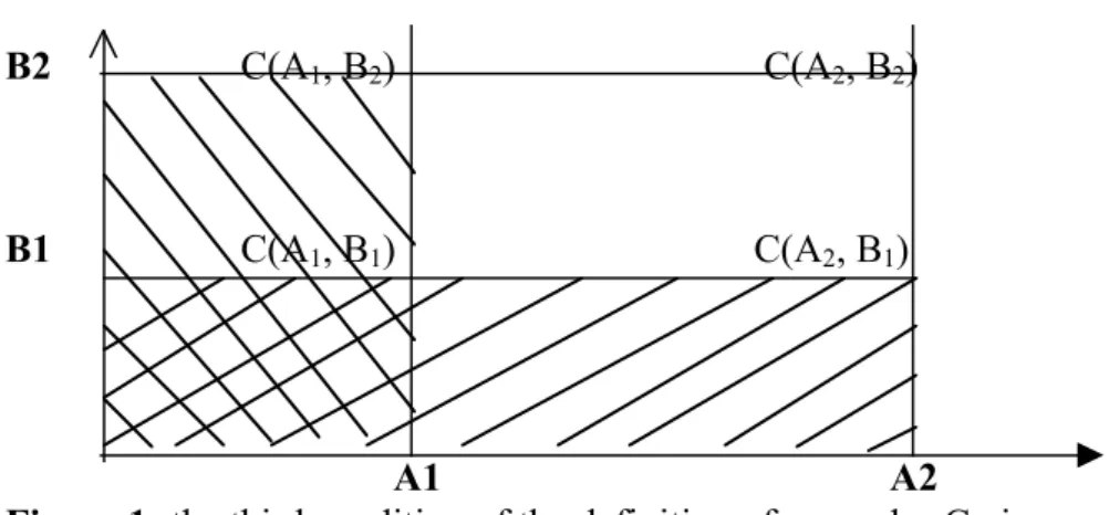
3. The number assigned by C to each hyper-cube [a1, a2] x [b1, b2] x…x [z k , z k] is non negative.

For example, in two dimensions (k = 2), the third condition gives: C(a2, b2)- C(a2, b1)- C(a1, b2)+ C(a1, b1) ≥ 0. See figure 1:

or a*(w, η) = [Y(w) R(η) C(G* T)].

B2 C(A1, B2) C(A2, B2)

B1 C(A1, B1) C(A2, B1)

A1 A2

Figure 1: the third condition of the definition of a copulas C gives:

(1/2) (1/2) (1/2) (1/2) (1/ 2) 1 (0) 1/2 (0) 0 (0)

V

There exist a k-copula C such that for all X = (x1 ,..., x k) ∈ [-∞, +∞ ] k :

H T1,…,T k (x1,...,x k) = C (G T 1 (x1),..., G T k (x k)). Moreover, C is uniquely determined on

Ran G T 1 x...x Ran G T k .

Proof: this results directly from Sklar theorem and proposition 1.

Parametric families of copulas

The most simple copulas denoted M, W and Π are M(u, v) = min(u, v), Π(u, v) = u v and

W(u, v) = max(u+v-1,0). These copulas are special cases of some parametric families of copulas as the followings:

Cb(u,v) = max([u-b + v-b -1]-1/b, 0) discussed by Clayton (1978) has the following special cases:

C-1 = W, C0 = Π, C∞ = M.

Frank (1979) has defined Cb(u,v) = -1/b ln (1+(e-bu-1)(e-bv-1)/(e-b-1)) has the following special

cases: C-∞ = W, C0 = Π, C ∞ = M. Many other families are defined in Nelsen (1998).

In case of a Markov process XT (of distribution GT for instance) we have a transition formulas:

Cst = Csu*Cut where the product * is defined by: (C1*C2) (u,v) = ∫01 ∂C1(u,t)/∂u . ∂C2(t,v)/∂v dt. It is

easy to verify that Π*C= C*Π , M*C = C*M = C and W*W = M. If the transition probability satisfies a standard Brownian motion we have: Cst(u,v) = ∫0u ϕ(√(t ) ϕ-1(v) - √(s) ϕ-1(w)/√(t-s)) dw

where ϕ denote the standard normal distribution function. For more details on the links between Markov processes and copulas , see Darsow , Nguyen, Olsen (1992).

Example: the distribution base (see figure 2) is reduced to two distributions F1 and F2.

F2 x3 x2 F1 x1 x0 T1 T2 T Figure 2: The distribution base is reduced to F1 and F2.

Figure 3: The copulas C(u, v), for instance C(0, 1) = 0, C(1,1/2) = 1/2.

(0) (0) (0)

U

For instance:

G T1 (x1) = Pr({F i ∈ F / F i (T 1) ≤ x 1 } ) = 1

G T2 (x2) = Pr({F i∈ F / F i (T 2) ≤ x 2 } ) = 1/2

H T1,T2 (x1 , x2) = C(G T1 (x1) , G T2 (x2)) = C(1,1/2) = 1/2

From all calculation of C(u, v ), (see figure 3), it results that C = Min.

Example

The space is partitioned in cubes. A distribution of humidity is associated to each cube: F i (t) = Pr

(X i ≤ t) where X i (w) is the humidity at a point w which belongs in the cube i. Hence, the

distribution base is the set of all their associated distributions and F i (t) is the proportion of points

in the cube which humidity is lower than t.

G T n (x) is the proportion of F i such that F i (T n) ≤ x . For instance, if x is a quartile (i.e. x = 1/4) ,

G T n (x) is the percentage of cubes whose probability of taking a humidity lower than T n is less

than 1/4.

If for any x, Gt1(x) = 0 and Gt2(x) = 1 , then this means that the humidity of the cube varies between

t1 and t2.

H T1,T2(x1,x2) = C(G T 1 ( x1), G T 2 ( x2)) is the proportion of cubes which humidity distribution is

lower than x1 and x2 respectively at T1 and T2 (i.e. the proportion of cube distributions which have

a probability of humidity less than x1 at T1 and less than x2 at T2).

Proposition 3

If each point distribution G T 1 ,..., G T k converges, when the size of the distribution base F grows to

infinity, then the k-dimensional joint distribution function H with margin G T 1 ,..., G T k converges.

Proof

This come from the fact that a copula is continuous in its horizontal, vertical and diagonal section (see corollary 2.2.6 in Nelsen (1998)).

2. Symbolic objects associated to a distribution base

A concept is defined by an intent (its characteristic properties, also called its "description") and an extent (the units which "satisfy" these properties). Here, each unit is described by a set of distribution. Together the units define the distributions base and are supposed to satisfy the properties of a given concept. For instance, the units are towns described by socio-economic distributions (as the age or wages distribution of their inhabitant) and the concept is the region containing these towns. More formally, if C is a region, Extent( C ) is the set of towns of this region Intent( C ) = dC is a description of the region. A symbolic object (see Diday (1998) or Bock, Diday

(2000) for more details) is a model for a concept C, it is defined by a triplet s = (a, R, dC) where

here

- dC is the k-point joint distribution of distributions of the distribution base: H T1,…,T k.

- R is a binary relation between descriptions such that the value [d'Rd] ∈ [0,1] measures the degree to which d' is in relation with d (see Bandemer and Nather (1992)).

- " a " measures the "fit" between a unit "w" and the concept C. It is a mapping from Ω into [0,1] such that a(w) = [Y(w) R dC] where Y(w) is the k-point joint distribution of distributions of a

distribution base reduced to Y(w).

The fit between w and C can be measured by different ways, for instance, by the "density of distributions" around Y(w) among the set of descriptions { Y(w') / w' ∈ Extent( C ) }. In this context, the "density" can be defined in two ways in using, first an approximation of the derivative of the copula (see hereunder 2.1), second the derivative of the copula , when it exists! (see 2.2). The fit between w and C can also be measured by comparing the k-point joint distribution of

distributions associated to the unit "w" and to the concept C (see 2.3). In order to simplify, we consider the case k =2 where each unit is described by only two distributions. It is then easy to extend this case to a multivariate copula by using the H-volume (defined in Nelsen (1998), p. 36).

2.1 Fit between a unit and a concept by using an approximation of the density

We define a symbolic object s = (a, R(η), d) such that: a(w, η ) = [Y(w) R(η) Cs

(G T 1 , G T 2 )] ∈ IR+ which measures the "fit" between a distribution

L = Y(w) and the copula Cs (GT 1 , G T 2 ) = H T 1, T 2 associated to the distribution base F.

With xi = L(T i) (the value of the distribution L, at the point T i) , R(η), with η = (ε1, ε1) is defined

by : L R(η)Cs

(G T 1 , G T 2) = (Cs(G T 1 (x1+ε1), G T 2 (x2+ε2))- Cs(G T 1 (x1+ε1), G T 2 (x2- ε2))- Cs (G T 1

(x1- ε1)),G T 2 (x2+ε2)) + Cs (G T 1 (x1- ε1)), G T 2 (x2- ε2))).

Hence, a(w, η) = [Y(w) R(η)Cs

(G T 1, G T 2)] with xi = Y(Ti). Notice that due to proposition 1, G T 1

and G T 2 are increasing, so we have G T i (x i +ε i) ≥ G T i (x i -ε i).

Proposition 4

We have a(w, η) = [Y(w) R(η) C(G T 1 , G T 2 )]∈ [0,1].

Proof: This can be proved in the following way:

a(w, η) = (H(x1+ε1, x2+ε2)- H(x1+ε1, x2- ε2)- H(x1- ε1, x2+ε2) +H(x1-ε1, x2-ε2)).

a(w, η) = (Pr ({F i ∈ F / F i (T1) ≤ x1+ε1}∩{ F i ∈ F / F i (T 2) ≤ x2+ε2})- Pr ({F i ∈ F / F i (T1) ≤

x1+ε1}∩{ F i ∈ F / F i (T 2) ≤ x2-ε2}) - Pr ({F i ∈ F / F i (T1) ≤ x1-ε1}∩{ F i ∈ F / F i (T 2) ≤ x2+ε2})+

Pr ({F i ∈ F / F i (T1) ≤ x1-ε1}∩{ F i ∈ F / F i (T 2) ≤ x2-ε2})) . Finally:

a(w, η) = Pr ({F i ∈ F / x1-ε1 ≤ F i (T1) ≤ x1+ε1}∧{ F i ∈ F / x2-ε2 ≤ F i (T 2)) ≤ x2+ε2}) ∈ [0,1].

2.2 Fit between a unit and a concept by using the derivative of a copula

Let G T = (G T 1 , G T 2) and H T1,…,T k = C(G T). When the derivative of G and of the copula C exist,

we can calculate the derivative of a k-point joint distribution of distributions, in the following way. The density function h associated to the distribution of distributions H, is the derivative of C(G T) at

X = (x1, x2). It is given by:

h(X) = H'T1,T2 (X) = ∂2 HT1,T2 (x1, x2) / ∂ x1∂ x 2 =∂2 C(G T1 (x1), G T2 (x2)) / ∂ x1∂ x 2

h(X) = ∂/ ∂ x1 .∂ G T (x2) / ∂ x 2 ∂ 2C(G T1 (x1), G T 2 (x2)) / ∂u2

h(X) = (∂ G T1 (x1) / ∂ x1) . (∂ G T 2 (x2) / ∂ x 2 ). (∂ 2C(G T (x1), G T (x2)) / ∂u1 ∂u2)

h(X) = G T '(X) C'(G T (X) ) where C'(u1 , u 2 )= ∂ 2C(u1 , u 2 ) / ∂u1 ∂u 2 and

G T ' (x1, x2) = ∂ G T 1 (x1) / ∂ x1 . ∂ G T2 (x2) / ∂ x 2

From the proposition 4 it results:

Proposition 5

When the derivative of G and of the copula C exist, when η→ 0,

a(w, η) = [Y(w) R(η) C(G T 1 , G T 2 )] → a(w,0) = h(L(T1), L(T2)) ∈ [0,1] where Y(w) = L.

Proof

This results from the definition of a(w, η) which converges by definition of a derivative towards the derivative h of H when η→ 0. Moreover, as from the proposition 4, a(w, η) ∈ [0,1], we have h(L(T1), L(T2)) ∈ [0,1].

We call H T1,…,T k, w the k-points joint distribution of distributions associated to the distribution

base F* = { Y(w) } reduced to the single distribution Y(w) denoted F w. In this case, we have the

following result:

Proposition 6

The k-copula C associated to the k-points joint distribution of distributions satisfies the following properties: i) its domain is the set {0, 1}, ii) C = Min or C = ∏.

Proof:

By definition of a "k-point joint distribution of distributions":

H T1,…,T k, w (x1,..., x k) = Pr ({F w (T1) ≤ x1} ∧.... ∧{ F w (T k) ≤ x k}) which is equal to 1 if ∀ i we

have F w (T i) ≤ x i and it is equal to 0 if ∃ i such that F w (T i) > x i . In other words,

H T1,…,T k, w (x1,..., x k) is equal to 1 if ∀ i G T i (xi) = 1 and is equal to 0 if ∃ i such that G T i (xi) = 0.

It results that H T1,…,T k,w (x1,...,x k) = C (G T 1 (x1),..., G T k (x k)) belongs to {0, 1} and moreover the

copula C is the product or the min which leads in this special case to the same result.

Let G T = (G T 1 ,…, G T k) and H(Y) = H T1,…,T k, w . We define the following symbolic object

associated to the distribution base F* and F by:

s = (a, R, C(G T)) with a(w) = [H(Y) R C(G T) ] = [H T1,…,T k, w R C(G T) ] where R measures the

degree to which the k-points (T1, …,Tk) joint distribution of distributions H T1,…,T k, w associated to

the unit w is in relation with the k-points (T1,…,Tk) joint distribution of distributions associated to

the distribution base F associated to a concept. Notice that the R measure can be chosen among standard dissimilarities between distributions function extended to joint distributions function (as Paul Levy, Hellinger, Kullback-Leibler, see Tassy, Legait (1990) for a review).

2.4 Partitioning algorithms and criteria to optimize

The quality on a subset A of Ω of the copula model C when the model of G is chosen can be given by: Q(C,G) = ∏w∈Ω a(w) or Q(C,G) = Min w∈Ω a(w) or Q(C,G) = (∑w∈Ω a(w))/ N to be maximised.

Hence, when we look for a partitioning, the criteria Q has to be maximised for each class.

2.5 The choice of Tj

As we are looking for a partition of the set of distributions, it is sure that a given Tj is bad if all the distribution F i of the base F take the same value at Tj. Also Ti is a bad choice if all the F i (Tj) are

uniformly distributed in [0, 1] . In fact we can say that a Tj is good if distinct classes of values exist among the set of values: { F i (Tj)/ i = 1, N}. In Jain and Dubes (1988) several methods are

proposed in order to reveal clustering tendency. Here we are in the special case were we look for such tendency among a set of points belonging in the interval [0, 1] .

We suggest a method based on the number of triangles whose vertices are points of [0, 1] and where closest sides are larger (resp. smaller) than the remaining side and denoted A (resp. B). We define the hypotheses H° that there is no clustering tendency, by the distribution of a random variable X° which associates to N points randomly distributed in the interval [0, 1] and denoted u, the value X° (u) = A- B / C3N = 6(A-B)/ n(n-1)(n-2) which belongs in [-1, 1]. The greater is X° (u)

the higher is the clustering tendency. We calculate the number of triangles whose vertices are points of U = { F i (Tj)/ i = 1, N} for which the two closest sides are larger (resp. smaller) than the

remaining side and denoted A(U) (resp. B(U)). Having the distribution of X°, the value A(U) -B(U) / C3N can reject or accept the null hypotheses at a given threshold.

3.1 The mixture decomposition problem

The problem can be settled in the following way:

Given k, find a partition P = (P 1,..., P k) of F and the value of k parameters (α1,..., α k), such that

each class P i be considered as a sub-sample which follows the k-dimensional joint distribution

function H i (., α i):

H(X) = ∑i=1,k p i H i (X,α i) where p k ∈ [0,1] and ∑i=1,k p i =1.

In order to solve this problem we can settle it in term of mixture decomposition of density functions, by setting in case of H derivability: h (X) = H'(X) and h i (X, α) = H' i (X, αk). Then the

mixture decomposition problem becomes: given k, find a partition P = (P 1,...,P k) of F and the value

of k parameters (α1,..., α k), such that each class P i be considered as a sub-sample which follows

the k-dimensional joint distribution function h i (.,α i): h(X) = ∑i=1,k p i h i (X, α i). The parameters

α i = (d i, b i) depends on the parameters of a chosen copulas family model (for instance, the Frank

family, see 2.5) denoted b i and on the parameters of a chosen distribution family model denoted d i

(defined on [0,1] like a Dirichlet or Multinomial distribution).

In order to approximate the density function h i (X, α k) or to calculate it, we can use the two ways

presented in section 2. In the first case (see 2.1), which can be also used in case of not derivability of H we settle:

h i (X, αi,η i) = a i (w, η i ) = [Y(w) R(ηi) C i ((GiT 1 (.,d i1), GiT 2 (.,d i2) ), b i )] where X= Y(w),

α i = (d i, b i) with d i = (d i1, d i2) and η i = (ε1i, ε2i). Hence, the mixture decomposition model can be

settled in the following way: h(X) = ∑i=1,k p i h (X, αi, η i).

In the second case (see 2.2), where H, C and G are supposed derivable, we settle: h i (X, αi ) = C i ' (Gi (X, d i ), b i ) with α i = (d i, b i) and

C i ' (Gi (X, d i ), b i ) = ∑i=1,k p i Gi'(X, d i) C i '(G(X, d i), b i ) where

C i ' = ∂ C i / ∂u1 ∂u2 and Gi' = ∂ Gi T 1/ ∂ x1 ∂GiT 2 /∂ x 2.

In the following, we denote β i = (αi,η i) in the first case and β i = αi in the second case . Hence, the

general decomposition model can be expressed in the following way: h(X) = ∑i=1,k p i h (X, β i) .

3.2 The symbolic mixture decomposition problem and four algorithms for solving it:

Given the models associated to G and C, the decomposition can be obtained by maximizing alternatively (Diday et al 1974) a criterion. With L = Y(w), xi = L(T i) and X = (x1, x2) this criterion

can be, the likelihood :

v(X, β) = Πi=1,k p i Π w∈P i h i (X, β i)) where β = (β1,..., β k) are the parameters of the densities h i ,

the log likelihood:

V(X, β) = ∑i=1,k ∑ w∈P i Log (p i h i (X, β i)). Or any measure of the fit between the sample and the

distributions of the mixture decomposition as for instance:

Z(X, β) = ∑i=1,k p i∑w∈P i h i (X, β i)) which will be used in the following example given in 4.4.

We suggest the four following algorithms based on two steps of "maximisation" and "representation" in the framework of the so called "Nuées dynamique" or "dynamical clustering" method (Diday (1971), Diday and al (1979) where here the representation step is an estimation of the parameters of a copula model :

Algorithm 1:

Input: a set of units described by distributions and a number of classes.

Output: a partition and a copula model C i for each class and optionally a distribution G i for each

class at each T i.

This algorithm is defined in two steps of representation and allocation Diday, Ok, Schroeder (1974):

1 . Representation: g(P 1,...,P k) = (β1,..., β k) by finding the parameters (β1,..., β k) which

maximise the chosen criterion (for instance v, V or Z)

2. Maximisation: f (β1,..., β k) = (P 1,..., P k) by finding the partition (P 1,..., P k) where Pi is the set

of distributions:

Pi = {X / p i h i (X, β i) ≥ p m h m (X, β m)) with i < m in case of equality}.

When the criterion are bounded (which is the case of v, V, Z), it is easy to show that this algorithm converges as it increases the criterion at each step.

There are several variants for the choice of pI : pi = card Pi/ N at the last step, or at each step , see

for instance, Celeux, Govaert (1993).

In the first case (defined in 2.1) where η i = (ε1i, ε2i), εi = Min (ε1i, ε2i) is increased until

Max i a i (w, α i ) becomes different from all (or a given number) of a j (w, α j ).

Algorithm 2: SYEM

Input: a set of units described by distributions and a given number of classes.

Output: K copula model C i and optionally k associated distributions G i for each class at each T i.

This algorithm is based on the two steps of the EM algorithm (Dempster, Laird, Rubin (1977)) : We start from an initial solution at step n = 0: (p0l , β0l) for l = 1,k and then, at step n we have :

Estimation: for l = 1,k and any w∈Ω , tn

l (X) = pn l h l (X, βn l) / ∑w_∈Ω pn l h i (X, βn l) which is the

posterior conditional probability of an individual w (with X = Y(w)) to belong to the class l at the n th iteration.

Maximisation: with pn+1 l = 1/N ∑w∈Ω tnl (Y(w)) maximise :

∑w∈Ω tnl (Y(w))∂ Log h(Y(w), βn+1 l)/ ∂βn+1 l

Algorithm 3: SYSEM

Input: a set of units described by distributions and a number of classes.

Output: a family of admissible partitions, a copula model C i for each class and optionally a

distribution G i for each class at each T i.

This algorithm is based on the steps defined by the SEM algorithm (Celeux, Diebolt) which add a stochastic step to the EM algorithm

Algorithm 4

Here we come back to the problem (see 4.1) of finding directly the joints H i such that:

H(X) = ∑i=1,k p i H i (X,α i) where p k ∈[0,1] and ∑i=1,k p i =1. To do so , we can use the symbolic

object defined in 2.3. The decomposition problem can then be settled in the following way: [H T1,…,T k, w R H] = ∑i=1,k p i [H T1,…,T k, w,i R H i] which can be written

[H T1,…,T k, w R C(G T) ] = ∑i=1,k p i [H T1,…,T k, w,i R C i (G T,α i)]

1. g(P 1,...,P k) = (α1,..., α k) by maximization of the chosen criterion (induced from v, V or Z)

2. f (α1,..., αk) = (P 1,..., P k) where Pi is the set of distributions:

Pi = {X / p i H i (X, β i) ≥ p m H m (X, β m)) with i < m in case of equality}.

3.3 A simple example of mixture decomposition

The symbolic data table is defined by five units w i, each one described by a distribution F i. The

Figure 4

The family of copulas parametric model is simple: bi ∈{0,1} , C(u,v) = M if bi = 1 and C(u,v) = W (see 2.4) if bi = 0.

There is no parametric model for GiT1 and Gi T2 as we use only their empirical distribution. Hence,

GiTj (x) = Pr ({L ∈ P i / L (T j) ≤ x } ) and there are no parameters d i.

In order to simplify calculations, we use the following criterion:

Z(X, β) = ∑i=1,2 p i ∑ w_∈P i h i (X, β i)) where β i =(αi, η i) = ((d i, b i), (ε1i, ε2i)) = (b i, (0.1, 0.1)). In

order to maximise Z, it suffices to look for bi ∈ {0,1} which maximizes:

Z(X, β) = ∑i=1,2 p i∑ w∈P i hi (X, β i) = ∑i=1,2 p i∑w∈P i C((GiT 1 (x1+ε1), Gi T 2 (x2+ε2)), bi )- C((GiT 1

(x1+ε1), GiT 2 (x2- ε2)), bi)- C((GiT 1 (x1- ε1)), GiT 2 (x2+ε2)), bi) + C((GiT 1 (x1- ε1), Gi T 2 (x2- ε2)),

bi).

The initial given partition is P =(P1, P2) with P01 = {F1, F2, F3} and P02 = {F4, F5}.

We choose εi = (Max L∈F GiT i (L(Ti)) - Min L∈F GiT i (L(Ti)))/N. So we find ε1 = ε2≈ 0.1.

First step: induction of parameters from classes

g(P 1,...,P k) = (β1,..., β k) by maximisation of the criterion Z where Xi= (xi1, xi2), xi = Li (Ti) and

Li =Y(wi). Here we have: β1=(αi,η i) where α i generally equal to (d i, b i) is reduced to bi = (bi1,

bi2) and η i = (ε1i, ε2i) = (0.1, 0.1). For each w ∈ {w1, … , w5} and for bij ∈{0,1} (i.e.

C∈{Min,W}), we compute:

ei1 = Cs((GiT 1 (x1+ε1), GiT 2 (x2+ε2)), bij ), ei2 = - Cs((GiT 1 (x1+ε1), GiT 2 (x2- ε2)), bij),

ei3= - Cs ((GiT 1 (x1- ε1)), Gi T 2 (x2+ε2)), bij), ei4 = Cs ((GiT 1 (x1- ε1)), GiT 2 (x2-ε2), bij). Hence, we

obtain the following table:

class Copula Individual : w1 Individual : w2 Individual : w3 ∑w∈P i h i (X, β i)

P01={w1,w2,w3} e 11, e12, e 13, e 14 e 11,e 12,e13,e 14(w2) e 11,e 12,e 13,e14 ∑i=1,4j=1,3 e1i(wj)

W 1/3, 0, 0, 0 1/3, 0, 0, 0 1, -2/3, -2/3, 1/3 2/3 Min 2/3,-1/3,0,0 2/3,0,-1/3,0 1, -2/3, -2/3, 2/3 1

class Copula Individual : w4 Individual : w5 ∑w∈P i h(X, β i)

P02={w4,w5} e 21, e22, e 23, e 24 e 21, e22, e 23, e 24 ∑i=1,4j=4,5 e2i (wj)

W 1, 0, 0, 0 1, -1/2, -1/2, 0 1

Min 1, 0, 0, 0 1, -1/2, -1/2, 1/2 3/2

The five distributions

0 0,1 0,2 0,3 0,4 0,5 0,6 0,7 0,8 0,9 1 1,1 T G T1 T2 F1 F2 F3 F4 F5

Table 1: Induction of the copulas from the classes P01 and P02.

As p1= 3/5 and p2= 2/5, it results from the Table 1, that for b 1= b 2= Min, Z(X, β) = 6/5, for

b 1= b 2= W, Z(X, β) = 4/5, for b 1= Min, b 2= W, or b 1= W, b 2= Min, Z(X, β) = 1. Therefore

b 1= b 2= Min gives the best solution. In other words the best parameters are defined by b1 = 1 for

the class P01 and b2 = 1 for the class P02 .

Step 2: for each individual w we compute hi (X, β i) = a i (w, η ) = [Y(w) R(η) Cs i (Gi T1 , Gi T2)]=

Cs((GiT 1 (x1+ε1), GiT 2 (x2+ε2)), bi )- Cs((GiT 1 (x1+ε1), GiT 2 (x2- ε2)), bi)- Cs ((GiT 1 (x1- ε1)), GiT 2

(x2+ε2)), bi) + Cs ((GiT 1 (x1- ε1), GiT 2 (x2- ε2)), bi) = Cs((GiT 1 (x1+ε1), GiT 2 (x2+ε2)), 1)- Cs((GiT 1

(x1+ε1), GiT 2 (x2- ε2)), 1)- Cs ((GiT 1 (x1- ε1)), GiT 2 (x2+ε2)), 1) + Cs ((GiT 1 (x1- ε1), GiT 2 (x2- ε2)),

1) = Min((GiT 1 (x1+ε1), GiT 2 (x2+ε2)) )- Min((GiT 1 (x1+ε1), GiT 2 (x2- ε2)))- Min ((GiT 1 (x1- ε1)),

GiT 2 (x2+ε2))) + Min ((GiT 1 (x1- ε1), GiT 2 (x2- ε2))). Hence, we obtain the following table where

a i (w, η ) measure the fit of w to the class P0 i: and the class membership is i when:

a i (w, η )/ card(P0 i)> a j (w, η )/ card(P0 j).

Individual e 11, e12, e 13, e 14 a 1 (w, η ) e 21, e22, e 23, e 24 a 2 (w, η ) Class membership

w1 1/3 0, 0, 0, 0 0 1

w2 1/3 0, 0, 0, 0 0 1

w3 1/3 1/2, 0, 0, 0 1/2 2

w4 1, 1, 1, 1 0 1 2

w5 1, 1, 1, 1 0 1/2 2

Table 2: allocation of each individual to the best fit class. Some e 11 are already computed in table 1

It results that the new classes are P11 = {F1, F2 } and P12 = { F3, F4, F5}.

Step 3: induction of parameters from classes

class Copula Individual : w1 Individual : w2 ∑w∈P i h i (X, β i)

P01={w1,w2,w3} e 11, e12, e 13, e 14 e 11,e 12,e13,e 14(w2) ∑i=1,4j=1,3 e1i(wj)

W 1, 0, 1/2, 0 1, 1/2, 0, 0 2

Min 1, -1/2, 0, 0 1, 0, -1/2, 0 1

class Copula Individual : w3 Individual : w4 Individual : w5 ∑w∈P i h(X, β i)

P02={w4,w5} e 11,e 12,e 13,e14 e 21, e22, e 23, e 24 e 21, e22, e 23, e 24 ∑i=1,4j=4,5 e2i (wj)

W 1/3, 0, 0, 0 1, -1/3, -1/3, 0 1, -2/3, -2/3, 1/3 2/3 Min 2/3, 0, 0, 0 1, -1/3, -1/3, 1/3 1, -2/3, -2/3, 1/3 4/3

Table 3: Induction of the copulas from the classes P11 and P12. It results that W for the first class

and Min for the second class are the best. Step 4: Building new classes

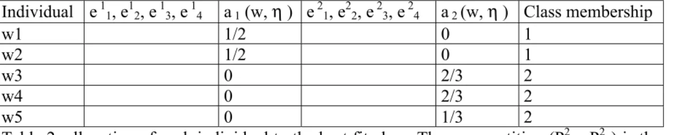
Individual e 11, e12, e 13, e 14 a 1 (w, η ) e 21, e22, e 23, e 24 a 2 (w, η ) Class membership

w1 1/2 0 1

w2 1/2 0 1

w3 0 2/3 2

w4 0 2/3 2

w5 0 1/3 2

Table 2: allocation of each individual to the best fit class. The new partition (P21 , P22) is the same

The process has converged towards the partition : (P11 , P12) = {{F1, F2 }, { F3, F4, F5}} and the

copulas W for the first class and Min for the second.

4) The special case of the standard mixture decomposition problem 4.1 Properties of a distribution base of unit mass distributions

Imbedding the standard mixture decomposition problem in the mixture decomposition of distribution of distributions problem, in the case of a unique quantitative random variable Z, is our aim in this section. Each value taken by an individual "w" can be transformed in a unique way in a distribution which takes the value 0 until Z (w) not included and the value 1 after. Such distribution is called "unit mass". More formally, if Ω = {w1,…,wn} and Z(wi) = zi, the distribution Fi

associated to wi is defined by F i (t) = Pr (X i ≤ t) where the random variable X i associated to wi is

such that its distribution Fi satisfies: Fi(t) = 0 if t < zi and Fi(t) = 1 if t ≥ zi . If the distribution base F

contains only such distributions Fi, Fz is the distribution associated to the random variable Z and the

Ti increases with i, we have the following results:

Proposition 7

1) If H(x1,…,xp) = C(G T1(x1) ,…, G Tp(xp) ) then C is the Min copulas.

2) If xp < 1, then Min (G T1(x1) ,…, G Tp(xp) ) = G Tp(xp).

3) If x< 1 then G T(x) = Prob ( Z > T)= 1-Fz (T) .

4) If xp < 1 then Fz (Tp) = 1- H(x1,…,xp).

Proof Lemma

If F is a set of unit mass distributions , x i ∈ [0, 1[ for i = 1,j, A j = {f∈ F/ f(T j) = 0} and

B j = {f∈ F/ f(T i) ≤ x i , 1≤ i ≤ j }, then we have: A j = B j and A j = Min i = 1,j Ai .

Proof

Bj ⊆ Aj as f ∈ Bj implies f ∈ F and f(Tj) < xj by definition of Bj. As F is a set of unit mass

distributions and x j ∈ [0, 1[, we have necessarily f(Tj) = 0. Therefore f ∈ A j .

Aj⊆ Bj as f ∈ Aj implies f(Tj) = 0 which implies f(Ti)= 0 for i = 1,j as f is increasing as it is a

distribution. So f ∈ Bj and therefore A j = B j . As by definition of Bj we have Bj = ∩i=1,j A i and

moreover we have proved that Aj ⊆ Bj, it results that A j = Min i = 1,j Ai .

With this lemma, we can now prove the proposition 7.

1) If H(x1,…,xp) = C(G T1(x1) ,…, G Tp(xp) ) then C is the Min copulas.

This can be proved in the following way: if all xi are equal to 1, as all the elements of a distribution

base take a value smaller than 1 everywhere, we have by definition of a point distribution of distributions: GTi(xi) = 1 and also, by definition of a k-point joint distribution of distribution

H(x1,…, xp) = 1. So, in that case 1) is true. Suppose now that some xi are smaller than 1 and

suppose by denoting them x'1,…,x'j such that their corresponding T denotedT '1,…,T'j are

distributions included in the distribution base, which are lower than x'1,…,x'j are the same as the

ones which are also lower than x1,…,xp. We can now apply the lemma 1 by denoting

A j = {f∈ F/ f(T' j) = 0} and B j = {f∈ F/ f(T' i) ≤ x' i , 1≤ i ≤ j } . As G T' j(x'j) = {f∈ F/ f(T' j) = 0} 

/ F  and H(x'1,…,x'j) = {f∈ F/ f(T' i) ≤ x' i , 1≤ i ≤ j } / F , it results that G T' j(x'j) = A j/ F ,

and H(x'1,…,x'j) = B j/ F . As from the lemma we have A j = B j it results that G T'j(x'j) =

H(x'1,…,x'j) and so, G T'j(x'j) = H(x1,…,xp). From the lemma, we have also A j = Min i = 1,j Ai 

which implies , G T' j(x'j) = Min i = 1,j G T'i(x'i) . As Mini = 1,j G T'i(x'i) = Mini = 1,p G Ti(xi) (as for the i

such that xi = 1 we have G Ti(xi) = 1 and for the i such that xi < 1 we have G Ti(xi) ≤ 1), we get

H(x1,…,xp) = Mini = 1,p G Ti(xi) which shows that H(x1,…,xp) = C(G T1(x1) ,…, G Tp(xp) ) where C is

the Min copulas.

2) If x p < 1, then Min (G T1(x1) ,…, G Tp(xp) ) = G Tp(xp).

As in the proof of 1) we denote x'1,…,x'j (associated to increasingT'1,…,T'j),the xi among x1,…,xp

which are strictly lower than 1. It results that x'j = xp and so from lemma 1 that Min (G T1(x'1) ,…,

G Tp(x'j)) = G Tp(xp). We have

Min (G T 1(x1) ,…, G Tp(xp)) = Min (G T'1(x'1) ,…, G T'j(x'j)) as shown in the preceding proof

.Therefore we get finally: Min (G T1(x1) ,…, G Tp(xp) ) = G Tp(xp).

3) If x< 1 then G T(x) = Prob ( Z > T) = 1-Fz (T) as by definition Fz (T) = Pr ({Z(w) ≤ T } ) and

G T (x) = Pr ({F i ∈ F / F i (T) ≤ x } ) is exactly the proportion of unit mass distributions Fi which

value is Fi(t) = 1 only strictly after T (i.e. t > T), as Fi(t) = 0 if t < Z(wi) and Fi(t) = 1 if t ≥ Z(wi). In

other words, this means that G T(x) is the proportion of individuals w such that Z(w) > T.

4) If xp < 1 then Fz (Tp) = 1- H(x1,…,xp) as from 1), H(x1,…,xp) = Min(G T1(x1) ,…, G Tp(xp) ) and

from 2), Min(G T1(x1) ,…, G Tp(xp) ) = G Tp(xp) and from 3) Fz (Tp)= 1- G Tp (x).

4.2 The standard mixture decomposition problem is a special case

Here we need to introduce the following notations: Fzi is the distribution associated to a quantitative

random variable Zi defined on Ω = {w1,…,wn}. Fi is a distribution base whose elements are the unit

mass distributions associated to each value Zi(wi) (i.e. they take the value 0 for t ≤ Zi(wi) and 0 for

t< Zi(wi)). GiT is a point-distribution of distributions at point T associated to the distribution base

Fi. HiT1,…,T k is a k-point joint distribution of distributions associated to the same distribution base.

Proposition 8

If H T1,…,T k = ∑i=1,p pi HiT1,…,T k with ∑i=1,p pi = 1, then Fz = ∑i=1,p pi Fzi .

Proof

From the proposition 2, we have HiT1,…,T k (x1,…,xp) = C i ( GiT1(x1) ,…, GiTp(xp)) where C i is a

p-copula. Therefore H T1,…,T k (x1,…,xp) = ∑i=1,p pi C i ( GiT1(x1) ,…, GiTp(xp)).

We choose xp < 1 and we use 1), 2), 3),4) in proposition 7.

From 1) we get: H T1,…,T k (x1,…,xp) = ∑i=1,p pi Min( GiT1(x1) ,…, GiTp(xp)) .

From 3) we get: H T1,…,T k (x1,…,xp) = ∑i=1,p pi (1-Fzi(Tp))= 1-∑i=1,p pi Fzi (Tp) .

From 4) we have Fz (Tp) = 1- H(x1,…,xp) and therefore Fz (Tp) = ∑i=1,p pi Fzi (Tp).

As the same reasoning can be done for any sequence T1,…,T p, it results finally that:

Fz = ∑i=1,p pi Fzi .

4.3 Links between the generalised mixture decomposition problem and the standard one

It results from the proposition 8 that by solving the mixture decomposition of distribution of distributions problem we solve the standard mixture decomposition problem. This results from the fact that it is possible to induce Fzi (T1),..., Fzi (Tp), from Gi T1(x1) ,…, GiTp(xp) and therefore, the

parameters of the chosen model of the density law associated to each Zi. Moreover, by choosing the "best model" among a given family of possible models (Gaussian, Gamma, Poisson,…) for each Zi, we can obtain a different model for each law of the mixture. "Best model" means the

Gaussian , Gamma or Poisson,… model which fit the best with Fzi (T1),..., Fzi (Tp) for each i. It

would be interesting to compare the result of both approach: the mixture decomposition of a distribution of distributions algorithms, and the standard mixture distribution algorithms in the standard framework, when the same model is used for each class or more generally when each law of the mixture follows a different family model.

Conclusion

Many things remain to be done. For instance, to compare the results obtained by the general methods and the standard methods of mixture decomposition on standard data. We have considered the mixture decomposition problem in the case of a unique variable. In order to extend it to the case of several variables, we can proceed as follows: we look for the variable which gives the best mixture decomposition criteria value in two classes and we repeat the process to each class thus obtained until the size of the classes becomes to small. To extend the methods to the case where each class may be modelled by a different copula family. Also, the GT can be modelled at each T

by a different distribution family. We can also add other criteria taking care of a class variable and a learning set. Notice that the same approach can be used in the case where instead of having distributions we have any kind of mapping. For example, if each unit is described by a trajectory of a stochastic random process XT, then each GT is the distribution of XT. We can then apply the same

general approach in order to obtain classes of units characterised by copulas. For instance, in case of a Markov process, each class can satisfy a copula Cst = Csu*Cut . Instead of ditributions GTn(x)

with Tn and x ∈ IR we can generalise to Tn and x ∈ IRn.

References

Bandemer and Nather (1992) "Fuzzy Data Analysis". Kluwer Academic Publisher.

Bock H.H., Diday E. (eds.) (2000) "Analysis of Symbolic Data.Exploratory methods for extracting statistical information from complex data".Springer Verlag, Heidelberg, 425

Celeux G., Govaert G. (1993) "Comparison of the Mixture and the classification maximum likelihood in cluster analysis". Journal Statist. Computer, 47, 127-146.

Celeux G., Diebolt J. (1986) L'algorithme SEM: un algorithme d'apprentissage probabiliste pour les mélanges de lois de probabilité. Revue de Statistique Appliquée. Vol 34, n°2.

Clayton D.G. (1978) "A model for association in bivariate life tables". Biometrika 65, 141-151. Darsow W., Nguyen B., Olsen E. (1992) "Copulas and Markov processes". Illinois J. Math. 36, 600-642.

Dempster A.P., Laird N.M., Rubin D.B. (1977) "Mixture densities, maximum likelihood from incomplete data via the EM algorithm" Journal of the Royal Stat. Society, 39, 1, 1-38.

Diday (1971) "Une nouvelle méthode en classification automatique et reconnaissance des formes". Revue de Statistiques Appliquée, 19, 2 Diday and al (1980) Optimisation en classification automatique. INRIA edit 78150 Rocquencourt (France) (Two Books , 896 pages).

Diday (1998) "Extracting Information from Multivalued Surveys or from Very Extensive Data Sets by Symbolic Data Analysis" Advances in Methodology, Data Analysis and Statistics. Anuska Ferligoj (Editor), Metodoloski zveski, 14. ISBN 86-80227-85-4.

Diday E., Ok Y., Schroeder A. (1974) "The dynamic clusters method in Pattern Recognition". Proceedings of IFIP Congress, Stockolm.

Diday (1998) "Extracting Information from Multivalued Surveys or from Very Extensive Data Sets by Symbolic Data Analysis" Advances in Methodology, Data Analysis and Statistics. Anuska Ferligoj (Editor), Metodoloski zveski, 14. ISBN 86-80227-85-4.

Diday E., Ok Y., Schroeder A. (1974) "The dynamic clusters method in Pattern Recognition". Proceedings of IFIP Congress, Stockolm.

A.K. Jain , R. C. Dubes (1988) "Algorithms for Clustering Data". Prentice Hall Advanced Reference Series.

Janowitz M., Schweitzer B. (1989) "Ordinal and percentile clustering". Math. Social Sciences. 18, 135-186.

Menger K. (1949) "The theory of relativity and geometry in Albert Einstein? Philosopher-Scientist, Library of Living Philosophers, ed. by P.S. Schilp, Evanston, IL, VII,459-474.

Nelsen R.B.(1998) "An introduction to Copulas" in Lecture Notes in Statistics. Springer Verlag. Tassi Ph., Legait S. (1990) "Théorie des probabilités, en vue des applications statistiques". Editions technip.