HAL Id: hal-01359237
https://hal.archives-ouvertes.fr/hal-01359237
Submitted on 2 Sep 2016
HAL is a multi-disciplinary open access archive for the deposit and dissemination of sci-entific research documents, whether they are pub-lished or not. The documents may come from teaching and research institutions in France or
L’archive ouverte pluridisciplinaire HAL, est destinée au dépôt et à la diffusion de documents scientifiques de niveau recherche, publiés ou non, émanant des établissements d’enseignement et de recherche français ou étrangers, des laboratoires
Localization of Distributed EEG Sources in the Context
of Epilepsy: A Simulation Study
Hanna Becker, Laurent Albera, Pierre Comon, Rémi Gribonval, Fabrice
Wendling, Isabelle Merlet
To cite this version:
Hanna Becker, Laurent Albera, Pierre Comon, Rémi Gribonval, Fabrice Wendling, et al.. Localization of Distributed EEG Sources in the Context of Epilepsy: A Simulation Study. Innovation and Research in BioMedical engineering, Elsevier Masson, 2016, 37 (5-6), pp.242-253. �10.1016/j.irbm.2016.04.001�. �hal-01359237�
Localization of distributed EEG sources in the context
of epilepsy: a simulation study
Hanna Beckera,∗, Laurent Alberab,c,d, Pierre Comone, R´emi Gribonvald, Fabrice Wendlingb,c, Isabelle Merletb,c
aTechnicolor R&D France, F-35576 Cesson-S´evign´e, France bINSERM, U1099, Rennes, F-35000, France cUniversit´e de Rennes 1, LTSI, Rennes, F-35000, France d Centre INRIA Rennes-Bretagne Atlantique, Rennes, F-35042, France eGipsa-Lab, CNRS, University of Grenoble Alpes, F-38000 Grenoble, France
Abstract
Objective: Surface EEG recordings are routinely performed for the diagnosis and management of epilepsy. More particularly, they can help to delineate the brain regions involved in interictal epileptic activity. This is achieved by applying distributed source localization algorithms to the EEG data. Over the last two decades, a multitude of different methods have been proposed. The objective of this paper consists in comparing the performance of eight representative algorithms taking into account recently developed methods.
Methods: The performance comparison is based on realistic computer simulations in the context of epileptic source localization.
Main findings: All tested algorithms generally permit to identify the source positions, but only some algorithms (STWV-DA, 4-ExSo-MUSIC, SVB-SCCD, cLORETA) also give an indication of the spatial extent of the sources. Localizing deep and mesial sources remains a challenging problem.
∗Corresponding author: Hanna Becker, Technicolor R&D, 975, Avenue des Champs
Keywords: EEG, distributed source localization, epilepsy, brain source imaging
1. Introduction
Surface ElectroEncephaloGraphy (EEG) recordings permit to collect valu-able information about the cerebral sources that are at the origin of the observed electromagnetic brain activity. This information is crucial for the diagnosis and management of some diseases. In this paper, we focus in partic-ular on the application of EEG in the context of epilepsy, where the objective consists in identifying the brain regions which are involved in epileptic ac-tivity between seizures. The precise delineation of these areas is essential for the evaluation of patients with drug-resistant partial epilepsy for whom a surgical intervention can be considered to remove the epileptogenic brain regions that are responsible for the occurrence of seizures. To this end, source localization techniques are applied to interictal spikes as has been done in several previous studies [1, 2, 3, 4, 5, 6]. Most of these studies have focused on identifying equivalent current dipoles, each of which summarizes the epilep-tic activity in a certain brain area. Yet it has been shown that the epilepepilep-tic paroxysms which are observable by EEG measurements often involve large cortical regions [7, 4, 8, 9, 10]. Therefore, our goal is not only to identify the locations of the epileptic regions, but also to determine their spatial extents. This is achieved by localizing distributed sources, which are characterized by a high number of dipoles (largely exceeding the number of sensors) with fixed locations.
which is recorded by the EEG sensors is also referred to as brain source imag-ing and requires solvimag-ing an ill-posed inverse problem. In order to restore iden-tifiability, additional hypotheses about the sources have to be made. Over the past two decades, a multitude of brain source imaging algorithms have been proposed (see, e.g., [11, 12, 13, 14]), that differ essentially in the exploited hy-potheses as well as in methodological aspects. In [14], these approaches have been dinstinguished into four groups: regularized least squares, Bayesian, tensor-based, and extended source scanning methods. Even though several studies [15, 16, 12, 17, 14] have aimed at comparing different source imaging algorithms, a full and deep study of these methods that takes into account recent advances in this field is still missing. The objective of this paper is to conduct a thorough, comparative simulation study with eight representa-tive algorithms belonging to different classes of source imaging approaches. This study extends the preliminary results reported in [14] by considering a significantly wider panel of scenarios and an updated list of algorithms.
2. Materials and methods
2.1. Data model
The brain electric and magnetic fields are generated by the current flows that result from the electrochemical process of information transmission be-tween neurons. To obtain a signal of sufficient amplitude to be measurable at the surface of the scalp, a certain number of simultaneously active neuronal populations is required. These populations can be modeled by a number of current dipoles belonging to a pre-defined source space. As the EEG record-ings are mostly generated by pyramidal cells located in the gray matter with
an orientation perpendicular to the cortex [18], it is physiologically plausible to assume that the D dipoles of the source space are located on the cortical surface with fixed orientations perpendicular to this surface. The electric po-tential data that is recorded at the N electrodes of an EEG sensor array for T time samples then constitutes the superposition of all source dipole signals contained in the signal matrix S ∈ RD×T that are transmitted to the surface of the scalp. The propagation of the signals in the head volume conductor is characterized by the lead field matrix G ∈ RN ×D. This leads to the following model for the EEG data:
X = GS. (1)
In the context of epilepsy, the epileptic regions can be modeled by dis-tributed sources that can be described as the union of (one or) several con-tiguous areas of the cortex (so-called patches) with highly correlated source activities [19, 6]. All dipoles that do not belong to a distributed source can be considered to emit a background activity. Consequently, to distinguish between the P distributed sources, that we want to retrieve, and the noisy background activity, we can rewrite the data model (1) in the following way:
X = P X p=1 X kp∈Ωp gkps T kp + X l /∈∪P p=1Ωp glsTl = Xe+ Xb. (2)
Here, Ωp is the set of indices of the dipoles that belong to the p-th distributed source, gk is the lead field vector of the k-th dipole, and sk is the associated signal vector that corresponds to the k-th row vector of S. The matrices Xe and Xb contain the epileptic and background activity, respectively.
For a given head model and source space, the lead field matrix G can be computed numerically [20]. Therefore, we assume in this paper that it
is known. The objective of brain source imaging then consists in estimating the unknown sources S from the measurements X. As the number of source dipoles D (several thousands) is much higher than the number of sensors (several hundreds), the lead field matrix is severely underdetermined, making the inverse problem ill-posed. In order to restore identifiability, additional hypotheses about the sources have to be made, giving rise to a large number of different source imaging algorithms.
2.2. Algorithms
In this paper, we concentrate on the following eight source imaging al-gorithms: sLORETA, cLORETA, MCE, SVB-SCCD, MxNE, Champagne, 4-ExSo-MUSIC, and STWV-DA.
The first five methods belong to the class of regularized least squares approaches. More particularly, sLORETA [21] employs an L2-norm regu-larization strategy like the classical minimum norm estimate and normalizes the solution with respect to the estimated noise level. cLORETA [22] aims at identifying a spatially smooth source distribution by applying a Lapla-cian operator L to the source matrix in the L2-norm regularization term. MCE [23] identifies a sparse source estimate by replacing the L2-norm in the regularization term by an L1-norm. SVB-SCCD [24] leads to a piece-wise constant source estimate, which is obtained by employing L1-norm regular-ization both in the original source domain and on the variational map, which characterizes the changes in amplitude between adjacent source dipoles. Fi-nally, the MxNE algorithm [25] assumes that the active source dipoles do not change over the considered time interval, which is imposed using a mixed norm (L12-norm) regularization strategy.
The Champagne algorithm [26] is a representative of empirical Bayesian methods, which are based on a probabilistic model of the data. Assuming that the sources at each time point are described by a zero-mean Gaussian random vector with independent elements, the goal of the algorithm is to obtain an estimate for the source covariance matrix, which can then be used to infer an estimate of the sources.
4-ExSo-MUSIC [6] is an extended source scanning method, which is based on the quadricovariance matrix containing the fourth order cumulants esti-mated from the data. More particularly, it extends the classical MUSIC algorithm, which has previously been used for equivalent dipole localization, to the identification of distributed sources based on higher order statistics by employing a dictionary of circular-shaped source regions of varying positions and sizes, the so-called disks.
STWV-DA [27] is a tensor-based source imaging algorithm, which pro-ceeds in two steps. The first step consists in separating several simultaneously active distributed sources based on tensor decomposition of space-time-wave-vector data. In the second step, the results of the tensor decomposition are used for source localization, which is performed for each distributed source separately based on a dictionary of disks similar to 4-ExSo-MUSIC.
2.3. Simulation setup 2.3.1. Data generation
We simulate physiologically plausible EEG recordings for an electrode cap comprising N = 91 electrodes and data intervals with a length of T = 200 time samples at a sampling frequency of 256 Hz. To this end, we consider a realistic head model composed of three compartments representing the
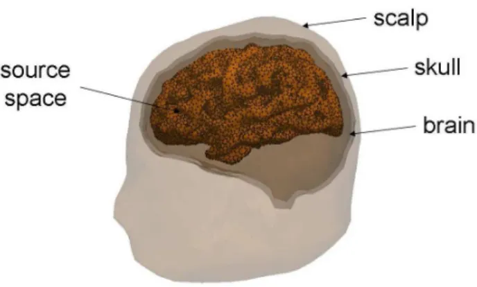
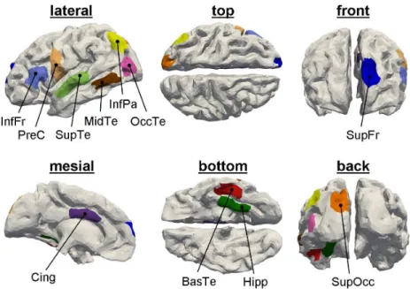
brain, the skull, and the scalp (see Fig. 1), which have been derived from a single subject MRI. The source space is defined by the triangularized inner cortical surface (gray matter / white matter interface), segmented from the same MRI. A grid dipole is placed at the centroid of each of the triangles with an orientation perpendicular to the triangle’s surface. The grid consists of 19626 triangles and on average, each triangle describes 5 mm2 of the cortical surface. The lead field matrix G is then computed numerically using a boundary element method (ASA, ENT, Enschede, The Netherlands). For the generation of distributed sources, we consider 11 different patches located on the left hemisphere (see Fig. 2). Each patch consists of 100 adjacent grid dipoles corresponding to a cortical area of approximately 5 cm2.
To generate physiologically plausible brain signals, a model based on cou-pled neuronal populations [19, 7] is employed. This model is used to simulate interictal epileptiform spike-like signals for the source dipoles belonging to the patches and normal background activity of the brain for all other dipoles.
2.3.2. Tested methods
All source imaging algorithms are applied to spatially prewhitened data, except for Champagne, which directly uses the noise covariance instead. The noise covariance matrix is estimated using 25000 time samples of data gen-erated for the case where all dipoles emit background activity. To improve the SNR, we average the data of 10 spikes. Since sLORETA, cLORETA, MCE, and SVB-SCCD do not take into account the temporal information, they are applied to the time sample corresponding to the maximum of the epileptiform spike. STWV-DA, MxNE and Champagne are applied to the 200 time samples of averaged epileptic activity. For 4-ExSo-MUSIC, to have
a sufficient amount of time samples at our disposal to accurately estimate the fourth order statistics, we concatenate the 200 time samples that are selected for each of the 10 spikes, leading to a total of 2000 time samples.
The algorithms are implemented as follows: for sLORETA and cLORETA, the regularization parameter is fixed such that it approximately balances be-tween the data fit and the regularization term. MCE and MxNE are imple-mented using FISTA [28]. The regularization parameter is chosen according to the level of sparsity that we aim to achieve. SVB-SCCD is implemented as described in [24]. The implementation of Champagne follows [26], but has been modified to take into account the fixed orientations of the source dipoles. For STWV-DA, the tensor is constructed and decomposed as described in [27] with a number of components that is equal to the number of patches. For 4-ExSo-MUSIC, the dimension of the signal subspace is chosen accord-ing to the number of patches. For both STWV-DA and 4-ExSo-MUSIC, we construct a dictionary of disks comprising up to 100 grid dipoles.
2.3.3. Evaluation criteria
To quantitatively evaluate the performance of the algorithms, we use two measures1: the Distance of Localization Error (DLE) [29], which character-izes the difference between the original and the estimated source configura-tions, and the Receiver Operating Characteristic (ROC) [16], which reflects the ability of a source imaging algorithm to recover the extent and the form of the distributed sources.
1In the online supplementary material, a third evaluation criterion, the Patch Center
Distance (PCD), which is independent of the patch size, is considered, but as the findings are similar to those of the DLE and ROC, they are not reported in the main article.
Mathematically, the DLE is defined as follows: DLE = 1 2 1 Q X k∈I min `∈ ˆI ||rk− r`||2 + 1 ˆ Q X `∈ ˆI min k∈I ||rk− r`||2 (3)
where I denotes the set of indices of all grid dipoles belonging to an active patch, Q is the number of active grid dipoles, i.e., Q = #I, ˆI denotes the set of indices of all estimated active source dipoles and ˆQ = # ˆI corresponds to the number of the latter. Furthermore, rk denotes the position of the k-th source dipole. To compare the estimated source configuration to the original source configuration characterized by the dipoles belonging to the active patches, we consider a number of active estimated dipoles that is equal to the true number of patch dipoles or as close to this number as possible. To achieve this, we threshold the absolute value of the sLORETA, cLORETA, and SVB-SCCD solutions and the STWV-DA, and 4-ExSo-MUSIC metrics by a suitable value. In case of MCE and MxNE, we choose the regularization parameter to obtain a number of non-zero elements that lies between 80 % and 100 % of the number of active sources.
The ROC displays the True Positive Fraction (TPF) of correctly identi-fied source dipoles as a function of the False Positive Fraction (FPF), which represents the number of source dipoles erroneously associated with the dis-tributed sources:
TPF = #(I ∩ ˆI)
#I ; FPF =
# ˆI − #(I ∩ ˆI)
#J − #I . (4) Here, J denotes the set of all dipoles belonging to the source space. Different TPF and FPF values are achieved by varying the threshold values for the extended source localization algorithms. The results are averaged over 50 realizations with different spike-like signals and varying background activity.
3. Results
3.1. Influence of the patch position
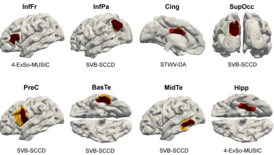
Superficial sources exhibit more focal distributions of the electric poten-tial than deep sources. Furthermore, the signals emanating from deep sources lead to smaller amplitudes at the sensor level (and thereby, smaller SNRs) than those of superficial sources. It is thus significant to determine the influ-ence of the patch position on the localization accuracy of the different source imaging methods. To this end, we consider 8 different patches: InfFr, InfPa, Cing, SupOcc, PreC, BasTe, MidTe, and Hipp. The results in terms of ROC curves and DLE are shown in Fig. 3 and Table 1, respectively. The patches that are recovered by the algorithm which yields the highest TPF at an FPF of 0.2 % are shown in Fig. 4 in comparison to the original patches.
For patches InfPa, SupOcc, BasTe, and MidTe, the best results in terms of both DLE and ROC are achieved by SVB-SCCD, whereas STWV-DA and 4-ExSo-MUSIC yield the best performance for patches InfFr, Cing, PreC, and Hipp. These two methods lead to almost identical source imaging re-sults because in the case of single patches, there is no source separation to be performed by STWV-DA and the patch estimates are mostly influenced by the employed dictionary of disks, which is the same for STWV-DA and 4-ExSo-MUSIC. sLORETA and cLORETA generally yield better results in terms of both DLE and ROC than MCE and MxNE. Surprisingly, MCE slightly outperforms MxNE for all tested scenarios, whereas one could have expected that the exploitation of temporal information would lead to more robust source estimates. However, this result could be related to our some-what abusive use of the sparse source estimation techniques to recover patches
of larger extent. Champagne leads to intermediate DLEs because it always identifies a small number of dipoles at the correct source position. Albeit, as the ROC curves show, this method is the least suited to recover the spatial extent of the patches because it recovers very sparse source estimates.
Concerning the patch location, the examined source imaging algorithms generally yield good results for superficial patches (InfFr, InfPa, SupOcc, and MidTe) with exception of patch PreC. However, the algorithms exhibit some difficulties for accurately recovering deep patches such as BasTe and Hipp, as well as for the patch Cing, located between the two hemispheres.
3.2. Influence of the patch size
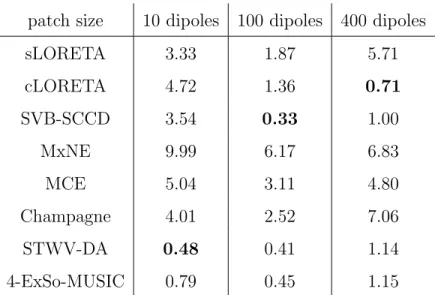
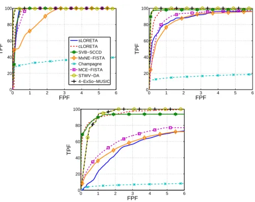
To determine the influence of the source extent on the performance of the different source imaging algorithms, we vary the size of the patch SupFr and consider three patches composed of 10, 100, and 400 grid dipoles corre-sponding to an area of approximately 50, 500 and 2000 mm2. The simulation results in terms of ROC curves, estimated source reconstructions, and DLE values are shown in Fig.s 5 and 6, and Table 2, respectively.
The performance of sLORETA, Champagne, MCE, and MxNE in terms of ROC decreases as the patch area increases. This is due to the fact that these methods, especially MCE and MxNE, are conceived for focal sources and are not well suited to recover the spatial extent of the sources. 4-ExSo-MUSIC, STWV-DA, and SVB-SCCD on the other hand have been developed to localize distributed sources and can therefore accurately recover sources of larger size. The hypothesis of spatial smoothness exploited by cLORETA also favors the reconstruction of extended sources, leading to the best performance among all tested methods for the largest considered patch.
In terms of DLE, all methods except for cLORETA yield the highest reconstruction accuracy for a patch of medium size. For cLORETA, we observe a continually decreasing DLE for augmenting patch size. For the smallest patch, the best source reconstructions are achieved by STWV-DA and 4-ExSo-MUSIC. The source dipoles of maximal amplitudes identified by Champagne, MCE, and MxNE are close to the true patch, but not exactly at the correct position. Furthermore, SVB-SCCD overestimates the size of the patch, recovering a much larger source region, as is the case for sLORETA and cLORETA. In fact, these three methods yield nearly the same estimated source distributions for the patches of small and medium sizes. These source reconstructions are better suited for the medium-sized patch, which leads to smaller DLE in this case. In particular, SVB-SCCD achieves the best DLE of all methods for the medium-sized patch. Note that sLORETA, cLORETA, MCE, and MxNE also identify several dipoles on the right hemisphere, un-like the distributed source localization algorithms SVB-SCCD, STWV-DA, and 4-ExSo-MUSIC. Nevertheless, for cLORETA, the amplitudes of the con-tralateral source dipoles are rather small. For the largest patch, cLORETA and SVB-SCCD outperform all other tested methods. While the sLORETA solution indicates also a patch of larger extent, the sparse estimates obtained by MCE, MxNE, and, in particular, Champagne are not suited to determine the shape of the patch and would rather suggest the existence of several distinct point sources.
3.3. Influence of the patch number
In practice, one is often confronted with measurements that originate from several quasi-simultaneous active source regions within the brain. In this
section, we analyze the ability of the source imaging algorithms to identify two or three patches that are involved in epileptic spike propagation.
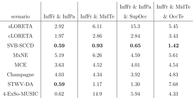
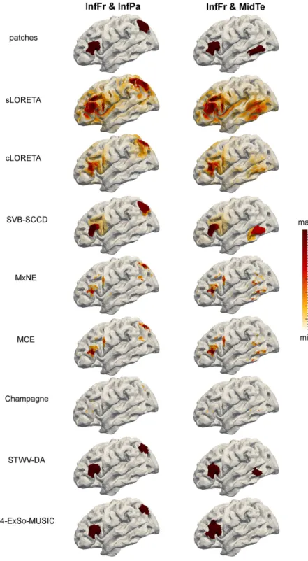
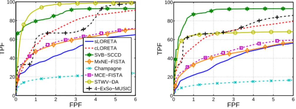
First, we consider two scenarios with two patches of medium distance: scenario InfFr & InfPa and scenario InfFr & MidTe. We use the same signals for the dipoles of both patches except for a 3 to 4 sample delay from one patch to another. The source imaging performances in terms of ROC, reconstructed sources, and DLE are shown in Fig. 7 and 8, and Table 3, respectively. The patch MidTe is partly located in a sulcus (cf. Fig. 2), leading to weaker surface signals than the patches InfFr and InfPa, which are mostly on a gyral convexity. This results in a deterioration of the performance of all source imaging algorithms, except for SVB-SCCD and Champagne, for the scenario InfFr & MidTe compared to the scenario InfFr & InfPa. More particularly, for the scenario InfFr & InfPa, all source imaging algorithms exhibit high dipole amplitudes for dipoles belonging to each of the true patches, whereas for the scenario InfFr & MidTe, the weak patch is less visible on the estimated source distributions of cLORETA, MCE, and MxNE, slightly better visible on the sLORETA solution, but completely missing for 4-ExSo-MUSIC. SVB-SCCD and STWV-DA both recover the patch MidTe, but with smaller amplitude in case of SVB-SCCD and smaller size for STWV-DA.
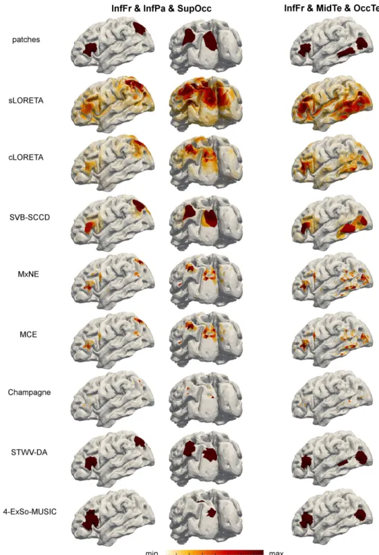
Next, we study two three-patch scenarios: InfFr & InfPa & SupOcc and InfFr & MidTe & OccTe. We consider a delay of 3 to 4 samples between the signals of the first two patches and a delay of 5 to 6 samples between the signals of the first and third patch. For the resulting ROC curves, source reconstructions, and DLEs, see Fig. 9 and 10, and Table 3. The best re-sults are achieved by SVB-SCCD, followed by STWV-DA and cLORETA.
STWV-DA leads to good results for the scenario InfFr & InfPa & SupOcc, but underestimates the extent of the patch MidTe for the scenario InfFr & MidTe & OccTe. For this scenario, STWV-DA also identifies several spurious source regions of small size located between the patches MidTe and InfFr. for some realizations. The cLORETA solution exhibits dipoles with high am-plitudes at all three patch positions, but makes it difficult to determine the patch shape. The same problem is exacerbated for MxNE, MCE, and Cham-pagne, which additionally identify a number of scattered dipoles around the three foci of brain activity. This explains the reduced performance compared to SVB-SCCD. 4-ExSo-MUSIC yields similar results to STWV-DA for the scenario InfFr & InfPa & SupOcc, but overestimates the size of the patch InfFr while recovering a smaller area for the patch SupOcc. In addition, the estimated source region corresponding to patch InfPa is not at the correct position, leading to a higher DLE and worse ROC curve than STWV-DA. For scenario InfFr & MidTe & OccTe, 4-ExSo-MUSIC recovers only one of the two patches located in the temporal lobe, namely the patch OccTe. Fi-nally, sLORETA leads to blurred source reconstructions and does not permit to discern the close patches InfPa and SupOcc or MidTe and OccTe.
4. Discussion
In summary, for the considered scenarios, sLORETA, Champagne, MCE, and MxNE recover well the source positions, though not their spatial extents as they are conceived for focal sources, while 4-ExSo-MUSIC, STWV-DA, and SVB-SCCD also permit to obtain an accurate estimate of the source size. cLORETA leads to intermediate results as the identified dipoles with high
amplitudes and smooth source distributions correspond well to the patches, but make it difficult to delineate the source regions. Nevertheless, the spatial smoothness prior has proven to be especially effective for large patch sizes where cLORETA achieves the best performance in terms of DLE.
Among the methods for focal source reconstruction, Champagne leads to the sparsest source distributions, identifying only a very small number of dipoles. This result might be explained by the fact that Champagne is based on the assumption that all grid dipoles emit independent source activities, which is violated by the patches. Moreover, in the Champagne algorithm, there is no parameter that can be adjusted to obtain different levels of spar-sity, contrary to MCE and MxNE where this is achieved by varying the regu-larization parameter. At the same time, this is also an important advantage of Champagne because in practice, the tuning of parameters is tedious and time-consuming, and even though Champagne does not identify the source extents, it still permits to accurately localize the foci of the source activ-ity. Combined with an adequate scheme for distributed source localization, Champagne could thus become a powerful tool for source imaging.
While STWV-DA and 4-ExSo-MUSIC lead to similar patch estimates for the single patch scenarios and in some cases also for multipatch scenarios, all in all, STWV-DA outperforms 4-ExSo-MUSIC as it leads to better source estimates in the presence of multiple patches, where 4-ExSo-MUSIC does not localize all patches or leads to erroneous patch estimates. This problem is due to the limitation of the employed dictionary to distributed sources composed of one disk and could be overcome by modifying the dictionary to include combinations of several disks. However, this has not been done so
far. Compared to SVB-SCCD, STWV-DA only leads to better results for the smallest considered patch. Otherwise, SVB-SCCD yields slightly better source estimates than STWV-DA, which is due to its greater flexibility in recovering the patch shape. Because of the use of a dictionary of disks, STWV-DA tends to recover circular-shaped source regions.
Even though this has not been explicitly shown in the above simula-tions, we noticed that most of the methods except for STWV-DA require prewhitening of the data or a good estimate of the noise covariance matrix (in case of Champagne) in order to yield accurate results. On the one hand, this can be explained by the assumption of spatially white Gaussian noise made by some approaches, while on the other hand, the prewhitening also leads to a decorrelation of the rows of the lead field matrix and therefore to a better conditioning of the lead field matrix, which consequently facilitates the correct identification of active grid dipoles.
5. Conclusion
We have compared eight source imaging algorithms using realistic sim-ulated EEG data in the context of epilepsy. We have observed that these methods generally work well for superficial patches, but have difficulties in identifying deep patches and mesial sources, located close to the midline. While all algorithms generally permit to identify the source positions, only STWV-DA, 4-ExSo-MUSIC, SVB-SCCD, and, to some extent, cLORETA, also give an indication of the spatial extent of the sources. On the whole, for the situations addressed in our simulation study, STWV-DA and SVB-SCCD seem to be the most promising algorithms for distributed source localization.
Acknowledgements
H. Becker was supported by Conseil R´egional PACA and by CNRS France. The work of P. Comon was funded by the FP7 European Research Council Programme, DECODA project, under grant ERC-AdG-2013-320594. The work of R. Gribonval was funded by the FP7 European Research Council Programme, PLEASE project, under grant ERC-StG-2011-277906. Further-more, we acknowledge the support of Programme ANR 2010 BLAN 0309 01 (project MULTIMODEL).
Conflicts of interest
None.
References
[1] J. S. Ebersole, Noninvasive localization of epileptogenic foci by EEG source modeling, Epilepsia 41 (2000) S24 – 33.
[2] I. Merlet, Dipole modeling of interictal and ictal EEG and MEG, Epilep-tic Disord Special Issue (2001) 11 – 36.
[3] C. M. Michel, M. M. Murray, G. Lantz, S. Gonzalez, L. Spinelli, R. G. D. Peralta, EEG source imaging, Clinical Neurophysiology 115 (10) (2004) 2195–2222.
[4] M. Gavaret, J.-M. Badier, P. Marquis, A. McGonigal, F. Bartolomei, J. Regis, P. Chauvel, Electric source imaging in frontal lobe epilepsy, Journal of Clinical Neurophysiology 23 (4) (2006) 358–370.
[5] C. Plummer, A. S. Harvey, M. Cook, EEG source localization in focal epilepsy: Where are we now?, Epilepsia 49 (2) (2008) 201 – 218.
[6] G. Birot, L. Albera, F. Wendling, I. Merlet, Localisation of extended brain sources from EEG/MEG: the ExSo-MUSIC approach, NeuroImage 56 (2011) 102 – 113.
[7] D. Cosandier-Rim´el´e, I. Merlet, J. Badier, P. Chauvel, F. Wendling, The neuronal sources of EEG: Modeling of simultaneous scalp and intracere-bral recordings in epilepsy, NeuroImage 42 (1) (2008) 135–146.
[8] J. Tao, S. Hawes-Ebersole, J. Ebersole, Intracranial EEG substrates of scalp EEG interictal spikes, Epilepsia 46 (5) (2005) 669–676.
[9] I. Merlet, J. Gotman, Reliability of dipole models of epileptic spikes, Clinical Neurophysiology 110 (6) (1999) 1013 – 1028.
[10] J. S. Ebersole, Magnetoencephalography/magnetic source imaging in the assessment of patients with epilepsy, Epilepsia 38 (1997) S1– 5.
[11] S. Baillet, J. C. Mosher, R. M. Leahy, Electromagnetic brain mapping, IEEE Signal Processing Magazine 18 (6) (2001) 14–30.
[12] R. Grech, T. Cassar, J. Muscat, K. P. Camilleri, S. G. Fabri, M. Zervakis, P. Xanthopoulos, V. Sakkalis, B. Vanrumste, Review on solving the inverse problem in EEG source analysis, Journal of NeuroEngineering and Rehabilitation 5.
[13] D. Wipf, S. Nagarajan, A unified Bayesian framework for MEG/EEG source imaging, NeuroImage 44 (2009) 947 – 966.
[14] H. Becker, L. Albera, P. Comon, R. Gribonval, F. Wendling, I. Mer-let, Brain source imaging: from sparse to tensor models, IEEE Signal Processing Magazine 32 (6) (2015) 100–112.
[15] R. D. Pascual-Marqui, Review of methods for solving the EEG inverse problem, International Journal of Bioelectromagnetism 1 (1) (1999) 75 – 86.
[16] C. Grova, J. Daunizeau, J. M. Lina, C. G. B´enar, H. Benali, J. Gotman, Evaluation of EEG localization methods using realistic simulations of interictal spikes, NeuroImage 29 (3) (2006) 734 – 753.
[17] R. A. Chowdhury, J. M. Lina, E. Kobayashi, C. Grova, MEG source localization of spatially extended generators for epileptic activity: com-paring entropic and hierarchical Bayesian approaches, PLOS ONE 8 (2) (2013) 1–9.
[18] A. M. Dale, M. I. Sereno, Improved localization of cortical activity by combining EEG and MEG with MRI cortical surface reconstruction: a linear approach, Journal of Cognitive Neuroscience 5 (2) (1993) 162–176.
[19] D. Cosandier-Rim´el´e, J.-M. Badier, P. Chauvel, F. Wendling, A physio-logically plausible spatio-temporal model for EEG signals recorded with intracerebral electrodes in human partial epilepsy, IEEE Transactions on Biomedical Engineering 54 (3) (2007) 380–388.
[20] A. Gramfort, Mapping, timing and tracking cortical activations with MEG and EEG: Methods and application to human vision, Ph.D. thesis, Telecom ParisTech (2009).
[21] R. D. Pascual-Marqui, Standardized low resolution brain electromag-netic tomography (sLORETA): technical details, Methods and Findings in Experimental and Clinical Pharmacology.
[22] M. Wagner, M. Fuchs, H. A. Wischmann, R. Drenckhahn, Smooth re-construction of cortical sources from EEG and MEG recordings, Neu-roImage 3 (3) (1996) S168.
[23] K. Uutela, M. H¨am¨al¨ainen, E. Somersalo, Visualization of magnetoen-cephalographic data using minimum current estimates, NeuroImage 10 (1999) 173 – 180.
[24] H. Becker, L. Albera, P. Comon, R. Gribonval, I. Merlet, Fast, variation-based methods for the analysis of extended brain sources, in: Proc. of EUSIPCO, Lisbon, Portugal, 2014.
[25] E. Ou, M. H¨am¨al¨ainen, P. Golland, A distributed spatio-temporal EEG/MEG inverse solver, NeuroImage 44.
[26] D. Wipf, J. Owen, H. Attias, K. Sekihara, S. Nagarajan, Robust Bayesian estimation of the location, orientation, and time course of mul-tiple correlated neural sources using MEG, NeuroImage 49 (2010) 641 – 655.
[27] H. Becker, L. Albera, P. Comon, M. Haardt, G. Birot, F. Wendling, M. Gavaret, C. G. B´enar, I. Merlet, EEG extended source localization: tensor-based vs. conventional methods, NeuroImage 96 (2014) 143–157.
for linear inverse problems, SIAM Journal of Imaging Sciences 2 (1) (2009) 183–202.
[29] J. Yao, J. P. A. Dewald, Evaluation of different cortical source localiza-tion methods using simulated and experimental EEG data, NeuroImage 25 (2) (2005) 369–382.
Figure captions and tables
Figure 1
Illustration of a realistic head model with three compartments represent-ing the brain, the skull, and the scalp and a source space that consists of a large number of dipoles (represented by black dots) located on the gray matter/white matter interface.
Figure 2
Location of the 11 patches that are considered for the simulations in this paper. We provide 6 different views of the cortical surface such that all patches can be seen. For convenience, we refer to these patches using the following names that indicate the patch positions: SupFr – superior frontal gyrus, InfFr – inferior frontal gyrus, PreC – precentral gyrus, SupTe – supe-rior temporal gyrus, MidTe – middle temporal gyrus, BasTe – basal aspect of the temporal lobe, OccTe – occipital temporal junction, InfPa – inferior parietal lobule, SupOcc – superior occipital gyrus, Cing – cingulate gyrus, Hipp – para-hippocampal gyrus.
Figure 3
Illustration of the ROC curves for the different single patch scenarios.
Figure 4
Illustration of the recovered patches for the different single patch scenar-ios. Triangles belonging to the original patches are marked in red, correctly identified triangles are dark red and erroneously identified triangles are yel-low.
Figure 5
ROC curves obtained for the different source imaging methods for differ-ent sizes of the patch SupFr: (top left) 10 dipoles, (top right) 200 dipoles, (bottom) 400 dipoles.
Figure 6
Illustration of the recovered source distributions for the different patch sizes.
Figure 7
ROC curves obtained for the different source imaging methods for the scenario InfFr & InfPa (left) and the scenario InfFr & MidTe (right).
Figure 8
Illustration of the original patches and the recovered source distributions for the two considered two-patch scenarios.
Figure 9
ROC curves obtained for the different source imaging methods for the scenario InfFr & InfPa & SupOcc (left) and the scenario InfFr & MidTe & OccTe (right).
Figure 10
Illustration of the original patches and the recovered source distributions for the two considered three-patch scenarios.
patch InfFr InfPa Cing SupOcc PreC BasTe MidTe Hipp sLORETA 3.61 2.41 3.28 2.05 4.07 2.26 6.28 3.11 cLORETA 1.43 2.72 24.8 1.28 3.17 3.56 7.43 11.1 SVB-SCCD 1.06 0.13 6.44 0.37 3.33 1.41 0.74 6.22 MxNE 8.18 6.18 27.9 4.53 10.6 9.89 8.53 18.4 MCE 3.99 3.19 22.5 3.07 4.86 6.45 5.20 14.7 Champagne 4.60 4.03 2.95 2.47 2.95 2.29 4.37 4.09 STWV-DA 0.44 0.95 1.70 0.57 1.84 2.29 1.85 1.86 4-ExSo-MUSIC 0.44 0.96 1.70 0.58 1.84 2.39 1.83 1.83
Table 1: Performance of source imaging algorithms in terms of DLE (in mm) for the 8 different single patch scenarios. The DLE values are averaged over 50 realizations with different spike-like signals and varying background activity. The smallest obtained DLE value for each patch is marked in bold.
patch size 10 dipoles 100 dipoles 400 dipoles sLORETA 3.33 1.87 5.71 cLORETA 4.72 1.36 0.71 SVB-SCCD 3.54 0.33 1.00 MxNE 9.99 6.17 6.83 MCE 5.04 3.11 4.80 Champagne 4.01 2.52 7.06 STWV-DA 0.48 0.41 1.14 4-ExSo-MUSIC 0.79 0.45 1.15
Table 2: Performance of source imaging algorithms in terms of DLE (in mm) depending on the size of the patch SupFr. The DLE values are averaged over 50 realizations with different spike-like signals and varying background activity. The smallest obtained DLE value for each patch is marked in bold.
InfFr & InfPa InfFr & MidTe scenario InfFr & InfPa InfFr & MidTe & SupOcc & OccTe
sLORETA 2.92 6.11 15.3 5.45 cLORETA 1.97 2.86 2.84 3.43 SVB-SCCD 0.59 0.93 0.65 1.42 MxNE 5.19 6.26 4.59 5.61 MCE 3.63 4.52 4.01 4.54 Champagne 4.03 4.34 3.92 4.83 STWV-DA 0.59 1.17 1.30 7.68 4-ExSo-MUSIC 0.62 14.9 5.94 4.33
Table 3: Performance of source imaging algorithms in terms of DLE (in mm) for the considered scenarios with two and three patches. The DLE values are averaged over 50 realizations with different spike-like signals and varying background activity. The smallest obtained DLE value for each scenario is marked in bold.
Figure 1: Illustration of a realistic head model with three compartments representing the brain, the skull, and the scalp and a source space that consists of a large number of dipoles (represented by black dots) located on the gray matter/white matter interface.
Figure 2: Location of the 11 patches that are considered for the simulations in this paper. We provide 6 different views of the cortical surface such that all patches can be seen. For convenience, we refer to these patches using the following names that indicate the patch positions: SupFr – superior frontal gyrus, InfFr – inferior frontal gyrus, PreC – precentral gyrus, SupTe – superior temporal gyrus, MidTe – middle temporal gyrus, BasTe – basal aspect of the temporal lobe, OccTe – occipital temporal junction, InfPa – inferior parietal lobule, SupOcc – superior occipital gyrus, Cing – cingulate gyrus, Hipp – para-hippocampal gyrus.
Figure 4: Illustration of the recovered patches for the different single patch scenarios. Triangles belonging to the original patches are marked in red, correctly identified triangles are dark red and erroneously identified triangles are yellow.
0 1 2 3 4 5 6 0 20 40 60 80 100 FPF TPF sLORETA cLORETA SVB−SCCD MxNE−FISTA Champagne MCE−FISTA STWV−DA 4−ExSo−MUSIC 0 1 2 3 4 5 6 0 20 40 60 80 100 FPF TPF 0 1 2 3 4 5 6 0 20 40 60 80 100 FPF TPF
Figure 5: ROC curves obtained for the different source imaging methods for different sizes of the patch SupFr: (top left) 10 dipoles, (top right) 200 dipoles, (bottom) 400 dipoles
0 1 2 3 4 5 6 0 20 40 60 80 100 FPF TPF sLORETA cLORETA SVB−SCCD MxNE−FISTA Champagne MCE−FISTA STWV−DA 4−ExSo−MUSIC 0 1 2 3 4 5 6 0 20 40 60 80 100 FPF TPF
Figure 7: ROC curves obtained for the different source imaging methods for the scenario InfFr & InfPa (left) and the scenario InfFr & MidTe (right).
0 1 2 3 4 5 6 0 20 40 60 80 100 FPF TPF sLORETA cLORETA SVB−SCCD MxNE−FISTA Champagne MCE−FISTA STWV−DA 4−ExSo−MUSIC 0 1 2 3 4 5 6 0 20 40 60 80 100 FPF TPF
Figure 9: ROC curves obtained for the different source imaging methods for the scenario InfFr & InfPa & SupOcc (left) and the scenario InfFr & MidTe & OccTe (right).