Comparing User Behavior When Targeted Based on
Firm Inferred Interest vs. User Stated Interest
by
Yiqun Cao
B.S. in Business Administration, Carnegie Mellon University (2016)
Submitted to the Department of Management
in partial fulfillment of the requirements for the degree of
Master of Science in Management Research
at the
MASSACHUSETTS INSTITUTE OF TECHNOLOGY
February 2021
© Massachusetts Institute of Technology 2021. All rights reserved.
Author . . . .
Department of Management
December 17, 2020
Certified by. . . .
Sinan Aral
David Austin Professor of Management
Professor of IT & Marketing
Thesis Supervisor
Accepted by . . . .
Catherine Tucker
Sloan Distinguished Professor of Management
Professor of Marketing
Chair, MIT Sloan PhD Program
Comparing User Behavior When Targeted Based on Firm Inferred
Interest vs. User Stated Interest
by
Yiqun Cao
Submitted to the Department of Management on December 17, 2020, in partial fulfillment of the
requirements for the degree of
Master of Science in Management Research
Abstract
There has been a lot of discussions on giving user more control over their private informa-tion. Our paper wants to show how practices that give user more control over privacy, could facilitate collection of self-stated interest from voluntary users. This might potentially help firms to better understand users’ true interests. The paper investigates the short run and long run impact of adopting the user stated interest into ad targeting, compared with tar-geting using firm inferred user interest. It also explores the side effects on user’s overall app engagement and the possible mechanisms that associate users’ action of stating interest with impact on their interest in ads and organic contents. Results show that on average users get more interested in ads immediately after the ad targeting adopts user stated interest categories. In the long run, however, not only does the effect diminish quickly, but there is also a lasting and significantly negative effect on users’ overall app engagement, possibly because both organic content and ad targeting use the same user profile.
Thesis Supervisor: Sinan Aral
Title: David Austin Professor of Management Professor of IT & Marketing
Contents
1 Research Overview 7
1.1 Introduction . . . 7
1.2 Literature Review . . . 10
2 Data and Background 13 2.1 Current Practice on User Privacy and Ad Recommendation . . . 13
2.2 Data Description and Sampling Scheme . . . 14
2.3 Data Summary . . . 17
3 Results and Analysis 19 3.1 Model Identification . . . 19
3.2 Results . . . 22
3.3 Robustness Checks . . . 26
3.4 Heterogeneous Effects . . . 28
4 Discussions and Conclusion 33 4.1 Causal Discussion . . . 33
4.1.1 Direct Treatment Period . . . 33
4.1.2 Possible Mechanisms . . . 34
4.2 Managerial Implications . . . 35
4.3 Conclusion . . . 36
Chapter 1
Research Overview
1.1
Introduction
Identifying consumer needs and interests has been an ever-lasting marketing question. There is a famous quote from Steve Jobs: "People don’t know what they want until you show it to them" suggesting consumers’ stated wants may not accurately represent what they truly want. Amazon slogan "If you don’t listen to your customers you will fail. But if you only listen to your customers you will also fail" also hints that firms may not completely follow users’ stated needs and wants. The question of whether and how much to listen to customers has become a wonder to many firms. Luckily, some features that grant users more control over privacy provided us with an opportunity to learn users’ true interests.
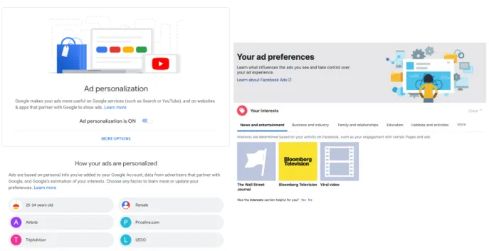
User privacy and control has become an increasingly important topic especially in this technology era, with ubiquitous use of mobile social apps that enables the easy collection of abundant individual data by technology firms. To address the user privacy concern, many firms have started adopting practices that could give user more control over their privacy. For example, in Fig. 1-1, Google has launched the Ad Personalization feature that allows users to see what their inferred tags that include both their demographics and interests. Users can delete any of these tags based on their own preference. Similarly, Facebook has launched another feature as shown on the right side of Fig. 1-1 that allows users to see their inferred interest and hence make modifications. The focus firm of our research is one of such firms that has launched a similar feature that again allows users to see what their inferred
Figure 1-1: Example of features that give users more control over their privacy interests are and hence to make changes based on their own preferences.
In this paper, we explore how to better learn users’ true interest by estimating the differ-ence between users’ ad and app engagement behavior when the firm target users based on firm’s inferred interest categories, versus based on users’ stated interest categories. Specif-ically, our focus firm (referred to as Company A in the paper) has launched an interest categories feature in a recent year that allows users to see all possible interest categories and what their inferred interest categories are based on their past behavior when using the app. Users can freely turn on or off any interest categories based on their own preferences. Once users have made changes to their interest category profile, we regard the interest categories that are opted in as user stated interest categories. We want to assess whether there is any change in users’ app engagement behavior, such as how long users view the ads and how long users use the app, after users change the inferred interest categories to their stated interest categories.
Given the endogenous nature of observational data, we employ difference-in-difference and propensity score weighting as our identification strategy. We use a reduced-form model to estimate the average treatment effect on the treated. We mainly focus on weekly active
users, since these are the data we get and active users also have the most potential to generate advertising revenue for the firm. Our results suggest that in the short term, there is a positive effect for people who continue to be active in terms of their average interest in each ad they see while using the app. However, in the long term, although there is no significant effect in terms of user interest in ads, there is a significantly and increasingly negative effect in terms of the overall app engagement among all the originally active users. The main reason that we hypothesize is that the user profile information is shared across organic content recommendation and ad targeting.
The results have managerial implications for the future ad targeting and content rec-ommendation practice. It suggests that the same user profile might have different effects on organic content recommendation and ad targeting. In order to resolve this issue, firms might want to consider create two user profiles for ad targeting and content recommenda-tion purposes respectively. Alternatively, when firms are building the algorithms for the two purposes, they might want to take such difference into account. As far as we are aware, the problem of sharing the same user profile for both ad targeting and organic content recommendation has not been addressed in the literature before.
The rest of the paper is organized as follows. In Section 2, we presents the relevant liter-ature, particularly on ad targeting and use control over their private information. In Section 3, we describe the sampling process, summarize data and give a more detailed background on the user privacy and control. In section 4, we give a detailed account of our methodology and then present the main results of the impact on user average interest in viewing each ad and user’s overall engagement with the app. We also assess the robustness of our methodology. In section 5, we propose the possible mechanisms behind the results obtained. In Section 6, present the heterogeneous effects by user behavior and user demographics, so that we could get a better sense of what are affecting user’s response towards this particular treatment. In the last section, we summarize the key results and limitations.
1.2
Literature Review
This paper is related to two research streams: online behavioral targeting and user control over their information. Online behavioral targeting is defined as “the practice of monitoring people’s online behavior and using the collected information to show people individually targeted advertisements” (Boerman, Kruikemeier, and Zuiderveen Borgesius 2017). One way of behavioral targeting is to generate user profile based on users’ topic interests (Ahmed et al. 2011; Trusov, Ma, and Jamal 2016; Choi et al. 2017). This is also how the user profile is created in our case. There are certainly some other ways to build user profile, such as conversion intents (Chung et al. 2010; Pandey et al. 2011; Aly et al. 2012). Ad targeting serves to deliver the ads to the people who are most likely to get interested. The more precise the ad targeting performs, the more effectiveness the ads are (Beales 2010; Goldfarb and Tucker 2011a; Farahat and Bailey 2012; Lambrecht and Tucker 2013; Bleier and Eisenbeiss 2015). Our contribution is to explore what side effects that the changes to user profile could bring about are, especially when the user profile serves additional purposes on top of ad targeting, such as organic content recommendation.
Our paper also contributes to online privacy and user control over their information. Past research shows that although restricting the use of user data in ad targeting by Internet firms undermines ad effectiveness (Goldfarb and Tucker 2011b; Tucker 2012), when there is some control or at least perceived control over their privacy, users tend to respond more favorably towards personalized ads (Tucker 2014). There has been research studying users who opt out (Johnson, Shriver, and Du 2019) when giving privacy control. Our research instead focuses on those users who voluntarily and willingly give firms more private information – their personal lifestyle and interests, when they are given some level perceived control over their personal information, i.e., freedom to turn on and off interest categories based on their own preferences. This seems to be an under-studied user group because people naturally reason that with more information about users, ad targeting would perform better from the above ad targeting literature. This paper fills the gap by assessing whether the intuition stands, how long the effects last and any side effects for this particular user group.
between short term and long term impacts of giving more information control to users on those users who reveal more information with such control. Our results subsequently raise an important issue that was brought by a common practice of having one user profile for both ad targeting and organic content recommendation. Such an issue has not been deeply studied in academic literature as far as we know. We hope this paper will raise more discussion on how users might have different interest towards ads and organic contents.
Chapter 2
Data and Background
To assess the difference in consumers’ ad engagement between consumer stated interest preference and firm inferred interest preference, we sampled behavioral and demographic data of users who changed their interest categories within one week in May, 20XX (not revealing the year to protect the firm’s identity) and another group of users who changed interest categories at a much later time in July in the same year. In the following subsections, we will first describe the app feature that allows the user to view and modify their inferred interest categories, introduce the sampling scheme and its implications for inference, and summarize our data.
2.1
Current Practice on User Privacy and Ad
Recom-mendation
Earlier in the same year, Company A launched a new feature that allows users to see their inferred interest categories, and to opt in/out any interest categories on the app. Some examples of these interest categories include generic categories like news, food and sports, and also specific categories such as celebrity news, fast food and baseball. Users need to go through three steps to find this page, and the page will show all the possible interest categories, and have firm inferred interest categories opted in by default. At the top the page, there is an explicit statement telling users the firm infers their interest to better
suggest content to them, and these categories are used to target ads and personalize other content. The interests for each user are inferred based on user’s past browsing history and pattern, e.g., what categories of popular accounts the user subscribes to, what kind of public stories they’ve viewed the most. All the interest categories, regardless of generic or specific categories, are listed in a parallel manner. Company A has an internal hierarchical system that assign specific categories to their corresponding generic categories. Thus when a user opted in a generic category, the system will automatically help the user to opt in all the specific categories that can be assigned to this generic category for the user in this user’s internal profile, although this was not be reflected in the page interface.
Since this feature was not highly publicized, we have to recognize there must be some endogenous reason that a user is able to find this feature. As of June, there was only an extremely small proportion (less than 2%) of active users who’ve made the change even if we assume all these are daily active users. We will mainly focus on those with at least certain number of opt-in instances.
2.2
Data Description and Sampling Scheme
We define one week (from Monday to Sunday) as one time period. The reason that we define one week as a time period instead of one month is that we would like make time periods more frequent so that it is more likely to detect instantaneous changes after the treatment occurs. Meanwhile we also restrain from cutting the time periods too frequent, e.g. on a daily basis, because this will make our data sparse when calculating average view time per ad per period for each user because it’s calculated as total ad view time in this week divided by the total number of ads seen this week, and we cannot have denominator to be zero. This will force us to be limited to extremely active users only, because only they would be using the app long enough to see at least one ad every day. This could severely undermines our external validity. Meanwhile, we also recognize that active users are the main advertising profit drivers. Therefore, when sampling users, we sample those users who are at least moderately active, i.e., they saw at least one ad per week across the 9-week pre-treatment duration.
The app feature was launched earlier in the same year. Up till beginning of May, the trend of number of people first using this feature every day is very unstable. There was a huge spike at the beginning of May. After that, there was a small spike around mid May. So far we have not identified the exact cause for this spike. We wanted the treatment and the control group to be as similar as possible, and we believe there was some observable characteristics in these early users that causes the unstable pattern. Therefore, we sample both the treatment and control groups of users from those who made their first changes after the pattern stabilizes i.e., after the huge spike and the small spike.
Another limitation in defining the treatment vs. control group is that we do not know whether user has ever entered into the user interest feature page, but we only know whether users ever made changes to the interest categories within this page. Thus if a user goes into the user interest page, browses the inferred interest categories, find them satisfactory and does not make changes, we will not be able to know. Here we have to assume users who had not made any changes to the interest categories at the treatment occurring period, were also not aware of the feature and had never browsed that page by then.
Moreover, we consider treatment group as those who have made more than 10 opt-ins the first time, and did not make any other changes after that one-time modification during the entire period of our study, i.e., from May to July. While users opted in certain interest categories, they could also freely opt out any interest categories. Here we do not place restrictions on the number of opt-outs users made when defining treatment group. The reason we define that treatment group this way is that in our current analysis, we want to exclude users who want to opt out of the behavioral targeting by turning off all the interest categories. We assume a user who willingly opts in more than 10 interest categories, regardless of how much opt-outs the user makes at the same time, does not belong to this behavioral targeting opt-out group. Furthermore, since we are not able to directly observe the ads users see before and after the treatment, we have to assume the more changes to interest categories a user makes, the more changes in ad targeting the user will experience. Therefore we set the cutoff at 10 so that users are more likely to behave differently given that they will see more different ads.
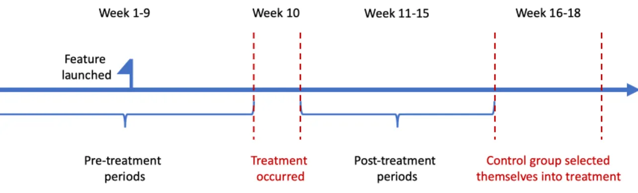
Figure 2-1: Timeline of sampling scheme
who made modifications to their interest categories with more than 10 opt-ins in one time period, week 10. After comparing the user activity measures, we find that there are huge difference between those who have made changes to interest categories, and those who had never made any changes. We decided to sample the control group from those who’ve also made their first changes to their interest categories, but just at later time, in the hope that these two groups will be more similar, or at least there could be fewer unobservable factors that determine their differences. The control group are those who modified their interest categories with more than 10 opt-ins 5 weeks later than the treatment group from week 16 to week 18. We collect these users’ demographic and behavioral data for 15 weeks from March to June. The first 9 weeks are the pre-treatment periods, in which both treatment and control had not stated their interest by making changes to their interest categories. The 10𝑡ℎ
week is the treatment occurring period, during which the treatment group users gradually made their first time changes to their interest categories. And we also kept a record of their data for another 5 weeks after this, to observe the immediate short run effect and relatively long run effect.
We consider multiple performance metrics as the outcome variables to measure the users’ app and ad engagement. The variables include the total amount of time each user views the in-app advertisement every period, the total number of ads that each user views the in-app advertisement every period, the average length of time the user views each advertisement during each period conditioning on the user remains to be a weekly active user, the number of app opens, the total amount of time that user uses the app, etc.
We include controls of user demographics, e.g., age group, gender, country, tenure, etc. Due to the fact that some users might randomly fill in an age that is not their true age, the firm also uses machine learning algorithms and social network data to infer the users’ true age. In our analysis, we will be using the inferred age groups provided by the firm. We also include user’s activity measure as our covariates, such as the number of application opens within the period, the number of sessions, the number of views, the total time spent on the app, the number of friends etc. Lastly, we include app system performance data like network speed, swipe latency and how long it takes for the system to successfully make a post, because these variables might also affect users’ willingness to use the app.
2.3
Data Summary
We conduct covariate summary of some covariates in our estimation model. We treat the first 8 covariates like gender, age, phone operation system, tenure duration as time invariant variables. These covariates either are very unlikely to vary within our analysis duration like gender and age groups, or the change is completely predictable like tenure, such that including the variable in each period will not add any additional information to our analysis. Overall, the statistics of these binary variables are generally consistent for the treatment and control groups. The patterns are that there are more female users than male users. Less than half of the users in the sample are Android users.
The other covariates are time-varying covariates and performance metrics in the first two pre-treatment periods. We find that basically all covariates related to user’s activity level are consistently higher in treatment group compared to the control group, such as ad view time and counts, number of app opens, number of app session starts and ends, number of views, total amount of time spent with the app, etc. In Fig 3-1, we also plot some outcome metrics (on a relative scale) that we measure to indicate user’s engagement level with ads, such as total ad view time in the period, ad view count and average ad view time per ad. Same as what we’ve observed in the covariate table, the user’s average engagement level with ads is consistently higher in treatment group than in control group in the pre-treatment periods, as indicated by the left part of the vertical line in each plot. Although the table
only presents summary statistics of the first two periods of the pre-treatment duration. The pattern is consistent across all the nine pre-treatment periods. These all suggest the covariate imbalance, and the necessity to correct for such imbalance.
Chapter 3
Results and Analysis
3.1
Model Identification
Our main identification method is to use difference-in-difference with matching to estimate the average treatment effect on the treated. A simple DID estimator can be estimated by the regression
𝑌𝑖𝑠𝑡 = 𝛾𝑠+ 𝜆𝑡+ 𝛿𝐷𝑠𝑡+ 𝜖𝑖𝑠𝑡
where 𝑖 denotes individual, 𝑠 denotes treatment assignment and 𝑡 denotes time. 𝐷𝑠𝑡 is a
dummy variable that equals one for treatment units 𝑠 = 1 in the post-treatment period (𝑑𝑡 = 1) and is zero otherwise. Our coefficient of interest is 𝛿. Additionally, since we are
also interested in learning how effects change period by period, we have our second model specification
𝑌𝑖𝑠𝑡 = 𝛾𝑠+ 𝜆𝑡+
∑︁
𝑡′∈{post periods}
𝛿𝑡′𝐷𝑠𝑡′ + 𝜖𝑖𝑠𝑡
where 𝐷𝑠𝑡′ are interaction terms between treatment assignment and each post-treatment
period. Our coefficients of interest are 𝛿𝑡′.
The key assumption underlying the validity of diff-in-diff method is the parallel trends in control and treatment groups (Angrist and Pischke 2008). Here we make a plot of the control and treatment group ad engagement behavior before and after the treatment as shown in Fig. 3-1. The vertical line represents the last period (Week 9) of the pre-treatment periods.
All the plots up till the vertical line are pre-treatment data. Although the outcome of the control group is consistently below the treatment group in the pre-treatment periods, they are far from being perfectly parallel. In order to construct a better estimator that fulfills the parallelism assumption, we perform weighting and assign each user a propensity score weight while performing DID estimation. We choose weighting over matching mainly because our sample size is small, and matching generally means discarding some sample points.
Figure 3-1: Original outcome plots without matching. The top two figures are ATT effects and the bottom three figures are ATT on always active users. The vertical line denotes the last pre-treatment period.
We weight each individual user based on all the variables we’ve introduced above including time-varying outcome variables, user activity variables, app performance metrics in all the nine pre-treatment periods as well as time invariant user demographics. We’ve also tried several different weighting methods, such as propensity score weighting (Angrist and Pischke 2008), generalized full weighting (Sävje, Higgins, and Sekhon 2017) and Covariate Balancing
Propensity Score weighting (Imai and Ratkovic 2014). Since our goal of weighting is to achieve parallel pre-treatment trend between the treatment and control groups, we decided that the Covariate Balancing Propensity Score weighting (CBPS) gives the best result, as shown in Fig. 3-2. The CBPS method makes use of the propensity score as both a covariate balancing score and the conditional probability of treatment assignment, and it is robust to mild misspecification of the parametric propensity score function (Imai and Ratkovic 2014). The key assumption is that no unobservable characteristics are correlated with both selection into treatment and outcomes of interest. The red line indicates the treatment group and the blue line denotes the control group. The 95% confidence bands are also plotted in the figures with corresponding colors. The top two figures are the plots of the entire sample. The bottom three figures are the plots of those who remained weekly actively throughout the entire period. Simply through eyeballing, we could see that the two groups are almost perfectly overlapping in the pre-treatment periods including both the sample means and confidence bands. Compared to Fig. 3-1, this looks much better in terms of achieving parallelism. Hence we will be using DID weighted by CBPS weighting method.
Another identification strategy that we’ve employed is that instead of having people who’ve never changed their interest categories as control, we choose the control group from people who eventually still changed their interest categories, just at a later time compared to treatment group. As explained in sampling scheme section, this serves to minimize the original observable and unobservable differences between the treatment and control group. Accordingly, we are unable to estimate the average treatment effect (ATE) on the whole population, because the sample was not drawn from the whole population, but a distinct subgroup of the population. We are able to identify the average treatment effect on the treated (ATT), and fortunately, ATT is also important for the firm’s policy making. Since there is no way to force a person who does not want to modify their interest categories to make changes, the effect of those who would willingly modify interest categories is what we ultimately care about.
To sum up, the three identification strategies that we employ include 1) selecting control group from those who were eventually still treated to mitigate the unobserved heterogeneity between treatment and control groups, 2) covariate balancing propensity score weighting by
Figure 3-2: Covariate Balance Propensity Score weighted outcome variables in each time period. The two figures on the top are ATT effects and the three figures on the bottom are ATT on always active users.
assuming selection on observables, and 3) difference-in-difference.
3.2
Results
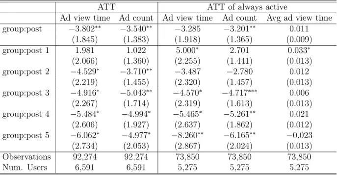
Table 3.1 presents the results of our DID estimation weighted by Covariate Balancing Propen-sity Score. ATT and ATT of always active users are the effects that we are estimating here. Below are the explanation of what each outcome variable means:
• Ad view time: the total length of time each person views the advertisement within a period, i.e., a week. The units are in seconds.
• Ad view count: the total number of advertisements each person views while using the app within a period. In our following research, we will be using ad view count as
a proxy for users’ engagement with organic content. The reason we could do so is that the frequency of assigning an advertising slot for each user is generally fixed, and changing interest categories do not affect such frequency.
• Mean view time: the average length of time in seconds each person views each ad within a week. It is calculated by ad view time for user 𝑖
ad view count for user 𝑖. The mean ad view time per ad
is considered as a proxy for users’ interest in advertising.
In Table 3.1, the first estimator "group:post" is overall treatment effect obtained from our first model specification. The remaining estimators "group:post #" are the effects in each post-treatment period as obtained from the second model specification. The standard errors that we presented in the table are cluster robust standard errors obtained by cluster boot-strapping because we want to have estimates robust to each individual’s heteroskedasticity and meanwhile we want to keep the serial correlation of observations for each individual. We also use the number of * to indicate the p-values of the estimators.
ATT ATT of always active
Ad view time Ad count Ad view time Ad count Avg ad view time group:post −3.802** −3.540** −3.285 −3.201** 0.011 (1.845) (1.383) (1.918) (1.365) (0.009) group:post 1 1.981 1.022 5.000* 2.701 0.033* (2.066) (1.360) (2.255) (1.441) (0.013) group:post 2 −4.529* −3.710** −3.487 −2.780 0.012 (2.219) (1.455) (2.320) (1.457) (0.013) group:post 3 −4.916* −5.043** −4.570* −4.717*** 0.006 (2.267) (1.714) (2.319) (1.613) (0.013) group:post 4 −5.484* −4.994* −5.465* −5.261** 0.021 (2.606) (1.927) (2.637) (1.862) (0.012) group:post 5 −6.062* −4.977* −8.260** −6.165** −0.023 (2.734) (2.053) (2.867) (2.024) (0.013) Observations 92,274 92,274 73,850 73,850 73,850 Num. Users 6,591 6,591 5,275 5,275 5,275 ***𝑝 < 0.001,**𝑝 < 0.01,*𝑝 < 0.05
Table 3.1: Covariate Balance Propensity Score Weighted DID Estimates
There is an important difference I need to clarify in terms of the sample that we’ve used to estimate DID effect on the total ad view time and ad view count per user on the left
side, vs. the two together with the mean ad view time per ad per user on the right side of the table. The left two columns correspond to the two top plots in Fig. 3-2. When a user does not see any ads within a period, we consider both the total ad view time and count to be 0. The total number of treatment group is around one third of the control group. However, we are not able to calculate the average ad view time for some users in the entire sample, because the denominator (ad view count) could be 0. Therefore, for the right three outcome variables which correspond to the bottom three plots in Fig. 3-2, we consider the treatment effect on the always active users. Always active users refers to the group of users who always remain to be weekly active. Here we define weekly active as the users who see at least one ad in the app each week. In this case, the total number of treatment group and control group are both reduced. Overall, among treatment group, 79% of users remain to be weekly active in the all post-treatment period. In comparison, 81% of control users remain weekly active. We conducted a proportion test of the two retention rates, and the p-value is 0.051, which we consider weakly significant difference between the two retention rates. The difference confirms we cannot assume user dropping out as a random event independent of the treatment. This result is consistent with the overall negative impacts on the total ad view time and count which we will discuss further in the following paragraph. One clarification of our definition of always active users is that this is based on observed behavior, so we should not consider it as a subgroup under principal stratification.
The overall effect on mean ad view time per ad for each user is insignificant. If we break them down period by period, then we find there is a significant positive effect in the first period after the treatment group users made changes to their interest categories. Such effects quickly diminish and become insignificant for all the remaining periods. This means for users who remain active throughout the 15 weeks, those who were shown ads based on their stated interest categories show slightly higher interest in ads compared to those who were shown ads based on firm’s inferred interest categories, within one week after users disclose their interest to the firm. However, after one week the two groups of users show similar level of interest towards ads.
In terms of total ad view time and ad view count, the estimates are very consistent with the trend plots that we’ve included in Fig. 3-2. The overall effects are generally significantly
negative in terms of ad view time and ad view count for both ATT and ATT on always active users. In the first week right after the treatment occurred, the effects for both are insignificant. Starting from post period 2, both estimates went significantly negative for ATT, and the effect of ad view time and count becomes increasingly more negative throughout the periods. This means that users’ engagement with organic content declines with time. As for ATT of those who remain weekly active throughout the time, the estimates are negative but fewer are significant. Comparing the two sets of estimates, we observe that the effects on ATT vs. ATT of always active users do not vary by a lot but ATT has more significance in estimates, probably due to the larger sample size in this case. Hence in our future analysis, we would use ATT estimates whenever we could. Only when ATT is not feasible, such as mean ad view time which requires division and denominator cannot be 0, then we would present estimates of ATT of always active users. Overall, in the relatively long term, there seemed to be significantly negative effects on both ad counts and ad view time, which we consider as a proxy of user’s overall app engagement.
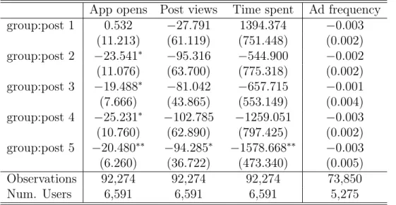
We want to confirm that total ad view counts could be seen as such a proxy. The main concern is that although advertising slot is fixed, when no advertisement could serve as a candidate to this slot, it will appear as a blank page. It is possible that change interest categories would affect the number of ad candidate this user has. Therefore, to confirm the validity of our approximation, specifically to confirm that the number of ad candidates would not be affected significantly, in Table 3.2 last column, we perform the same weighted DID using ad frequency as the outcome metric. The ad frequency is defined by the total number of actual ads a user sees within a week divided by the total number of organic contents a user sees within a week. Given the relatively large standard errors, we observe no significant effects at all. It confirms the fact that users making changes to their interest categories has no effect on ads frequency at all. Moreover, in column (1) to (3), we use some other organic activity related variable as our outcome metrics, such as the number of app opens, the total number of views and the total amount of time spent using the app. We observe that the overall patterns of these three estimates are consistent with the total ad view time and counts, as they are all positive at the beginning, and quickly become negative in the relatively long term. This supports our analysis that takes user’s ad view counts as a proxy
of user engagement with the app.
App opens Post views Time spent Ad frequency group:post 1 0.532 −27.791 1394.374 −0.003 (11.213) (61.119) (751.448) (0.002) group:post 2 −23.541* −95.316 −544.900 −0.002 (11.076) (63.700) (775.318) (0.002) group:post 3 −19.488* −81.042 −657.715 −0.001 (7.666) (43.865) (553.149) (0.004) group:post 4 −25.231* −102.785 −1259.051 −0.003 (10.760) (62.890) (797.425) (0.002) group:post 5 −20.480** −94.285* −1578.668** −0.003 (6.260) (36.722) (473.340) (0.005) Observations 92,274 92,274 92,274 73,850 Num. Users 6,591 6,591 6,591 5,275 ***𝑝 < 0.001,**𝑝 < 0.01,*𝑝 < 0.05
Table 3.2: DID estimates on app usage outcome variables
We also test whether the treatment exerts any impact on the smoothness of app usage experience, such as post delay and swipe latency as shown in Table A.1 in Appendix. We observe that the treatment does not have any effect in these aspects based on the results.
3.3
Robustness Checks
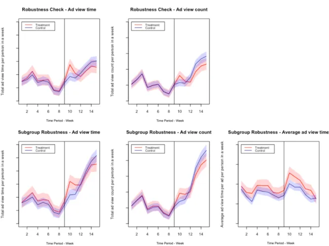
In this subsection, we mainly want to assess the robustness of our proposed identification methodology. We first conducted a placebo test. Since there are a total of 9 pre-treatment periods, instead of matching data on all the 9 pre-treatment periods, we construct weights from the first 7 pre-treatment periods by assuming the treatment occurs right after Week 7 and before Week 8. We tested whether there is any treatment effect in pre-treatment period 8 and 9, using period 7 as the baseline to take difference to construct weighted DID estimator.
Table 3.3 presents the results of this placebo test. Placebo Post 1 estimate indicates the weighted difference between baseline period and period 8, which is 2 periods before the actual treatment occurs but in this placebo test we assume the treatment starts in this period, and Placebo Post 2 estimates the weighted difference between baseline period and
Ad view time Ad view count Mean view time
Placebo Post 1 (Week 8) 0.267 0.624 0.003
(1.507) (0.928) (0.015)
Placebo Post 2 (Week 9) 2.027 1.163 0.004
(1.805) (1.103) (0.015)
Observations 92,274 92,274 73,850
Num. Users 6591 6591 5275
***𝑝 < 0.001,**𝑝 < 0.01,*𝑝 < 0.05
Table 3.3: Placebo test supposing treatment takes place after week 7
period 9, which is one period prior to the actual treatment but here we assume it’s the second period since the treatment starts. All the p-values are way larger than the significance level 0.05, confirming the validity of our matching.
Another way to assess our selection-on-observable, i.e., whether the covariates that we’ve included in our data are good enough to represent the difference between treatment and con-trol group endogenous difference, is by matching the pre-treatment periods without matching their outcome metrics, in this case the total ad view time, ad view count and mean ad view. Then we compare whether the matching without the outcome metrics can produce a weighted control group as similar as the treatment group in terms of the outcome metrics. If so, then we could get another confirmation that our selection on observables approach is good enough to represent the difference between the two groups. Based on Fig. 3-3, the ATT of ad view count has been matched perfectly. Total ad view time is not matched as well as ad count but still reasonably well.
We also want to assess the robustness of DID strategy by conducting DID without weight-ing, and the results are shown in Table 3.4. The overall patterns are consistent with the what we’ve obtained with weighted DID, with estimates initially positive and later with ad view time and count being significantly negative, but mean ad view time per ad becomes insignificant. This shows the robustness of DID strategy in our case regardless of whether we perform weighting and what techniques we use.
Moreover, we perform causality test that tests for anticipatory effect by including the interaction terms between treatment assignment and pre-treatment periods. We find there
Figure 3-3: Matching without outcome variables. The top two figures are ATT effects and the bottom three figures are ATT on always active users.
is no significant anticipatory effect on dummies for future policy changes. 𝑌𝑖𝑠𝑡= 𝛾𝑠+ 𝜆𝑡+ ∑︁ 𝑝∈{post periods} 𝛿𝑝𝐷𝑠,𝑝+ ∑︁ 𝑝∈{pre periods} 𝛿𝑞𝐷𝑠,𝑞+ 𝜖𝑖𝑠𝑡
Finally, we try adding group-specific time trends that allows the treatment and control groups to follow different trends. We find the estimated effects of interest are generally unchanged by the inclusion of these trends as shown in Table A.4 in Appendix.
3.4
Heterogeneous Effects
Heterogeneous effects are also an important guide to inform us whom might behave differently and how different. In the section, we discuss the heterogeneity based on user behavior such
Ad view time Ad count Mean view time group:post −2.343 −2.269 0.002 (1.729) (1.280) (0.008) group:post 1 3.499 2.172 0.025 (1.933) (1.258) (0.013) group:post 2 −2.722 −2.072 −0.001 (2.001) (1.320) (0.013) group:post 3 −3.514 −3.787* −0.0003 (2.130) (1.580) (0.013) group:post 4 −3.751 −3.664* 0.015 (2.450) (1.791) (0.012) group:post 5 −5.229* −3.997* −0.031* (2.595) (1.922) (0.012) Observations 92,274 92,274 73,850 Num. Users 3,286 3,286 2,625 ***𝑝 < 0.001,**𝑝 < 0.01,*𝑝 < 0.05
Table 3.4: DID estimates without weighting
as engagement level and tenure duration, user demographics such as gender. Due to the small sample size, we do not divide the sample into more than 2 groups each time. When we are grouping people based on a continuous covariate, we always try to set the cutoff around the median so that the sample size in each group will be close.
Female Users Male Users
Ad view time Ad count Avg view time Ad view time Ad count Avg view time
group:post −5.386* −4.585** 0.009 0.645 −0.610 0.017 (2.145) (1.635) (0.010) (3.584) (2.458) (0.017) group:post 1 −0.690 −0.420 0.020 9.493* 5.079* 0.069* (2.354) (1.588) (0.016) (4.118) (2.534) (0.027) group:post 2 −6.578* −5.323** 0.012 1.217 0.817 0.013 (2.559) (1.688) (0.015) (4.662) (2.931) (0.028) group:post 3 −5.866* −5.984** 0.008 −2.251 −2.405 −0.0004 (2.617) (1.962) (0.014) (4.398) (2.872) (0.026) group:post 4 −7.279* −6.030** 0.019 −0.444 −2.088 0.025 (3.011) (2.317) (0.015) (5.049) (3.473) (0.025) group:post 5 −6.518 −5.167* −0.023 −4.789 −4.452 −0.023 (3.226) (2.524) (0.014) (4.981) (3.541) (0.026) Num. Obs. 68,726 68,726 55,244 23,548 23,548 18,606 Num. Users 4,909 4,909 3,946 1,682 1,682 1,329 ***𝑝 < 0.001,**𝑝 < 0.01,*𝑝 < 0.05
Table 3.5: Weighted DID for Female vs. Male Users
sample size is much smaller than the female user, there is not much significance observed from the male user group. Surprisingly, in post 1 period in Table 3.5, the mean ad view time for male users, despite the small sample size, are significantly positive. Across the entire duration, male users tend to have more positive responses compared to female users. This probably has some engineering implications. Due to the relatively smaller size of male users, the ad targeting based on firm inferred interest is not as good as that of female users. Thus once male users have the option to state their preferences, we see a significant improvement in their interest in ads at least in the short run. The engineering implication is that the algorithm needs to be more considerate of gender difference when recommending ads to users.
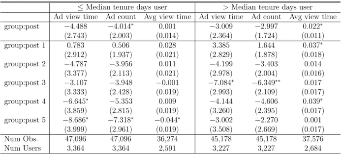
Next we explore the impact on newer users vs. users with longer tenure. Therefore we set the cutoff between the two heterogeneous groups to be the median tenure days in Table 3.6. The interesting results about this part of heterogeneity is that the longer tenure users show more interest in ads after the treatment, in terms of both the overall effects and period by period effects. On the contrary, the mean ad view time for user with shorter tenure has no significantly positive effects at all.
≤Median tenure days user >Median tenure days user
Ad view time Ad count Avg view time Ad view time Ad count Avg view time
group:post −4.488 −4.014* 0.001 −3.009 −2.997 0.022* (2.743) (2.003) (0.014) (2.364) (1.724) (0.011) group:post 1 0.783 0.506 0.028 3.385 1.644 0.037* (2.912) (1.937) (0.021) (2.829) (1.878) (0.018) group:post 2 −4.787 −3.956 0.011 −4.199 −3.403 0.014 (3.377) (2.113) (0.021) (2.978) (2.004) (0.016) group:post 3 −3.107 −3.948 −0.001 −7.084* −6.349** 0.017 (3.333) (2.428) (0.019) (2.993) (2.109) (0.017) group:post 4 −6.645* −5.353 0.009 −4.144 −4.606 0.039* (3.859) (2.815) (0.019) (3.260) (2.395) (0.017) group:post 5 −8.686* −7.318* −0.044* −3.002 −2.270 0.001 (3.999) (2.961) (0.019) (3.508) (2.669) (0.017) Num Obs. 47,096 47,096 36,274 45,178 45,178 37,576 Num Users 3,364 3,364 2,591 3,227 3,227 2,684 ***𝑝 < 0.001,**𝑝 < 0.01,*𝑝 < 0.05
Table 3.6: Weighted DID effects on users with short vs. long tenure duration
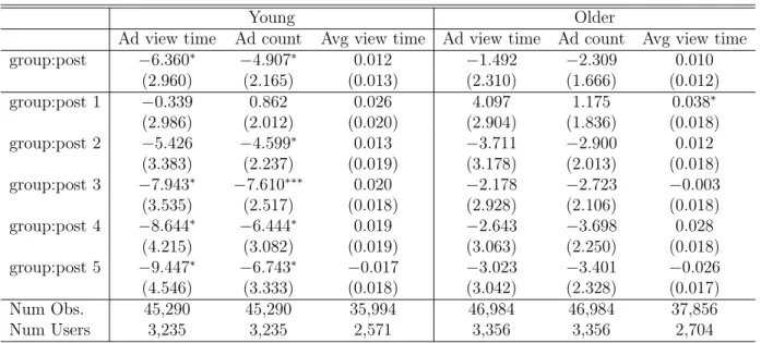
Finally we find there is also heterogeneous effects based on the users’ inferred age as shown in Table 3.7. In our sample, around 50% users are inferred as young people, and the
remaining 50% are inferred as relatively older adults. Overall, younger users have a more negative reaction after the treatment compared to relatively older adult users.
Young Older
Ad view time Ad count Avg view time Ad view time Ad count Avg view time
group:post −6.360* −4.907* 0.012 −1.492 −2.309 0.010 (2.960) (2.165) (0.013) (2.310) (1.666) (0.012) group:post 1 −0.339 0.862 0.026 4.097 1.175 0.038* (2.986) (2.012) (0.020) (2.904) (1.836) (0.018) group:post 2 −5.426 −4.599* 0.013 −3.711 −2.900 0.012 (3.383) (2.237) (0.019) (3.178) (2.013) (0.018) group:post 3 −7.943* −7.610*** 0.020 −2.178 −2.723 −0.003 (3.535) (2.517) (0.018) (2.928) (2.106) (0.018) group:post 4 −8.644* −6.444* 0.019 −2.643 −3.698 0.028 (4.215) (3.082) (0.019) (3.063) (2.250) (0.018) group:post 5 −9.447* −6.743* −0.017 −3.023 −3.401 −0.026 (4.546) (3.333) (0.018) (3.042) (2.328) (0.017) Num Obs. 45,290 45,290 35,994 46,984 46,984 37,856 Num Users 3,235 3,235 2,571 3,356 3,356 2,704 ***𝑝 < 0.001,**𝑝 < 0.01,*𝑝 < 0.05
Table 3.7: Weighted DID on young users vs. older users based on inferred age
In addition, we’ve also tried exploring the heterogeneous effects based on users’ activity level in Table A.2 and the app performance, e.g. post delay in Table A.3 in the Appendix, but we do not observe obvious differences between users.
Chapter 4
Discussions and Conclusion
4.1
Causal Discussion
4.1.1
Direct Treatment Period
In our DID analysis, we’ve discard all the results from week 10, because it is the period when the treatment is occurring, i.e., it is an ongoing process that treatment group users select themselves into the treatment. In this period, we observe that the treatment group has a significantly higher interest in ads as illustrated by average time viewing each ad and significantly higher user activity level, as illustrated by the metrics like time spent using the app, number of app opens, number of ads displayed given the ad frequency remains unchanged, etc. As shown in Figure. 4-1, we cannot tell whether the treatment causes higher user engagement with the app, or whether it’s higher user engagement that makes users find out the feature and then select themselves into the treatment group during this period. Additionally, we are not able to distinguish how much impact attributes to pre-treatmentand how much is the post-treatment effect. Therefore, we choose not to interpret too much about the results in this period.
Moreover, research has shown that activity bias could pose an issue in causal identification (Lewis, Rao, and Reiley 2011). In our case, activity bias arises because users’ app use activity might be correlated with finding the interest category feature. In order to mitigate such bias, we’ve adopted two strategies. First, we choose not to interpret the post 0 period estimates
Figure 4-1: Post-treatment period 0 directed causal graph
as causal effects, because post 0 period include the immediately post-treatment behavior of most treatment users. Second, we perform analysis on a weekly basis not on a daily basis. The research so far has only found such activity bias on the given day of the treatment (Lewis, Rao, and Reiley 2011). We hope with more days included in each data point, the outcome of interest data should be relatively more stable.
4.1.2
Possible Mechanisms
Based on post 1 period DID estimates we could still conclude in the very short run, there is a weakly significant increase in user’s average interest in ads for users who’ve stated their interest categories, compared to users who are targeted based on firm inferred interest. This is a positive signal, suggesting that users are getting more interested in ads after the firm adopts their stated interest in ad targeting.
In the long term, however, there is no significant difference between treatment and control groups in terms of the average time each user views each ad, but there is significantly negative effects in terms of the overall user activity/user app engagement, as reflected by the outcome variables like the ad count, total time spent using the app, etc. in Table 3.1 and Table 3.2. This could be attributed to that the user profile information is shared for both ad targeting and content recommendation purposes.
A possible reason is that users select their interests based on what advertising content they’d prefer to see, and what they’d like to see for ads are different from what they’d like to see for organic contents. For example, a user who likes to watch organic videos of luxury cars does not necessarily want to purchase a luxury car. Hence the change in recommended contents reduces their interest in app content, subsequently the overall app usage.
to select very specific interest categories when they have the chance to modify their interest categories, and there is a limited number of organic contents and ads falling into these specific categories. Given users see far more organic content than ads, users are more likely to see similar or repeating content compared to ads, and hence they tend to get tired of contents faster than ads.
Furthermore, since it is a social app firm, the increasingly negative effects in the later period could be partially attributed to the network spillover effects. The reduced app en-gagement of one user could easily exerts a negative effect on other users’ app enen-gagement level.
4.2
Managerial Implications
The adoption of user stated interest categories seems to create a tension between long term vs. short term effects, as well as ad targeting vs. organic content recommendation. Although it does seem to exert a short run positive effect in raising people’s average interest in ads, the long term negative effect on people’s app engagement seems to be far more detrimental, offsetting the initial benefits. Since this feature is mandated by the privacy regulations, one possible managerial strategy that could prevent such negative effects is that firms might want to create two user profiles for ad targeting and content recommendation purposes respectively. However, this might not be always practical. Firms could also consider how to incorporate such difference in their organic content recommendation and ad targeting algorithms.
Another managerial implication is drawn based on the fact that users who have volun-tarily made changes to their interest categories in fact have increased interest in advertising. Therefore, the firm could consider sending frequent reminder to users who have already made changes to their interest categories to update their interest.
4.3
Conclusion
In this paper, our main goal is to assess the effect of ad targeting using user stated interest, compared to using firm’s inferred interest on user’s ad engagement. We find that overall there is no significant effect. However, immediately after users stated their interest by modifying their interest categories in the app, users’ average interest in ads does improve a little, although such effect quickly diminishes. In terms of user’s engagement with the app, we used the number of ads seen as a proxy. Results obtained from such a proxy is further confirmed by other proxies such as the number of app opens, and time spent using the app, etc. Initially there is no significant effects. In the longer term, the proxies for user engagement all show negative signs and many have remained significant in all the remaining periods. We hypothesize the reason to be that the firm used this updated user profile for both ad targeting and content recommendation, and users like what’s recommended for ads but dislike what’s recommended for organic content after they modified their interest categories in their profile. This calls for the attention on the difference between organic contents and advertisements targeting that requires further research to investigate. Future research could also provide more evidence or theoretical support on our hypothesized mechanisms.
Based on this finding, we also identify another area for future work is to theorize and explore how to induce at least partial truth telling from more users, and what mechanism encourages more truth revelation, when users are explicitly informed that the user profile is for both organic content recommendation and ad targeting. Users might have conflicted motivation in this case: on one hand, they do not want to be targeted with ads and thus feel reluctant to reveal their true information; on the other hand, they’d like to see the organic contents match their preferences better and thus have incentive to reveal some information. We’ve also explored the heterogeneous effects. Specifically, we find that users with long tenure duration tend to be more interested in ads and the increase in interest lasts for a longer time compared to newer users after stating interest. Demographically, we find that male users exhibited more positive reactions in terms of ad interest after they stated their interest, and younger users exhibit more negative reactions in terms of app engagement.
data granularity. Since this is an observational study, there might be some other endogenous issues that we have not accounted for. Our result analysis could benefit a lot if we could have more information on the specific ads that users saw each time, and the specific interest categories that users have made changes to. Another limitation is that throughout the entire analysis, we have not accounted for the magnitude of the network spillover effects, that might exist in the effect on user app engagement level based on the nature of the social app.
Appendix A
Additional Tables
post delay swipe latency
group:post 1 2.776 -1.002 (2.299) (1.059) group:post 2 -0.730 -1.074 (1.998) (0.948) group:post 3 6.517 1.828 (4.561) (2.868) group:post 4 -1.086 -1.584 (2.089) (1.176) group:post 5 -0.184 -0.728 (2.159) (1.038) Observations 73,850 73,850 Num. Users 5,275 5,275 ***𝑝 < 0.001,**𝑝 < 0.01,*𝑝 < 0.05
≤median weekly app opens >median weekly app opens Ad view time Ad count Mean view time Ad view time Ad count Mean view time
group:post 1 4.088 1.592 0.047* 0.134 0.493 0.020 (2.563) (1.514) (0.023) (3.129) (2.136) (0.015) group:post 2 −3.134 −2.263 −0.002 −5.857 −5.085* 0.025 (2.549) (1.573) (0.022) (3.564) (2.359) (0.017) group:post 3 −4.070 −3.880* 0.004 −6.126 −6.574* 0.007 (2.748) (1.713) (0.022) (3.347) (2.604) (0.014) group:post 4 −3.683 −3.202 0.020 −7.575 −7.119* 0.020 (2.857) (1.780) (0.021) (4.017) (3.107) (0.015) group:post 5 −8.536** −5.122** −0.048** −4.585 −5.538 −0.003 (2.794) (1.859) (0.020) (4.335) (3.338) (0.016) Observations 46,004 46,004 36,750 46,270 46,270 37,100 Num. Users 3,286 3,286 2,625 3,305 3,305 2,650 ***𝑝 < 0.001,**𝑝 < 0.01,*𝑝 < 0.05
Table A.2: Weight DID on less active vs. more active users
≤median delay >median delay
ad view time ad count mean ad view ad view time ad count mean ad view
group:post 1 -0.494 0.145 0.028 4.069 1.602 0.032 (2.909) (1.838) (0.023) (3.235) (2.130) (0.023) group:post 2 −6.277* -3.989 0.008 -3.154 -3.721 0.010 (3.142) (2.057) (0.023) (3.368) (2.180) (0.023) group:post 3 −6.867* −5.290* 0.002 -3.349 -5.065 0.004 (3.282) (2.263) (0.024) (3.640) (2.652) (0.022) group:post 4 -5.954 -4.676 0.019 -5.370 -5.583 0.018 (3.832) (2.697) (0.023) (4.086) (3.062) (0.023) group:post 5 -4.566 -2.975 -0.024 -7.904 −7.232* -0.027 (4.050) (2.878) (0.022) (4.397) (3.311) (0.024) Observations 46,130 46,130 36,960 46,144 46,144 36,890 Num. Users 3,295 3,295 2,640 3,296 3,296 2,635 ***𝑝 < 0.001,**𝑝 < 0.01,*𝑝 < 0.05
Table A.3: Weighted DID based on post delay
Ad view time Ad count Mean ad view time group:post (𝛿) −5.730 −4.732* −0.021
(3.007) (2.194) (0.018)
Observations 92,274 92,274 73,850
Num. Users 6,591 6,591 5,275
***𝑝 < 0.001,**𝑝 < 0.01,*𝑝 < 0.05
Bibliography
Ahmed, Amr et al. (2011). “Scalable distributed inference of dynamic user interests for behavioral targeting”. In: Proceedings of the 17th ACM SIGKDD international conference on Knowledge discovery and data mining. ACM, pp. 114–122.
Aly, Mohamed et al. (2012). “Web-scale user modeling for targeting”. In: Proceedings of the 21st international conference on world wide web. ACM, pp. 3–12.
Angrist, Joshua D and Jörn-Steffen Pischke (2008). Mostly harmless econometrics: An em-piricist’s companion. Princeton university press.
Beales, Howard (2010). “The value of behavioral targeting”. In: Network Advertising Initiative 1.
Bleier, Alexander and Maik Eisenbeiss (2015). “Personalized online advertising effectiveness: The interplay of what, when, and where”. In: Marketing Science 34.5, pp. 669–688. Boerman, Sophie C, Sanne Kruikemeier, and Frederik J Zuiderveen Borgesius (2017). “Online
behavioral advertising: A literature review and research agenda”. In: Journal of Adver-tising 46.3, pp. 363–376.
Choi, Hana et al. (2017). “Online display advertising markets: A literature review and future directions”. In: Columbia Business School Research Paper 18-1.
Chung, Christina Yip et al. (Oct. 2010). Model for generating user profiles in a behavioral targeting system. US Patent 7,809,740.
Farahat, Ayman and Michael C Bailey (2012). “How effective is targeted advertising?” In: Proceedings of the 21st international conference on World Wide Web. ACM, pp. 111–120. Goldfarb, Avi and Catherine Tucker (2011a). “Online display advertising: Targeting and
obtrusiveness”. In: Marketing Science 30.3, pp. 389–404.
— (2011b). “Privacy regulation and online advertising”. In: Management science 57.1, pp. 57– 71.
Imai, Kosuke and Marc Ratkovic (2014). “Covariate balancing propensity score”. In: Journal of the Royal Statistical Society: Series B (Statistical Methodology) 76.1, pp. 243–263. Johnson, Garrett, Scott Shriver, and Shaoyin Du (2019). “Consumer privacy choice in online
advertising: Who opts out and at what cost to industry?” In:
Lambrecht, Anja and Catherine Tucker (2013). “When does retargeting work? Information specificity in online advertising”. In: Journal of Marketing Research 50.5, pp. 561–576. Lewis, Randall A, Justin M Rao, and David H Reiley (2011). “Here, there, and everywhere:
correlated online behaviors can lead to overestimates of the effects of advertising”. In: Proceedings of the 20th international conference on World wide web. ACM, pp. 157–166.
Pandey, Sandeep et al. (2011). “Learning to target: what works for behavioral targeting”. In: Proceedings of the 20th ACM international conference on Information and knowledge management. ACM, pp. 1805–1814.
Sävje, Fredrik, Michael J Higgins, and Jasjeet S Sekhon (2017). “Generalized Full Matching”. In: arXiv preprint arXiv:1703.03882.
Trusov, Michael, Liye Ma, and Zainab Jamal (2016). “Crumbs of the cookie: User profiling in customer-base analysis and behavioral targeting”. In: Marketing Science 35.3, pp. 405– 426.
Tucker, Catherine (2012). “The economics of advertising and privacy”. In: International jour-nal of Industrial organization 30.3, pp. 326–329.
— (2014). “Social networks, personalized advertising, and privacy controls”. In: Journal of Marketing Research 51.5, pp. 546–562.