The demand for housing in the United Stated [sic] and West Germany : a discrete choice analysis

by

Axel Boerach-Supan

Diplom-Mathematiker, University of Bonn, West Germany (1.980 )

Submitted to the Department of Economics In Partial Fulfillment of the ReqUirements

For the Degree of

Doctor of Philosophy

at the

Massachusetts Institute of Technology June 1984

@ Axel Boersch-Supan

The author hereby grants to X.l.T. permission to reproduce and to distribute copies of this thesis document in whole or in part.

Signature of Author _{, ' f ' !}< J '

Richard Eckaus

ARC;i~i!VF!.S Gra~ate Registration Officer

MASSACHUseITS 'NSTITUTE ; . OF 1tCHNOLOOY

Certif ied bY

-m.:;;;"..__

--...~--.a.-..-::a..:..---+----'----J..,...-~...ga,;rr;=:~~====~ _

, Daniel L. McFadden Thesis Supervisor Accepted by _ I

f

JUN 1

91984

LIBRARIES ..8: ;,M,

THE DEMAND FOR HOUSING IN THE UNITED STATED AND WEST GERMANY: A DISCRETE CHOICE ANALYSIS

Axel Boersch-Supan

Submitted to the Department of Economics on May 4, 1984 in partial fulfillment of the requirements for the Degree of Doctor of Philosophy at the Massachusetts Institute of Technology

ABSTRACT

This thesis applies discrete choice techniques to an analysis of housing demand in the United States and West Germany. Housing demand comprises the choices of household formation, tenure, type of structure, and size and quality of dwelling. We will focus on peculiarities of housing demand which have found little attention in the otherwise ample literature on housing demand. Usage of similar surveys in the United States and West Germany allow us to make comparisons between the two countries and to identify mechanisms which are concealed by examining only one country.

The multidimensional heterogeneity of housing demand possibilities suggests the usage of discrete choice techniques, in particular hierarchically nested choice models. The theory and estimation of nested multinomial logit models is reviewed &nd extended.

Household formation as a dimension in housing demand renders household based models inappropriate. A model which simultaneously determines headship status and conventional housing demand is

developed and estimated for U. S. data. Simulations mimicking the Experimental Housing Allowance Program underscore the importance of

household formation as a factor in housing demand.

The tenant-1andlord relationship over time is examined. Empirical evidence points to the eXistence of tenure discounts, 1eading to a bias in conventional price specifications0 A microeconomic model highlights the potential misinterpretations in housing market analysis when tenure discounts are disregarded. As illustration, we evaluate the German rent and eviction control legislation.

Finally, we compare housing choices in the United States and West Germany. We apply a common analytical model on comparable data sets to examine the differences in tenure choice and size demand. Using this model, we try to isolate behavioral from institutional differences.

Thesis Supervisor: Dr. Elisabeth and James R.

Daniel McFadden,

Personal Data

Date of Birth: December 28, 1954 (Darmstadt, West Germany) Married to Martina Elisabeth Boerscn-Supan

Academic Education

Vordiplom (Economics), University of Munich, June 1976

Vordiplom (Mathematics), University of Munich, December 1976 Diploro (Mathematics), University of Bonn, March ~980

Academic Appointments

Teaching Assistant (Mathematics), University of Munich, 1977 Research Assistant (Econometrics) for Professor Peter Schoenfeld,

University of Bonn, 1978-1980

Lecturer (Applied Econometrics), University of Bonn, Spring 1980 Research Assistant (Urban Economics and Econometrics), Joint

Center for Urban Stud£es of MIT and Harvard University, 1981-1982

Research Assistant (Econometrics) for Professor Daniel McFadden, Department of Economics, M.l.T., 1982-1983

Teaching Assistant (Graduate Applied Econometrics), Department of Economics, M.l.T., Spring 1984 Honors, Scholarships, and Fellowships

Studienstiftung des Deutschen Volkes, 1972-1982

Scholarship of the Department of Economics, M.l.T. , 1982 Sloan Foundation FellowshiPf 1983

Fellow of the Joint Center for Urban Studies of MIT and Harvard University, 1983-1984

ACKNOWLEDGMENTS

It took a good seventh part of my life so far to fulfill what is

called "the requirements for the degree of Doctor of Philosophy" on the title page of this thesis. Four years of neglecting wife and child, ignoring the amenities of Boston (almost), leaving my home

country with parents and friendse I would not be a proper economist not to ask myself whether i t was worth all the trouble, nor would I deserve the appendage Ph.D. not to take this opportunity to philosophize on what I have learned during this time.

Quite a lot. The benefits outweigh the costs. I learned

~conomics, starting pretty much and frustratingly from scratch, in a pace and intensity which I -- finally enjoyed. It convinced me that my place is in applied economics rather than in abstract mathematics. And I learned to ~ike my profession. Apart from economics, I enjoyed the company of such a variety of interesting fellow students and teachers as i t is only possible in this Cambridqean ivory tower. I am grateful to all my friends for discussions, excursion, and symposiums in which we shared the ups and downs of a great time.

I own many thanks to Dan McFadden, my mentor and thesis advisor, on both accounts. He taught me the art of combining solid and well-founded econometrics with the interest in sUbstantive but less palpable since real life issues. And he taught me where to eat the best Peking Duck in town. He contributed essentially to my positive

supported by word and deed our sometimes shaky two career plus child enterprise.

The four years of M.I.T. life were four years living in a new

country.

This was an exciting and mind-opening experience which I do

not want to miss. I am grateful to the Studienstiftung in West

Germany for providing the incentive to sail out to the New World and the generous financial support which made this possible without going through the stage of a dishwasher.

Large benefits do not come without costs. And the costs were borne not only by myself. It is a good and meaningful tradition to dedicate a thesis to the parents. I do this with pleasure and

thankfulness. My parents put me on the road I am now pursuinq, and

always supported me with encouragement even when they had to bear most

of the burden when I left Germany four years ago to go through yet

another study.

The cost were large for my wife as well. What a time! We left

our country, married, got our first child -- all this mixed With constant fickleness about exams, night-long glare at a computer terminal, and the final frenzy to get this thesis finishe~. It is a wonder that she still talks to me. Believe me, I am grateful for such

Finally, these acknowledgments must include all those who oontributed to this thesis by commenting on earlier drafts when the work was still in the snips and thoughts stage. Among those are Jerry Rothenberg and Bill Wheaton in my thesis committee, Wolfgang Eckart and Konrad Stahl in Dortmund, John Pitkin at the Joint Center, and Ray Struyk at the Urban Institute. The Ifo-Institut fuer Wirtschaftsforschung in Munich granted permission to quote from an unpublished interim report and supported the German part of my research.

The work was exciting and rewarding, but i t was the acquaintance with and the support of so many people which made this time worth a considerable part of my life.

1. Chapter One: Introduction and Survey

1.1 SUbstantive Issues 1.2 Methodological Issues 1.3 Organization of the Thesis

2. Chapter Two: The Basic Tool: Nested Multinomial Logit

Demand Functions

2.1 Introduction: Discrete Choice Description of Housing Demand

2.2 Random Utility Maximization and Hierarchical Choice

2e2.1 Microeconomic Theory

2.2.2 Functional Specification of Choice Probabilities

2.2.3 Relation Dissimilarity Parameters and RUM

203 Estimation Techniques

2.3.1 Econometric Theory and Numerical Analysis 2.3.2 Elasticities and Goodness-of-Fit Measures 2.3.3 Aggregate Probability Shares

2.3.4 Choice Based Sampling

2~4 Conclusions 2.5 Footnotes

3. Chapter Three: The Influence of Household Formation on Housing Demand

3.1 Introduction: Review of Earlier Approaches 3.2 Household Decomposition into Nuclei

3.3 Specification of Decision Tree and Variables

3e4 Baseline Estimates

3.5 A Housing Allowance Experiment 3.6 Tax Sirnulatio~s

3.6.1 Cutting the Local Property Tax in One Half

3.6.2 Making the Federal Income Tax Less Progressive

3.7 Conclusions 3.8 Footnotes

4. Chapter Four: Dynamic Aspects in the Housing Market Equilibrium 4.1 Introduction:

Market Imperfections and Government Intervention

4~2 Empirical Evidence on Price Dispersion 4.2.1 Tenure Discounts

4.2.2 Landlord Characteristics and Search 4.3 Rent and Eviction Control in West Germany

4.4 A Microeconomic Model of Tenant-Landlord Relations

4.4.1 The Landlord 4.4.2 The Tenant

4.4.3 Steady State Market Equilibrium

4.5 Rent and Eviction Control with Tenure Discounts Present 4.6 Conclusions

5. Chapter Five: An Analytic Comparison of Housing Demand Decisions In the United States and West Germany

5.1 5.2 5.3 5.4 5.5 5.6 5.7 5.8 5.9 5.10

Introduction: Idea and Scope of an Analytic Comparison A Brief Descriptive Comparison

Tax Treatment of Owner Occupancy in the Two Countries Specification of the Demand Equations

Hedonic Price Indices 5.5.1 United states 5.5.2 West Germany 5.5.3 Comparison

Permanent Income Estimate~

5.6.1 United States 5.6.2 West Germany 5.6.3 Comparison

Estimation of the Demand Equations

5.7.1 Pooled Sample: Optimal Tree Structure 5.7.2 Stratified Sample: Age and Location 5.7.3 Sensitivity AnalySis

Simulations with Tax Laws and Preferences Conclusions

Footnotes

Appendix: FORTRAN Program for Nested MUltinomial Logit Models Bibliography

4: 4-1: 4-2: 4-3: 4-4: 4-5: 4-6: 4-7: 4-8: 4-9: 5-15: 5-16: 5-17: 5-18: 5-19: Table 2-1: Figure 2-2: Figure 2-3: Figure 2-4: Figure 2-5: Chapter 3~ Figure 3-1: Figure 3-2: Tables 3-3f: Table 3-7: Table 3-8: Table 3-9: Table 3-10: Table 3-11: Table 3-12: Table 3-13: Chapter Table Table Table Table Figure Table Table Table Table Chapter 5: Table 5-1: Table 5-2: Table 5-3: Table 5-4: Figure 5-5: Table 5-6: Table 5-7: Table 5-8: Table 5-9: Table 5-10: Table 5-11: Table 5-12: Figure 5-13: Table 5-14: Table Table Table Table Table

Definition of Housing Alternatives

Clusters of Similar Housing Alternatives Decision Trees for Housing Choices

Three Alternatives: Density and Choice Probabilities Choice Probability Preserving Choice Models

Basic Decision Tree

Consolidated Decision Trees for the Different Strata Nested Multinomial Logit Parameter Estimates

Prediction Success Table and Full Elasticity Matrix Own Price and Sum of Income Elasticities

Aggregated Shares: Housing Allowance Experiment Predicted Moves in Response to Housing Allowances Incidence between Jurisdictions and Strata

Aggregated Shares: Local Property Tax Cut Aggregated Shares: Flatter Federal Income Tax

Estimated Tenure Discounts, West Germany, ~978

Estimated Tenure Discounts, United States, ~974-76

Estimated Tenure Discounts, United States, 1976-77 Average Tenure Discounts by Rent Control Status Price Effect of the Tenants' Protection Legislation Discounts for Landlord Present in Building

Discounts for Landlord Private Person Premium for Movers from Outside the SMSA

Specification of Events for Type A Landlord and Tenant

Market Shares of Housing Alternatives

Exogenous Variables: Age, Income, and Prices Stylized Tax Treatment of Homeownership

Tax Savings for a Single-Family Owner-Occupied Home Decision Trees and Housing Alternatives

Hedonic Regression Coefficients: United States Hedonic Regression Coefficients: West Germany Permanent Income Estimation: United States Permanent Income Estimation: West Germany Distribution of Permanent and Current Income

United States, Pooled Sample, WESML-Estimates West Germany, Pooled Sample, WESML-Estimates Chi-Squared Distances

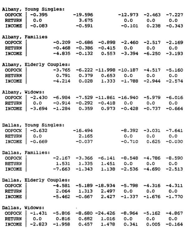
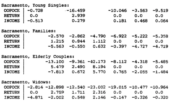
United States, Stratified Sample, Tree T-U-S West Germany, Stratified Sample, Tree T-U-S OWn Price and Sum of Income Elasticities Full Price and Income Elasticity Matrices Sensitivity Analysis

CHAPTER ONE

INTRODUCTION AND SURVEY

10 -***'** ******* ********* *-********* ************* ******** ****** ******** *~**** ******* ****~* ***** *~**** *fe*it** ***fCfl* ****1t* ****** ****** ****** *"**** ****** *************************** ******~=*******ft*********** ***************************

1.1 SUbstantive Issues

This thesis investigates the demand for housing as a heterogeneous commodity. We will focus on the demand side of the housing market in most of our empirical work and restrict the analysis to partial models, that is, on potential demand under perfect elastic supply. This long run analysis is in tune with the use of two large cross-sectional data sets and their interpretation as steady state equilibria: the Annual Housing Survey in the United States and the One Percent Sample in West Germany. The only deviation from our concentration on demand only will be in the theoretical model of the nature of those steady state equilibria.

To capture the heterogeneity of the commodity housing we will introduce a comprehensive notion of what housing demand consists of: i t includes the choices of quality, size, tenure, and headship status. We will not consider choice of location, however, and we will concentrate on large metropolitan areas.

Although housing demand is a well studied field, there are still a host of unresolved sUbstantive issues. Having introduced the notion of the commodity housing as a broad class of different housing categories or alternatives, a general issue is the question of substitutability among these categories. In Joan Robinson9_{s (1933)}

words,

we are looking for the gaps in the chain of SUbstitutes. Do

dwellings for smaller dwellings in

people easily substitute larger

12

-SUbstitutability among housing alternatives change with the life cycle? Are there differences in behavior between the United States

and West Germany?

Furthermore, how does household formation as a dimension of

housing demand fit into the chain of substitutes? Is household

formation responsive to price changes in the rental and owner markets? Does this response depend on the stage in the life cycle or on demographic characteristics?

Apart from interest in the structure of a comprehensive housing demand per se, we might ask ourselves how this structure is reflected in poliCy analysis. The tax codes in both countries are asymmetric in their treatment of owner-occupancy versus rental housing, but i t is not clear whether all of the observed preferences in the tenure choice can be explained by taxes alone. Would a drastic tax change induce a drastic change in the preference for tenure? A comparison and West Germany and the United States seems to be of particular interest due to their very different proportions of owner-occupancy (1978:

u.s.:

65.2 percent, Germany: 36.3 percent). Are there repercussions in the other dimensions of housing choice? What about the response of household formation to changes in the tax code? And, more interesting for the latter dimension, is there a response to direct demand subsidies like housing allowances? Is the Experimental Housing Allowance Program flawed in its complete ignorance of household formation?

A final topic of this thesis and another red thread through the five chapters is the question of what the proper price is for this heterogeneous and durable good. In the last Chapter, we will use hedonic indexes to capture heterogeneity, an at least empirically

resolved issue. However, the durability of housing has implications on intertemporal pricing which are not well understood. Is there

price dispersion in the housing market? How can it be explained? Can different explanations be empirically tested against each other? How does the eXistence of price dispersion affect our knowledge of price responsiveness? And finally, do we have to reevaluate policy analysis in the presence of price dispersion? How does normative analysis of rent and eviction control change in a non-walrasian market With price dispersion?

14

-1.2 Methodological Issues

The comprehensive notion of housing demand as the choice among a collection of heterogeneous alternatives raises many methodological

issues. There is the question of the appropriate functional form for

housing demand equations which include the qualitative and quantitative components of the commodity housing. We will resolve this question in simply dividing the qualitative dimensions into sufficient of discrete categories, and proceed with large discrete choice models.

However, the specification of large discrete choice models is closely related to the question of sUbstitutability among the choices which was raised in the previous section. Is there a feasible compromise between choice models which are easy to compute but impose strict cross-substitution patterns, and choice models which leave freedom for the cross-substitution effects but are computationally intractable? We will show that nested multinomial logit models (McFadden, 1978) constitute such a compromise in housing demand analysis. The unresolved issues at stake is the efficiency loss of the sequential estimation technique and the viability of full information maximum likelihood. A further theoretical issue is

whether the estimation results can be rationalized by a highly structural economic choice model, the random utility hypothesis.

Household formation as a part of housing demand raises the

"household" is endogenous and we face a potential self selection bias in our estimations. How can we resolve this sample selection problem? Is i t possible to avoid a structural model of household formation which is bound to be poorly estimable due to our poor knowledge about this process and will result in a large noise-to-signal ratio? Can we find a reduced form approach with just enough structure to resolve the endoqeneity problem?

A final methodological issue is the handling of price dispersion generated by intertemporal processes when only a single cross section of observations is available. How large is the potential bias in . estimations ignoring price dispersion?

results?

16

-1.3 Organization of the Thesis

The remainder of the thesis is organized in four chapters. The

first of these chapters is devoted to the microeconornic and econometric underpinnings of our basic tool, the nested multinomial logit demand functions. The microeconomic part includes the compatibility of t~ese demand functions with random utility maximization, the econometric part discusses the use of fUll information maximum likelihood estimation.

Chapter Three applies the demand model on the joint choice of household formation, tenure, and size of dwelling to three SMSA's in the United States to answer the question of how price responsive our comprehensive housing demand is. Some microsimulation results illustrate public poliCy implications.

Cnapter Four is a digression on the dynamic nature of the rental housing market. This chapter, mainly microecono~ic theory, is

intended as a motivation and guidance to analyse price dispersion generated by a complicated intertemporal interaction of the demand and supply side.

Finally, Chapter Five applies all the tools we have collected so far on an analytic comparison of housing demand in West Germany and the United States: A common hierarchical choice model for both countries embodies hedonic rent indexes to capture the heteroge~eity

countries.

Each chapter contains an introductory section to present the issues at stake, and a conclusion to summarize the results. An

appendix lists the FORTRAN source of the full information maximum likelihood estimation program for nested multinomial logit models in

18

-CHAPTER TWO

THE BASIC TOOL: NESTED MULTINOMIAL LOGIT DEMAND FUNCTIONS

**************** ********************* ************************* ***********~*************** ********* ****~.**** ~******* ****-***** ***.*~* ********** **~*** ********** ********** ******1r*~* ~"!:~~****** ********** ********** ********** ********** ********** ************~**************** ****************************** ********************~********* ******************************

2.1 Introduction: Discrete Choice Description of Housing Demand

Housing or, more precise, the service stream from a housing unit, is a heterogeneous commodity. Some dimensions, as size or age of structure, are measured on a continuous scale, others, as tenure or

type of structure, are discrete properties. Measuring the volume of housing services as housing expenditure essentially ignores this heterogeneity, and for a large number of policy purposes, the distribution of housing consumpti.on into qualitatively different

categories is of more interest than an aggregate quantitative measure

of housing expenditures alone. The most popUlar example of the interest in qualitative dimensions is the choice between renting and owning, and the response of this tenure choice to federal income tax

treatment. (See Laidler (1969), Rosen (1979), Rosen and Rosen (1980), Henderson and Ioannides (1983).)

We can go one step further: not only the choice of tenure, but also the choices among other continuous or discrete ch·~racteristicsof a housing unit will be affected by taxes and subsidies. Furthermore,

the decision whether to form an autonomous household at all may be

dependent on relative prices and income. ThuS, housing demand

decisions consist of discrete decisionsr e. 9., concerning headship,

tenure, as well as continuous decisions, e. g., size or quality level.

Lee and Trost (1978) and subsequently King (1980) arque that the

tenure choice ~id the choice of size and quality level are made

- 20

-choice is influencing and is in turn influenced by the other two decisions, so that all three choices are made in a joint decision process. This joint decision process constitutes a comprehensive notion of housing demand which will the focus of this thesis.

The econometric theory of joint discrete/continuous models is well studied, and there exist a variety of applications, e. 9. Lee and Trost (1978), King (1980),

or

Dubin and McFadden (1984)e We will not pursue this line of modeling, however, but use consistently a discrete choice framework throughout this work. Sweeney (1974) casts the entire bundle of quality characteristics into discrete categories

so that housing units can be arranged in a commodity hierarchy. We will use a similar discretization of the quality space in a finite number of housing alternatives. Discretization of continuous

variables has widely been applied in transportation economics, see Chiang, Roberts, and Ben- Akiva (1982) for a model of freight mode and shipment-size, or Small (1981,1982) and Small and Brownstone (1981) for discrete models of trip timing. Ben Akiva and Watanatada (1981) provide a theoretical analysis of the aggregation of a continuous

variable into a finite number of discrete choices. There is good pragmatic reason to do so: i t simplifies both the theoretical analysis and the empirical estimation. In addition, for most policy purposes, it suffices to explain or predict shifts among rough categories as "large owner-occupied housesiO

, "low quality rental

housing", or "non-headship." Table 2-1 lists the choices we will consider in our comprehensive notion of housing demand.

Table 2-1: Definition of Housing Alternatives

~~--~-~--~-~~~~~----~---~~~~---~---~~­ --~----~---~-~~-~~---~-~-~--~---~---~

Symbol

I

Housing Alternative

---+---NH

o

SF.S

o

SF.M o SF.L

o

2F.S

o

2F.M o 2F.L

o

MF.S

o

HF.M o MF.L R SF.S R SFeM R SF.L R 2F.S R 2F.M R 2F.L R MF.S R MF.M R MF.L

Non Headship; lives as a subnucleus in another household Owner-Occupied, Single-FaMily-Structure, Small Dwelling Owner-Occupied, Single-Family-Structure, Medium Dwelling Owner-Occupied, Single-Family-Structure, Large Dwelling Owner-Occupied, Two-Family-Structure, Small Dwelling Owner-Occupied, Two-Family-Structure, Medium Dwelling Owner-Occupied, Two-Family-Structure, Large Dwelling OWner-Occupied, Multi-Family-Structure, Small Dwelling Owner-Occupied, MUlti-Family-Structure, Medium Dwelling Owner-Occupied, Multi-Family-Structure, Large Dwelling Rental-Housing, Single-FaMily-Structure, Small Dwelling Rental-Housing, Single-Family-Structure, Medium Dwelling Rental-Housing, Single-Family-Structure, Large Dwelling

Rental~Housing, Two-Family-Structure, Small Dwelling

Rental-Housing, Two-Family-Structure, Medium Dwelling Rental-Housing, Two-Family-Structure, Large Dwelling

Rental~Housing, Multi-Family-Structure, Small Dwelling

Rental-Housing, Multi-Family-Structure, Medium Dwelling Rental-Housing, Multi-Family-Structure, Large Dwelling

+ 22 +

-Estimating such a complex joint decision process poses a number of econometric problems: the choice set, that is the set of housing alternatives from which the consumer has to select one, is fairly 1arge and consists of alternatives of which some are close sUbstitutes

specifications of the functional form

restricts

and others not. The first problem

of the relation

the possible between the choice probabilities and the explanatory variables to functions that have a structure which simplifies the computations involved, e. 9., the class of generalized extreme-value functions. On the other hand, the second problem prohibits the use of simplifying assumptions like the Independence of Irrelevant Alternatives which reduces· the multinomial decision to binary comparisons. As a viable compromise between computational simplicity and economic complexity, we will nested multinomial logit models (WMNL) as the basic analytic tool for our empirical research. The remainder of this chapter reviews the microeconomic foundations and the econometrics of NMNL-models and extends the theory of the relation between utility maximization and estimated NMNL-parameters.

2.2 Random Utility Maximization and Hierarchical Choice 2.2.1 Microeconomic Theory

Let us assume the housing market is partitioned into M discrete

housing alternatives, e.g., as depicted in Table 2-1. We associate each of these alternatives with an index of desirability, which comprises all advantages and disadvantages for a given consumer into one scalar unit corresponding to the indirect utility function in neoclassical continuous consumer theory. Uncertainty about quality and erratic or irrational valuations introduce a stochastic component into this indexe Like the hypothesis of utility maximization under budget restriction, we assume that each household will choose the

alternative with the highest index of desirability. Due to the probabilistic nature of the index, we will call this the random utility maximization hypothesis (McFadden, 1981).

In the following,

we

will give this notion a more precise

definition. For each household t we decompose the desirability index

U i t of the alternative i into a deterministic and a stochastic

component:

The stochastic component e i t is drawn from a M-dimensional joint

distribution characterized by the cumulative distribution function F(e1, ••• ,e~) with an associated finite-valued; density f(e11a •• ,eM). The deterministic part Vit is dependent on the characteristics of the

alternative (e. 9., price) as well as on the characteristics of the household (e. g., income), and is linear anO additive separable2 :

- 24

-(2.2) Vit ₌

LX~t

* bk +

L

yi

*

a;1

k k 1

where Xit = the k-th characteristic of alternative i

for household t,

yl

= the I-th characteristic of household t,

a i l , b_k = weights (to be estimated).

Choices are made by pairNise comparison of utilities. Thus, only M-l differences of utilities describe the choice behavior3. This implies that household specific variables that are alternative invariant will be irrelevant for the choice among alternatives as long as they do not interact with each alternative. We therefore let the weights of the household characteristics vary by alternative4

•

In addition to uncertainty and erratic valuations, the stochastic disturbance e i t will pick up deviations of the household t from the weights a i l and bk in the population. The different components of e i t

can not be identified or only under specific assumptions.

Household t will choose alternative i, i f Uit > Ujt for all j

+

i. Thus, the probability that household t chooses i among all M possible alternatives is

=

•••

dF(e1t ' • • • ,eMt )

eMt=-GO

where F denotes the joint cumulative distribution function of the

errors

eit-Definition (Random Utility Maximization)

Choice probabilities Pt(i) are said to be generated by random utility maximization, i f there eXists a

random

utility function (2.1), characterized by a linear, additive separable deterministic utility (2.2) and a distribution function F with a finite-valued density of the stochastic utility, such that (2.3) holds.

Fina11y, the aggregation

(2.4)

T

f ( i ) = ;

L:

Pt(i) t=l

i=l, ••• ,M

will yield the relative frequencies of alternative i in the population, also called aggregated or market shares of choice i, provided the households t are a random sample of the population.

- 26

-2.2.2 Functional Specification of the Choice Probabilities

This theory has a very important implication: for a given specification of the deterministic utility Vit' the choice of a

functional form for the relation between the choice probabilities Pt(i) and the explanatory variables X~t and

yi

is equivalent to the specification of the joint distribution F of the error terms e;t.

The integral formula (2.3) shows the dilemma for this choice. On one hand, the correlation among the e i t should be as fleXible as

possible to allow different correlations among the choice

probabilities. On the other hand, the computational effort of

evaluating the multidimensional integral should be minimized, suggesting a distribution function F where this can be done

explicitly. This in particular prohibits the use of a normal distribution for problems with more than four alternatives.

Two families of distribution functions allow easy evaluation of the integral. One leads to a linear functional relation between the choice probabilities and the explanatory variables, and thus does not take account of the addinq up and the unity interval restrictions of the choice probabilities. The other family is that of generalized extreme-value distributions, an extension of the logit approach; this

is the family we will use to specify the choice probabilities.

A completely free correlation structure of the disturbances implies the estimation of M*(M-l)/2 correlation coefficients which is

impractical for most sets of alternatives. Thus, further restrictions are necessary. The most drastic restriction is to postulate the independence of the eit. Then the multidimensional integral can be

factorized into a product of simple integrals. If in addition the eit are extreme value distributed, the resulting choice probabilities are of the well-known multinomial logit form. An application of the latter specification to the housing market can be found in Quigley

(1976).

The assumption of independent eit is known as "Independence of Irrelevant Alternatives'V (McFadden, 1973) due to the following necessary and sufficient characterizations:

(1) The e i t are stochastically independent.

(2) The odds of choosing alternative i over alternative j are independent of the attributes of all other alternatives and independent of the eXistence of any other alternative. (3) The elasticity of the relative frequency f(i) of

alternative i with respect to the attributes of any other alternative j~i is constant, that is independent of j.

Therefore, independence can only be assumed for alternatives that are

"equally different," but not for alternatives with different degrees of sUbstitution. The following example translates a classical example (Domencich and McFadden, 1975) into the housing market. For simplicity, consider the tenure choice. Let us assume the relative odds are 1:1 for renting versus owning. Let us introduce a third, new form of tenure (e.go, cooperative) which is a very close sUbstitute for owning- Intuitively, we would expect the new distribution to be something like 50% : 25% : 25%. But condition (2) tells us that the relative odds of renting versus owning have to stay constant, forcing the new distribution to be 33': 33% : 33', which is implausible

because of the

28

-similarity of owning individually and owning cooperatively.

The failure to accommodate different degrees of cross-alternative sUbstitution renders the multinomial logit speCification inappropriate for such heterogeneous choice sets as depicted in Table 2-1. On the other hand, the possibility of grouping or clustering the alternatives

according to their degree of SUbstitution allows us a relatively straightforward way of combining the computational simplicity of the multinomial logit form with a richer sUbstitution pattern: for each cluster, we introduce a parameter that describes the similarity of its alternatives. We can do the same with clusters themselves, and thereby achieve a hierarchical structure of similarities and substitution patterns. Within each cluster and between the clusters, we apply multinomial logit choice probabilities. This approach is

called "Nested Multinomial Logit" (NMNL). McFadden (1981) gives a discussion of the development of these models and their relation to other discrete choice approaches.

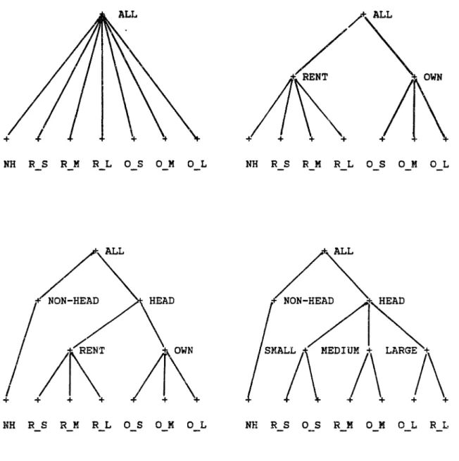
For the application at hand, let us introduce three steps of clustering. F~,~st, we bundle housing alternatives by size and

quality, then these clusters by tenure and type of building, and finally all headship alternatives versus the nonheadship alternative, see Figure 2-2 for a simple example. We can look at NMNL models in two ways: they represent hierarchically grouped clusters of alternatives with a larqe within group substitutability,

ana

we can

ALL

FIGURE 2-2: CLUSTERS OF SIMILAR ALTERNATIVES

~---~--~-~~--~--~~~--~-~---~--~--~--~---~ ~-~~-~---~-~--~--~~--~-~~-~---~--~~---~~---~ ALL ALL NH: non-head R: rented 0:

owned

s:

small

M:

medium

L:

large

- 30

-where each nucleus decides whether to head a household or not~ the heads decide about tenure, and owners and renters choose their Of course, this does not necessarily imply dwelling size and quality~

a temporal Oecomposition of the decision process. Figure 2-3 represents this second interpretation graphically, an~ the equivalence

to the representation of Figure 2-2 can be seen in each of the steps.

We can decompose the choice probabilities for a three-level hierarchical decision process into a marqinal choice probability at the highest level of the decision tree and conditional probabilities at each lower level (we suppress the index t for the individual household):

(2.5)

where

= probability of the headship choice Hi that is implied by choosing alternative i,

= probability of the tenure choice Ti implied

by choosing alternative i. given headship choice Hi' PS(SiIH;,Ti)

=

probability of the size choice Si implied by

alternative i, given headship choice Hi and

tenure choice Tie

At each level, the conditional choice probabi1ities have the

FIGURE 2-3: DECISION TREES FOR HOUSING ALTERNATIVES

~~----~~~---~~-~~---~----~~~--~-~--~-~--~---~

---~---~~~~~-~----~~~~~~-~~---~-~~---~~--~----NH R S R M R LOS 0 MOL NH R S R M R LOS 0 MOL

:f: ALL

LA~HEAD

NH R S R M R LOS 0 K 0 L NH R S 0 S R MOM 0 L R L NH: non-head R: rented 0: owned S: small M: medium L: large

- 32

-PS(Sd H1,T 1)

=

exp(

V(S1) )

ILexp(

V(Sj) ),

(summation over all size choices Sj possible in tenure choice Ti )

PT(T1

IH

1 )

=

exp(

u(T1 ) )

I

Lexp (

U(Tj) ),

(summation over all tenure choices Tj in headship choice Hi)

PH(Hl)

=

exp(

W(H1) )

I

Lexp (

W(Hj) ),

(summation over

all headship choices Hj )

In these choice probabilities, V(S1) denotes the utility, a consumer derives from dwelling size S;, and u(T;) ( w(H;) ) the utility from tenure choice Ti (headship choice Hi' respectively) implied by choosing alternative i .

At the higher levels, we assume that there is no utility per se of either headship or tenure over and above the utility derived from the alternatives underlying each tenure or headship choice. If

we

aggregate the utility provided by all alternatives Sj in tenure

category T; we obtain (McFadden, 1978):

(2.6) U(Ti) = log

~

exp ( Cj

*

v(Sj) )

jE

1i

and similarely for the aggregated utility of the headship choice Hi:

(2.7) w(H1 ) = log ~ exp ( dj ~ U(Tj ) )

Note that the attributes of the lowest level utility, e. g., income

and prices in the size choice, enter recursively, bottom-to-top, the utility of the tenure and heaOship choices. On the other hand,

decisions are clustere~ in a sequential fashion, top-to-bottom, as

Figures 2-2 and 2-3 suggest. Altogether we have achieved a simultaneous choice of hea~sh1p, tenure, an~ ~wel1ing size where prices as well as income are allowed to influence not only the size

and tenure choice, but also the headship decision and thus household formation.

The taste weights Cj and dj have to be estimated. The aggregate utility levels U(Ti) and w(Hi ) are called inclusive values of their

respective lower level alternatives because they can be interpreted as the surplus generated by these alternatives. The taste weights Cj and

dj are called dissimilarity parameters because they can be interpreted

as a measure of the substitutability among the respective lower level alternatives. For Cj and dj equal to one, the decision tree model

collapses to a simple multinomial logit choice model among all

alternatives~ If they are smaller than one, alternatives in the respective clusters are close

alternatives.

SUbstitutes relative to other

We can test whether the difference between the simple MNL model and the nested MNL model is significant. Usually, the MNL model has to estimated in a first stage to obtain initial values for the NMNL estimation. Thus, we have all ingredients of a lekilihood ratio test, see Table 5-13 for examples. Furthermore, we can construct a Wald

- 34 -MNL Simple the at test

appropriate formula. The of this test trinity is These test are tests of the

Finally,

asymptotic and small sample properties examined by Hausman and McFadden (1981). reported in the estimation results. Lagranqe multiplier test and evaluate this

estimates, see McFadden (1983) for the

test based on the estimateO dissimilarity coefficients in the NMNL model with their joint covariance matrix. For simple one-dimensional

tests we can look at the asymptotic t-statist1cs aroun~ one as

we can calculate a

Simple MNL functional specification versus the nested MNL model.

Thus, they amount to tests of the independence of irrelevant

alternatives property.

The random utility maximization interpretation 01 the NMNL

functional form rested on the integral formula (2.3). However, the

cumulative distribution function F is parameterized by the taste weights ail' bkr the dissimilarity coefficients Ci, dir and depends on

the data as well. If all similarity parameters are in the unit-interval, the underlying joint distribution of the disturbances

is well behaved and consistent with the microeconomic theory outlined

at the beginning of this section, independent of the explanatory

variables. With similarity parameters outside the unit-interval, this

consistency will hold only for a certain range of explanatory

variables, and it must be checked, whether this range includes the given data. ThiS check and a reconciliation of such NMNL models with the

random

utility maximization hypothesis is discussed in the followinge

2.2.3 The Relation Between Dissimilarity Parameters

and

the Random Utility Hypothesis

Let CT denote the similarity coefficient corresponding to the

first-order clusters of elementary alternatives (say, tenure categories), and dH the similarity coefficient corresponding to the

secon~-order clusters consisting of first-order clusters (saYr headship categories). The NMNL functional form specified in (2.5) is then equivalent to the following joint cumulative distribution function of the errors e i t in (2.1) (McFadden 1978):

(2.8) F{e1,···,eM) = exp { -G [ exp(-e1),···,exp(-eM) ] } with

L

L

L

l/CT CT!dH dH

(2.9) _{G[yl ' • • • 'YM]} =

Ys

) ) H T.H Se-T

where we sum over the highest-order clusters H, the first-order clusters T contained in each cluster H, and finally over the elemental alternatives S in each cluster T.

Two theorems provide the link between NMNL-models and the random utility maximization hypothesis (RUM). They are global statements in the sense of being independent of the realization of the explanatory

- 36

-Theorem 1 (Global Sufficiency) (McFadden 1979): Let 0 < dH S 1 and 0 < cT/~H S 1 for all T and H.

Th~n the HMNL model 1s consistent with RUM for any data.

Theorem 2 (Global Necessity) (Williams 1977, Daly anO Zachary 1979): Let dH > 1 or CT/dH > 1 for at least one T or H.

Then i t is always possible to construct data at which the NKNL model is inconsistent With RUM.

The question arises, whether this pO~Sibility of RUM-inconsistent data points is relevant for the data at hand. Theorem 2 leaves the possibility open that for the data given by the application, the NMNL model is consistent with RUM, and that the data points where the inconsistency occurs are insensible for the given application. Thus, the purpose of the remainder of this Section is to construct a discrete choice model that (1) is compatible with RUM, (2) has the same cumulative distribution function F for the given data points, and (3) preserves the choice probabilities of the original NMNL model. We shall give a necessary ana sufficient condition under which such a

construction is possible.

The failure of the random utility hypothesis occurs because the estimated dissimilarity coefficients prevent F from (2.8) being a

Lemma 1:

Let cT an~ dH > O.

(1) Then F 1s differentiable to

any

or~er, in particular, all mixed

partial

derivatives

eXisto

(2) F -> 1 for 81 ->00 , F -> 0 for 81 -> -~ (3) The choice probabilities derived from F obey

Pitt) = 1.

The Lemma follows from the obvious properties of (2.5),(2.8), and (2.9)e Thus, Theorem 2 implies the eXistence of at least one pOint in

which F has a negative mixed partial derivativer i . e. , a point of

negative marginal or joint "density".

We shall illustrate the effect of QH > 1 in the simplest case of a three-alternative, two-level NMNL-model in which the first two alternatives constitute a cluster.

distribution function

This model has the cumulative

F(e)

=

exp { - [ exp(-e1/d) + exp(-e2/d ) ]d - exp(ea) }.

Because of translation invariance (see Footnote 3), we can reduce F to the two dimensional space of differences without loosing information. Let v

=

e2~e1 and W

=

e3-e1- Their joint distribution function is

( l+exp(-v/d) )d-1

F*(v,w)

=

---( ~+exp(-v/d) )d + exp(-w)

with density

( l+exp(-v/d) )d-2

f*(V,w) = ---

*

exp(-w)

*

exp(-v/d)

*

discr,

- 38

-where the discriminant

term

2( l+eXp(-v/d) )d

d1scr

=

---0-1 ( l+eXp(-v/d) )d + exp(w) 0 signs the density f·.

For d < 1, discr > O.

However,

for ~ > 1,

f*(V,w) > 0 <=> W> log(d-l)-log(d+l) - ~ log(l+exp(-v/d».

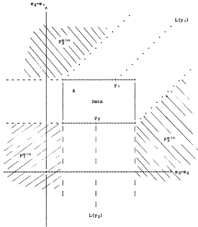
ThiS function approaches the constant log (d-l)-log(d+l) for v -> CO and a by this constant shifted 45-degree line for v -> -00. Thus, we can partition the (v,w)-plane in a part with nonnegative and a part with negative density, see Figure 2-4. Note that the latter part cannot be contained in any choice probability defining orthant.

If any of our data points is in the (shaded) area f* < 0, we will not be able to explain the data by preference maximization using the integral formula (2.3) underlying RUM. Moreover, if f*(e) < 0 for

some e, then the continuity of f* implies the eXistence of a point e This point need not necessarily be in the set {f* < oJ. Again, we cannot rationalize the data by RUM. Thus,

Theorem 3 (Local Necessity):

Let A be a set containing all data points.

Let anyone of the following conditions be true:

(1) A mixed partial derivative of F up to order M is negative

at a point in A.

(2) F exceeds unity at a point in A.

Then the construction of a RUM-compatible discrete choice model in A

~he proof is trivial: F cannot be a c.d.f. if it exceeds unity or

any of its associated marginal or the joint ~ensities is negative.

If neither of the conditions of Theorem 3 1s raised, we can indeed reconcile a NMNL-model with large dissimilarity coefficients

with random utility maximization:

Theorem 4 (Local Sufficiency):

Let A be an open interval containing all data points. Let both of the following conditions be true:

(1) All mixed partial derivative of F up to order Mare

nonnegative in A.

(2) F does not exceed unity at a point in A.

Then for any positive cT' dH eXists a continuation Fe of F, such that

(a) Fe is a cumulative distribution function,

(b) Fe generates the ~ame choice probabilities as F.

We will give the proof by construction. Figure 2-5 i.llustrates the

construction in the case of three alternatives, already underlying Figure 2-4. We first use the translation invariance principle to

reduce the dimension of the problem to )1-1: for any point y in RMw

let y* be the N=M-l dimensional vector (Y1-Y21 ••• 'Y1-YM)'· Correspondingly, we introduce A*, F*, and f* as the M-l dimensional counterparts of A, F, and f. For a set C, we use int(C), bnd(C), ext(C), and clo(C) to denote the interior, the boundary, the exterior,

40

-FIGURE 2-4: THREE ALTERNATIVES: CHOICE PROBABILITIES AND DENSITY

===========~========================================== ==========

e2+Y2 > e 1+Y1

e2+Y2 > e3+Y3

<=> e2-e1 > Y1-Y2

(e2-e 1)-(e3-e 1) > (Y1-Y3)-(Y1-Y2)

III< + y <=> e3+Y3 > e 1+Y1 e3+Y3 > e2+Y2

or

e1+Y1 > e2+Y2 e1+Y1 > e3+Y3 e1-e2 > Y1-Y2 e1-e 3 > Y1-Y3

I

I

I

e3-e1 > Y1-Y3

I

(e3- e 1)-(e2-e 1) > (Y1-Y2)-(Y1-Y3)

I

I

---+--->

e3-e 2

I

d-l f*(V,w) > 0 + - - - -~-_- --~-:--- log d+l

FIGURE 2-5: CHOICE PROBABILITY PRF~ERVING CHOICE MODELS ===============================~==~~===================

- - +---+---+

A

42

-and the closure of C, respectively.

For each

y.,

we can partit.ion RN according to the M choice probability defining open sets

and the M separating half-hyperplanes

The sets Pi(Y~) and Li{Y*) will be important at the boundary of A,

an~ it is convenient to define for y* in bnd(A*):

Pmin

_

;

-y* in A·

and

L(Y*) = L;(Y*) with i such that L;(Y*)

n

clo(A*) is empty.

The p~in define the smallest choice probability of alternative i attainable in clO(A-) where this well-defined minimum occurs for each i at one of M corners of the interval A*. The L(Y*) define the

half-hyperplane pointing outward of A*. This is well-defined except

for the above mentioned M corners. Here, we define:

We now

construct

a choice model

which

has identical choice

probabilities in A* by shifting all probability mass outside of A*

onto the boundary of A* in a

way

which does not distort the oriqinal

We define

f*C(y) = f ·(y) for y in A

It:,

f*C(y)

₌

_fdF* for y in bnd(A*),

L{Y*)

f *C(y) _{= 0 for} Y in ext(A*). We have to show:

(i) f*c _nonnegativeu

(ii) f*c _{integrates to}

_one,

(iii) Pt(i) =

f

_{dF =}

f

_dFc_•

P_t(i) P_t (i) To (i) :

We only need to show the nonnegativity at the boundary. Case 1: y is at one of the M corners defining p~in.

Then the f*C(y) is a choice probability which is always nonnegative for positive cT, dH by Lemma 1.

lim

.f

_dF· Pj (Y*-hZj ) Case 2: y otherwise. Then

f

dF"

=

L ; (y.) l/h (

r

dF* -h -> 0 ~ Pj (y*)

where j is an arbitrary index other than i and z a vector of zeroes

except a one at the j-th component. ThiS; however, defines the j-th'

marginal density of F* which is nonnegative due to assumption (1). To (ii):

Decompose

f

f*C(U)dU =

f

f*C(U)dU +

RN A*

f

f*C(U)dU + ext(A*)

f

f·C(u)du bna{Aqt) =

.f

ciF* +

f

dF* ₊

_a

=

_fdF*

=

1, A* RN\A* _RN

44 -To (iii): +

f

dF* Pi(y*)n(RN\A*)

.- f

dF*~

+ Pi (Y*)()A*

=

f

dF-C Pi(y *>nbnd (A *)

f

dF -c +

f

dF

~

C

=

P1(Y *)()A* Pi (y*)n(RN\A*) This proves Theorem 4.

f

dF$C

Theorem 4 extends the usefulness of NMNL-models by reconciling large dissimilarity coefficients with random utility maximization, providedq conditions (1) and (2) hold. In practice, these conditions can be checked by evaluating the density and cumulative distribution function at the corners of an interval containing the data.

Furthermore, the idea behind Theorem 4 can be exploited to construct a large class of RUM-compatible discrete choice models. Any function which is translation invariant in the sense of Footnote 3 and obeys conditions (1) and (2) of the Theorem in an interval containing the data can be extended to a cumulative distribution function

2.3 Estimation Techniques

2.3.1 Econometric Theory and Numerical Analysis

The likelihood function of the hierarchical choice model are the logarithms of the choice probabilities (205), cumulated over all

consumers. Thus, we can estimate the model by maximizing over the taste weights a i l ' b_{k •} an~ the similarity coefficientR C;I die Because the full information maximum likelihood function is highly nonlinear in the similarity parameters, this approach is costly. As an alternative, we can exploit the recursive structure in (2.5) and estimate sequentially by level of clusterinq. This approach has been

applied to a large number of problems in transportation, energy

demand, and urban economics, see Domencich and McFadden (1975) or Anas However, the sequential estimator is inefficient, especially for complex decision trees. Furthermore, i t can not embody parameter restrictions across branChes/clusters of alternatives.

The first point relates to the flow of information: the sequential estimator uses all the information of the lower branches to

estimate the dissimilarity coefficients at the upper levels, but not

cunverselyv Amemiya (1978) noted that the standard errors of the

estimated coefficients at the upper levels have to be corrected for the presence of lower level estimated coefficients, McFadden (1981) provides the proper formulae. Evaluating these corrections is expensive

and

greatly reduces the computational advantaqes

over

the FIKL estimator, see Small and Brownstone (1982). The second point is more important: if the alternatives in different branches have taste

46

-weights in common, a proportionality constraint has to be fUlfilled

which is non-trivial for the case of at least two elementary alternatives in at least two branches:

(h/c) 1

The sequential estimator estimates (b!C) 1 and (b/C) 2 in the first

stage choices, then C1 and c2 in the choice between the branches. A

common b implies

Howeverr imposing this restriction Oestroys the sequential

decomposition and leads us back to fUll information maximum

likeli.hood. The proportionality constraints could be imposed by an

iterative procedure where the Ci from the sequential estimation as described are used in a seconO sequential estimate to scale the (b/C); as (b/Ci);' calculate new Ci, and so on. This iteration will further reduce the computational advantages over FIML estimation in addition to the necessary correction of the standard errors, in particular so

in higher level trees.

We therefore prefer joint estimation and use the modified

quadratic hill-climbing method developed by Goldfeld and Quandt (1972) with analytical first and numerical second derivatives. This procedure proved computationally fairly efficient compared with BHHH

(1982) report similar experiences with BHHH as compare~ to a method of scoring. The reason for the relative poor performance of the BHHH alqorithm seems to be the highly nonlinear dependence of the likelihood function on the dissimilarity parameters. In particular, the function and its gradient have a singularity in ci or di at zero. The singularity is well behaved for the likelihood, but is a pole for the gradient. Thus, the outer product of the gradients is ill-behaved and a ba~ approximation of the hessian for small values of the dissimilarity parameters.

This unpleasant behavior of the l~kelihood function requires a careful numerical analysis of the algorithms involved. In particular, the data should be normalized to prevent the multiplication of very

small with very

large

numbers and

numerical extinction. The appendix lists a FORTRAN program for the full information maximum likelihood estimation of NKNL models which emboOies all these considerations.

48

-2.3.2 Elasticities and Goodness-of-Fit Measures

Following the random utility maximization theory and equation (2.2), the estimated parameters represent the taste weights of the respective explanatory variables in the deterministic part of the indirect utility function Vit. For a more intuitive interpretation of their magnitudes, the taste weights can be transformed into elasticities of the choice probabilities With respect to the various explanatory variables: ?logp(i) (2.10).---

=

ak * Xjk * ( -p(j) + ks * lie ')109 Xj k + kT * (1!C-l/d) * Q(S) + kH * (d-l)/d * Q(S) * Q(T) )

where ks = 0 if i and j are in the same size category

= 1 otherwise

kT = 0 if i and j are in the same tenure category

=

1 otherwise

kH = 0 if i and j are in the same headship category

= 1 otherwise

c,d

₌

similarity parameters: c=cr and d=dH

Q(S)

=

conditional choice probability ps(SjIHj,Tj )

Q(T)

--

condit1.onal choice probability PT(TjIHJ)

These elasticities measure the percentage Change of the probability to choose alternative i, when the k-th attribute of alternative j is changed by one percent. Note that for the cross elasticities the difference between i and j enters only through the "switches" kSI kT'

and kH. The structure of the tree is therefore directly reflected in

and d are in the unit interval, equation (2.10) implies descending elasticities with the "distance" in the tree, i. e., elasticities are larger within than between branches. This plausible structure is

destroyed fo~ dissimilarity parameters larger than one, hinting to alternative tree specificationso

Derived from a highly non-linear model, elasticities at variable means are generally different from mean individual elasticities, and in interpreting the e1asticities, one should keep the absolute level of the choice-probabilities in mind; the elasticities tend to be very high at very low probabilities and vice versa, ref~ectin9 saturation effects.

Three scalar measures of performance or fit will be used in the applications- of Chapters 3 and S. Arnemiya (1981) provides an extensive review. The straightforward discrete analogy to the continuous R2 uses the sum of squared errors:

(2.1.1.)

where

L L

(yit-Pi·db»2 / Pi t(b) 1 - ---

LL

(yi t -Pi t(0»2 / Pu(b) , -to

Pit ~enotes the predicted choice prObabilities of alternative i for consumer t, evaluated at the optimal parameter values b or at zero, and Y;t the actual response6 • However, this measure has little discriminatory power for well specified models. A more satisfactory measure can be constructed from the ratio of the likelihood at the

estimated parameters and the likelihood with taste weights at zero and similarity parameters at one. One minus this ratio behaves like the

~ 50

-continuous R2 , see Mcfadden (1973):

(2.12)

L{b) 1 -

---L(O)

Domencich and McFadden (1975) give a comparison between these two measures of fit and their discriminatory power. As a third measure of fit, we compare actual with predicted individual choices which is a fairly stringent, thouqh erratic criteriono Note that discrete choice

mo~els produce two predictions of the aggregate choice probabilities:

(2.13) f(i)

=+~Pt(i)

t

(2.14) f(i)

=

n(i)/T

with n(i) = number { t

I

Pt(i) = max Pt(j) } j=l •• M T

=

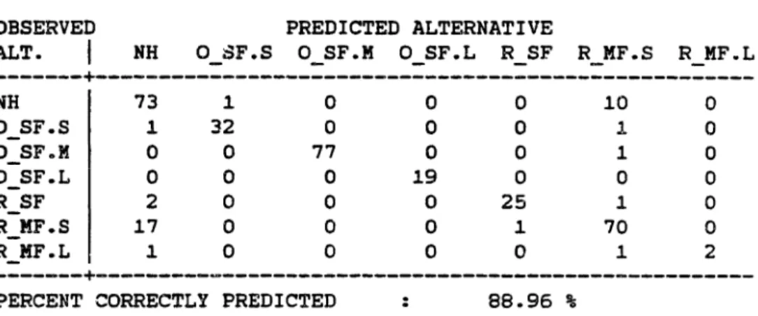
sample size

The erratic nature of the percentage of correct predictions is due the integer constraint in (2.14). We can disaggregate this measure into the form of a success table in which observed and predicted alternatives are crosstabulated and the off-diagonal elements show the mispredictions.

2.3.3 Aggregate Probability Shares

The aggregate probability shares f(i), i=l •• M, where M denotes the number of alternatives, from equation (2.14) can be used for prediction and poliCY analysis. They should reproduce the aggregate shares in the population q(i) as close as possible. A multinomial speCification with a fUll set of alternative speCific constants will

always reproduce the sample shares exactly which can be seen by adding up the first order conditions of the MNL-like11hood function with respect to the alternative specific dummies. This property is not carried over to the nested model. Anas (1982) gives some numerical

examples for this bias. However, a fUll set of alternative specific constants still saturates the model and we can always solve the

non1inear system of M-l equations in these constants to adjust the

aggregated shares. This suggests the following two stage procedure:

first we estimate all parameters freely; then, we solve this

likelihood This will the slope nonlinear equation system evaluated at the slope parameters of the first stage. The second step can be achieved by minimizing the sum of squareO deviations of fitted to actual aggregated shares. This two

stage procedure is consistent, but does not provide efficient

parameter estimates. Usually, the adjustment necessary is very small, and so the loss in efficiency.

A more satisfactory approach is to maximize the function subject to the B-1 constraints f(i)=q(i), i=2 •• M. yield efficient estimates (Coslett, 1981) where also

- 52

-Unfortunately, the nonlinear equation system can not be solved analytically, making a costly constraint maximization necessary which involves additional M-l nuisance parameters and in general the solution of a saddlepoint problem as opposed to a simple maximization problem. Furthermore, the application of KUhn-Tucker type algorithms is not possible because the constraints f(i)=q(i) are highly nonlinear in the alternative specific constants. We will only use the two stage procedure. We apply this procedure in Chapter Five to adjust our baseline estimates before making predictions and policy simulations.

2.3.4 Choice Based Sampling

The problem of fitting the known aggregate sample shares is related to the problems generated by choice based sampling. Choice based samples may arise in two ways: the data may originally be

collected by sampling according to the observed choice. This is the case when we interview a fixed number of homeowners and a fixed number of renters and these numbers do not reflect the proportions in the population. Second, we may start from a large random sample. Typically, however, some choices have very low, others very high market shar~s. To achieve precise estimates for all choices, the overall sample size of a smaller random subsample drawn for estimation has to be large enough that even the smallest cell has a sufficient

number of observations. This will yield very large cell counts for the popular choices. We can substantially decrease estimation costs by oversampling the infrequent choices, undersampling the frequent choices, and then treating our subsample as a choice based sample. We will make heavy use of this technique in Chapter Five.

Given a choice based sample, the parameters have to be estimated to predict the population, not the sample shares. Without a correction, the estimates are inconsistent (HeCkma~1979). Thus the efficient full information maximum likelihood estimator is again the Coslett (1981) estimator mentioned in the previous subsection and involves the solution of a saddlepoint problem with H-l additional nuisance parameters. Alternative estimators are discussed in Manski and McFadden (1981) of which we mention the two most important.

- 54

-First, we can compensate for choice based sampling by weighting the observations inversely to the ratio of over or undersampling. This estimator (weighted exogenous sampling maximum likelihood, WESI1L, Manski and Lerma~1977) is as cheap to compute as the normal maximum likelihood estimator. Second, we can maximize the likelihood of an endogenously sampled observation conditional on its exogenous characteristics. This estimator (conditional maximum likelihood, CML, Hsieh, Manski, and McFadde~1983) has a slightly more complicated likelihood function compared to the WESML estimator. Both estimators yield consistent estimates without the introduction of additional nuisance parameters, but there are not efficient compared to the Coslett estimator. However, the efficiency loss seems to be very small as indicated in McFadden, HSieh, and Manski (1983) or McFadden, Winston, and Boersch-Supan (1984).

Therefore, and for its simplicity, we will only use the WESML estimator. The resulting likelihood functioll in our case is

(2.15) L =

where i t denotes the chosen alternative of household t q(i) the proportion of alternative i in population f(i) the proportion of alternative i in the sample p(i,b) the choice probability according to (205) b vector of parameters

The covariance matrix of the estimated b can be derived by an

(2.16)

AT HT

where b* lies on a line segment between b and b~.

Under the appropriate regularity conditions (Manski and McFadden 1981), we can apply a uniform law of large numbers (Jennrich 1969) to

show

(2.17) _HT ~~> _{H = E( --- ) ,}

and a uniform central limit theorem (Jennrich 1969) to yield

db'

v

= E( --- --- )0 (2.18) where (2.19) Thus, AT

~~>

N ( 0 , V ) dW(t) log P(blt) dW(t) log P(b*) (2.20) ~ ( b - b*) --> N ( 0 , H-1 _{V H-1 ).} As a consequence, (2.21) f(i)

f

q(i) => H

f

V,

because H includes the weights linearly, but V quadratically. Thus, the inverse hessian does no longer provide an estimate for the covariance matrix of the estimated b. In the estimation, we will use the sample hessian to approximate H and the sample outer product of the gradient to approximate V, both evaluated at the optimum.

Tne likelihood function (2.15) is a special case of the WESML estimator insofar, as we assume independent draws of households t, each with one choice of its housing alternative. This deviates from

- 56

-counts m(i,t) are observed. In our case, m(i,t)=l for i=it.the chosen alternative,

a

otherwise. In the case of mUlti.ple cell counts, which are distributed multinomially, the negative covariance between m(i,t) and m(j,s) may reduce the variance (2.19). Depending on the way the sample 1s drawn, either E( m{i,t) m(i,s) ) or E( m(i,t) m(j,t» will

2.4 Conclusions

This chapter provided the econometric tools for thiS thesiSe We will cast all housing alternatives in a finite set of alternatives, structure them in the form of a hierarchical decision tree, and calculate the nested multinomial loqit choice probabilities for each alternativee

These choice probabilities can be rationalized by utility

maximization behavior of the consumers, but only under certain parameter restrictions. We developed necessary and sufficient

conditions for the consistency of random utility maximization with the nested multinomial logit specification in the case of dissimilarity

parameters in and outside the unit interval. If we maintain utility

maximization as underlying structural behavior, we can interpret the

v~olat1on of these conditions (the case of Theorem 3) as a hint to misspec1ficat1on of either the in~irect utility function (2.2) or,

more important, the tree structure. Alternative tree structures may be derived from the elasticity patterns created by (2.10)~

Because of the inefficiency of sequential estimation procedures

and their inability to embody equal utility weights for prices and

income across tenure and headship clusters, we use full information maximum likelihood estimation throughout the thesis. This has become

- 58

-2.5 Footnotes to Chapter 2

(1) The requirement to be finite-valued implies that ties in the pairwise comparison of utilities occur only with probability zero.

(2) We impose linearity and additive separability of the indirect utility function in the definition of RUM. In the language of McFadden (1981), such models are defined as AIRUM-compatible.

(3) Note that the definition of the indirect utility function implies translation invariance of the choice probabilities in the following

sense:

Pu(i)

=

Pu+c(i) for all constants c and all utility vectors U in RM, or,

G(y+c) = G(y) + c for all constants c and all vectors y in RM+,

where G denotes the generating function (2.9).

(4) This amounts to including M-l alternative specific constants D; interacting with the

yi

and using a common parameters bl for all alternatives which can be seen by the transformation

Y

i·

D ;~b1 = Y~.a;1 •

(5) The random utility maximization hypothesis as stated in Section 2.2 is only one rationalization of observed choice behavior with the notion of a homo economicus. Failure of RUM does not necessarily preclude the possibility that such a model is rational in an axiomatic sense, i . e., that i t fUlfills the axiom of stochastically revealed preferencesD This is a combinatorial problem of a large dimension. See McFadden and Richter (1979).

(6) The sum of the squared residuals can be weighted in several ways~

The natural weights are the true choice probabilities. As the best available estimates, we replace them by their maximum likelihood estimates. See Amemiya (1981) for alternatives.

~

The Libraries

Massachusetts Institute of Technology Cambridge, Massachusetts 02139 Institute Archives and Special Collections

Room 14N·118 (617) 253-5688

There is no text material missing here. Pages have been incorrectly numbered.

63

-CHAPTER THREE

THE INFLUENCE OF HOUSEHOLD FORMATION ON HOUSING DEMAND

************** ******************** *****~***********.*~**** *~****.*******.************

********

******** ******* ******* ****** ****~** ******** ******** ***~*1t** ********* *********

*-******

*******JIr ******** ****** *******

*******

******

******** ******* ********aa***************k* *****************e****** ******************** ~*****.******* \