EUROPEAN ORGANIZATION FOR NUCLEAR RESEARCH (CERN)
CERN-PH-EP-2013-143 LHCb-PAPER-2013-036 11th October 2013
Observation of B
s
0
-B
0
s
mixing and
measurement of mixing frequencies
using semileptonic B decays
The LHCb collaboration†
Abstract
The Bs0 and B0 mixing frequencies, ∆ms and ∆md, are measured using a data
sample corresponding to an integrated luminosity of 1.0 fb−1 collected by the LHCb experiment in pp collisions at a centre of mass energy of 7 TeV during 2011. Around 1.8×10⁶ candidate events are selected of the type B(s)0 → D−(s)µ+(+ anything), where about half are from peaking and combinatorial backgrounds. To determine the B decay times, a correction is required for the momentum carried by missing particles, which is performed using a simulation-based statistical method. Associated production of muons or mesons allows us to tag the initial-state flavour and so to resolve oscillations due to mixing. We obtain
∆ms= (17.93 ± 0.22 (stat) ± 0.15 (syst)) ps−1,
∆md= (0.503 ± 0.011 (stat) ± 0.013 (syst)) ps−1.
The hypothesis of no oscillations is rejected by the equivalent of 5.8 standard deviations for Bs0 and 13.0 standard deviations for B0. This is the first observation of Bs0 mixing to be made using only semileptonic decays.
To be published in Eur. Phys. J. C
c
CERN on behalf of the LHCb collaboration, license CC-BY-3.0.
†Authors are listed on the following pages.
LHCb collaboration
R. Aaij40, B. Adeva36, M. Adinolfi45, C. Adrover6, A. Affolder51, Z. Ajaltouni5, J. Albrecht9, F. Alessio37, M. Alexander50, S. Ali40, G. Alkhazov29, P. Alvarez Cartelle36, A.A. Alves Jr24,37, S. Amato2, S. Amerio21, Y. Amhis7, L. Anderlini17,f, J. Anderson39, R. Andreassen56,
J.E. Andrews57, F. Andrianala37, R.B. Appleby53, O. Aquines Gutierrez10, F. Archilli18,
A. Artamonov34, M. Artuso58, E. Aslanides6, G. Auriemma24,m, M. Baalouch5, S. Bachmann11, J.J. Back47, C. Baesso59, V. Balagura30, W. Baldini16, R.J. Barlow53, C. Barschel37, S. Barsuk7, W. Barter46, Th. Bauer40, A. Bay38, J. Beddow50, F. Bedeschi22, I. Bediaga1, S. Belogurov30,
K. Belous34, I. Belyaev30, E. Ben-Haim8, G. Bencivenni18, S. Benson49, J. Benton45, A. Berezhnoy31, R. Bernet39, M.-O. Bettler46, M. van Beuzekom40, A. Bien11, S. Bifani44, T. Bird53, A. Bizzeti17,h, P.M. Bjørnstad53, T. Blake37, F. Blanc38, J. Blouw11, S. Blusk58,
V. Bocci24, A. Bondar33, N. Bondar29, W. Bonivento15, S. Borghi53, A. Borgia58,
T.J.V. Bowcock51, E. Bowen39, C. Bozzi16, T. Brambach9, J. van den Brand41, J. Bressieux38, D. Brett53, M. Britsch10, T. Britton58, N.H. Brook45, H. Brown51, I. Burducea28, A. Bursche39,
G. Busetto21,q, J. Buytaert37, S. Cadeddu15, O. Callot7, M. Calvi20,j, M. Calvo Gomez35,n, A. Camboni35, P. Campana18,37, D. Campora Perez37, A. Carbone14,c, G. Carboni23,k, R. Cardinale19,i, A. Cardini15, H. Carranza-Mejia49, L. Carson52, K. Carvalho Akiba2, G. Casse51, L. Castillo Garcia37, M. Cattaneo37, Ch. Cauet9, R. Cenci57, M. Charles54, Ph. Charpentier37, P. Chen3,38, N. Chiapolini39, M. Chrzaszcz25, K. Ciba37, X. Cid Vidal37, G. Ciezarek52, P.E.L. Clarke49, M. Clemencic37, H.V. Cliff46, J. Closier37, C. Coca28, V. Coco40, J. Cogan6, E. Cogneras5, P. Collins37, A. Comerma-Montells35, A. Contu15,37, A. Cook45, M. Coombes45, S. Coquereau8, G. Corti37, B. Couturier37, G.A. Cowan49, D.C. Craik47, S. Cunliffe52, R. Currie49, C. D’Ambrosio37, P. David8, P.N.Y. David40, A. Davis56, I. De Bonis4, K. De Bruyn40, S. De Capua53, M. De Cian11, J.M. De Miranda1, L. De Paula2, W. De Silva56, P. De Simone18, D. Decamp4, M. Deckenhoff9, L. Del Buono8, N. D´el´eage4, D. Derkach54, O. Deschamps5, F. Dettori41, A. Di Canto11, H. Dijkstra37, M. Dogaru28, S. Donleavy51, F. Dordei11, A. Dosil Su´arez36, D. Dossett47, A. Dovbnya42, F. Dupertuis38, P. Durante37, R. Dzhelyadin34, A. Dziurda25, A. Dzyuba29, S. Easo48, U. Egede52, V. Egorychev30,
S. Eidelman33, D. van Eijk40, S. Eisenhardt49, U. Eitschberger9, R. Ekelhof9, L. Eklund50,37, I. El Rifai5, Ch. Elsasser39, A. Falabella14,e, C. F¨arber11, G. Fardell49, C. Farinelli40, S. Farry51, D. Ferguson49, V. Fernandez Albor36, F. Ferreira Rodrigues1, M. Ferro-Luzzi37, S. Filippov32, M. Fiore16, C. Fitzpatrick37, M. Fontana10, F. Fontanelli19,i, R. Forty37, O. Francisco2, M. Frank37, C. Frei37, M. Frosini17,f, S. Furcas20, E. Furfaro23,k, A. Gallas Torreira36,
D. Galli14,c, M. Gandelman2, P. Gandini58, Y. Gao3, J. Garofoli58, P. Garosi53, J. Garra Tico46, L. Garrido35, C. Gaspar37, R. Gauld54, E. Gersabeck11, M. Gersabeck53, T. Gershon47,37, Ph. Ghez4, V. Gibson46, L. Giubega28, V.V. Gligorov37, C. G¨obel59, D. Golubkov30, A. Golutvin52,30,37, A. Gomes2, P. Gorbounov30,37, H. Gordon37, C. Gotti20,
M. Grabalosa G´andara5, R. Graciani Diaz35, L.A. Granado Cardoso37, E. Graug´es35,
G. Graziani17, A. Grecu28, E. Greening54, S. Gregson46, P. Griffith44, O. Gr¨unberg60, B. Gui58, E. Gushchin32, Yu. Guz34,37, T. Gys37, C. Hadjivasiliou58, G. Haefeli38, C. Haen37,
S.C. Haines46, S. Hall52, B. Hamilton57, T. Hampson45, S. Hansmann-Menzemer11, N. Harnew54, S.T. Harnew45, J. Harrison53, T. Hartmann60, J. He37, T. Head37, V. Heijne40, K. Hennessy51,
P. Henrard5, J.A. Hernando Morata36, E. van Herwijnen37, M. Hess60, A. Hicheur1, E. Hicks51, D. Hill54, M. Hoballah5, C. Hombach53, P. Hopchev4, W. Hulsbergen40, P. Hunt54, T. Huse51, N. Hussain54, D. Hutchcroft51, D. Hynds50, V. Iakovenko43, M. Idzik26, P. Ilten12,
R. Jacobsson37, A. Jaeger11, E. Jans40, P. Jaton38, A. Jawahery57, F. Jing3, M. John54, D. Johnson54, C.R. Jones46, C. Joram37, B. Jost37, M. Kaballo9, S. Kandybei42, W. Kanso6, M. Karacson37, T.M. Karbach37, I.R. Kenyon44, T. Ketel41, A. Keune38, B. Khanji20,
O. Kochebina7, I. Komarov38, R.F. Koopman41, P. Koppenburg40, M. Korolev31, A. Kozlinskiy40, L. Kravchuk32, K. Kreplin11, M. Kreps47, G. Krocker11, P. Krokovny33, F. Kruse9, M. Kucharczyk20,25,j, V. Kudryavtsev33, K. Kurek27, T. Kvaratskheliya30,37,
V.N. La Thi38, D. Lacarrere37, G. Lafferty53, A. Lai15, D. Lambert49, R.W. Lambert41, E. Lanciotti37, G. Lanfranchi18, C. Langenbruch37, T. Latham47, C. Lazzeroni44, R. Le Gac6, J. van Leerdam40, J.-P. Lees4, R. Lef`evre5, A. Leflat31, J. Lefran¸cois7, S. Leo22, O. Leroy6, T. Lesiak25, B. Leverington11, Y. Li3, L. Li Gioi5, M. Liles51, R. Lindner37, C. Linn11, B. Liu3, G. Liu37, S. Lohn37, I. Longstaff50, J.H. Lopes2, N. Lopez-March38, H. Lu3, D. Lucchesi21,q, J. Luisier38, H. Luo49, F. Machefert7, I.V. Machikhiliyan4,30, F. Maciuc28, O. Maev29,37,
S. Malde54, G. Manca15,d, G. Mancinelli6, J. Maratas5, U. Marconi14, P. Marino22,s, R. M¨arki38, J. Marks11, G. Martellotti24, A. Martens8, A. Mart´ın S´anchez7, M. Martinelli40,
D. Martinez Santos41, D. Martins Tostes2, A. Martynov31, A. Massafferri1, R. Matev37, Z. Mathe37, C. Matteuzzi20, E. Maurice6, A. Mazurov16,32,37,e, J. McCarthy44, A. McNab53, R. McNulty12, B. McSkelly51, B. Meadows56,54, F. Meier9, M. Meissner11, M. Merk40,
D.A. Milanes8, M.-N. Minard4, J. Molina Rodriguez59, S. Monteil5, D. Moran53, P. Morawski25, A. Mord`a6, M.J. Morello22,s, R. Mountain58, I. Mous40, F. Muheim49, K. M¨uller39,
R. Muresan28, B. Muryn26, B. Muster38, P. Naik45, T. Nakada38, R. Nandakumar48, I. Nasteva1, M. Needham49, S. Neubert37, N. Neufeld37, A.D. Nguyen38, T.D. Nguyen38, C. Nguyen-Mau38,o, M. Nicol7, V. Niess5, R. Niet9, N. Nikitin31, T. Nikodem11, A. Nomerotski54, A. Novoselov34, A. Oblakowska-Mucha26, V. Obraztsov34, S. Oggero40, S. Ogilvy50, O. Okhrimenko43,
R. Oldeman15,d, M. Orlandea28, J.M. Otalora Goicochea2, P. Owen52, A. Oyanguren35, B.K. Pal58, A. Palano13,b, T. Palczewski27, M. Palutan18, J. Panman37, A. Papanestis48, M. Pappagallo50, C. Parkes53, C.J. Parkinson52, G. Passaleva17, G.D. Patel51, M. Patel52, G.N. Patrick48, C. Patrignani19,i, C. Pavel-Nicorescu28, A. Pazos Alvarez36, A. Pellegrino40, G. Penso24,l, M. Pepe Altarelli37, S. Perazzini14,c, E. Perez Trigo36, A. P´erez-Calero Yzquierdo35, P. Perret5, M. Perrin-Terrin6, L. Pescatore44, E. Pesen61, K. Petridis52, A. Petrolini19,i,
A. Phan58, E. Picatoste Olloqui35, B. Pietrzyk4, T. Pilaˇr47, D. Pinci24, S. Playfer49, M. Plo Casasus36, F. Polci8, G. Polok25, A. Poluektov47,33, E. Polycarpo2, A. Popov34,
D. Popov10, B. Popovici28, C. Potterat35, A. Powell54, J. Prisciandaro38, A. Pritchard51, C. Prouve7, V. Pugatch43, A. Puig Navarro38, G. Punzi22,r, W. Qian4, J.H. Rademacker45, B. Rakotomiaramanana38, M.S. Rangel2, I. Raniuk42, N. Rauschmayr37, G. Raven41,
S. Redford54, M.M. Reid47, A.C. dos Reis1, S. Ricciardi48, A. Richards52, K. Rinnert51, V. Rives Molina35, D.A. Roa Romero5, P. Robbe7, D.A. Roberts57, E. Rodrigues53, P. Rodriguez Perez36, S. Roiser37, V. Romanovsky34, A. Romero Vidal36, J. Rouvinet38,
T. Ruf37, F. Ruffini22, H. Ruiz35, P. Ruiz Valls35, G. Sabatino24,k, J.J. Saborido Silva36, N. Sagidova29, P. Sail50, B. Saitta15,d, V. Salustino Guimaraes2, B. Sanmartin Sedes36, M. Sannino19,i, R. Santacesaria24, C. Santamarina Rios36, E. Santovetti23,k, M. Sapunov6,
A. Sarti18,l, C. Satriano24,m, A. Satta23, M. Savrie16,e, D. Savrina30,31, P. Schaack52, M. Schiller41, H. Schindler37, M. Schlupp9, M. Schmelling10, B. Schmidt37, O. Schneider38, A. Schopper37, M.-H. Schune7, R. Schwemmer37, B. Sciascia18, A. Sciubba24, M. Seco36, A. Semennikov30, K. Senderowska26, I. Sepp52, N. Serra39, J. Serrano6, P. Seyfert11,
M. Shapkin34, I. Shapoval16,42, P. Shatalov30, Y. Shcheglov29, T. Shears51,37, L. Shekhtman33, O. Shevchenko42, V. Shevchenko30, A. Shires9, R. Silva Coutinho47, M. Sirendi46,
T. Skwarnicki58, N.A. Smith51, E. Smith54,48, J. Smith46, M. Smith53, M.D. Sokoloff56, F.J.P. Soler50, F. Soomro38, D. Souza45, B. Souza De Paula2, B. Spaan9, A. Sparkes49, P. Spradlin50, F. Stagni37, S. Stahl11, O. Steinkamp39, S. Stevenson54, S. Stoica28, S. Stone58,
B. Storaci39, M. Straticiuc28, U. Straumann39, V.K. Subbiah37, L. Sun56, S. Swientek9, V. Syropoulos41, M. Szczekowski27, P. Szczypka38,37, T. Szumlak26, S. T’Jampens4,
M. Teklishyn7, E. Teodorescu28, F. Teubert37, C. Thomas54, E. Thomas37, J. van Tilburg11,
V. Tisserand4, M. Tobin38, S. Tolk41, D. Tonelli37, S. Topp-Joergensen54, N. Torr54,
E. Tournefier4,52, S. Tourneur38, M.T. Tran38, M. Tresch39, A. Tsaregorodtsev6, P. Tsopelas40, N. Tuning40, M. Ubeda Garcia37, A. Ukleja27, D. Urner53, A. Ustyuzhanin52,p, U. Uwer11, V. Vagnoni14, G. Valenti14, A. Vallier7, M. Van Dijk45, R. Vazquez Gomez18,
P. Vazquez Regueiro36, C. V´azquez Sierra36, S. Vecchi16, J.J. Velthuis45, M. Veltri17,g,
G. Veneziano38, K. Vervink37, M. Vesterinen37, B. Viaud7, D. Vieira2, X. Vilasis-Cardona35,n, A. Vollhardt39, D. Volyanskyy10, D. Voong45, A. Vorobyev29, V. Vorobyev33, C. Voß60,
H. Voss10, R. Waldi60, C. Wallace47, R. Wallace12, S. Wandernoth11, J. Wang58, D.R. Ward46, N.K. Watson44, A.D. Webber53, D. Websdale52, M. Whitehead47, J. Wicht37, J. Wiechczynski25, D. Wiedner11, L. Wiggers40, G. Wilkinson54, M.P. Williams47,48, M. Williams55, F.F. Wilson48, J. Wimberley57, J. Wishahi9, W. Wislicki27, M. Witek25, S.A. Wotton46, S. Wright46, S. Wu3, K. Wyllie37, Y. Xie49,37, Z. Xing58, Z. Yang3, R. Young49, X. Yuan3, O. Yushchenko34,
M. Zangoli14, M. Zavertyaev10,a, F. Zhang3, L. Zhang58, W.C. Zhang12, Y. Zhang3, A. Zhelezov11, A. Zhokhov30, L. Zhong3, A. Zvyagin37.
1Centro Brasileiro de Pesquisas F´ısicas (CBPF), Rio de Janeiro, Brazil 2Universidade Federal do Rio de Janeiro (UFRJ), Rio de Janeiro, Brazil 3Center for High Energy Physics, Tsinghua University, Beijing, China 4LAPP, Universit´e de Savoie, CNRS/IN2P3, Annecy-Le-Vieux, France
5Clermont Universit´e, Universit´e Blaise Pascal, CNRS/IN2P3, LPC, Clermont-Ferrand, France 6CPPM, Aix-Marseille Universit´e, CNRS/IN2P3, Marseille, France
7LAL, Universit´e Paris-Sud, CNRS/IN2P3, Orsay, France
8LPNHE, Universit´e Pierre et Marie Curie, Universit´e Paris Diderot, CNRS/IN2P3, Paris, France 9Fakult¨at Physik, Technische Universit¨at Dortmund, Dortmund, Germany
10Max-Planck-Institut f¨ur Kernphysik (MPIK), Heidelberg, Germany
11Physikalisches Institut, Ruprecht-Karls-Universit¨at Heidelberg, Heidelberg, Germany 12School of Physics, University College Dublin, Dublin, Ireland
13Sezione INFN di Bari, Bari, Italy 14Sezione INFN di Bologna, Bologna, Italy 15Sezione INFN di Cagliari, Cagliari, Italy 16Sezione INFN di Ferrara, Ferrara, Italy 17Sezione INFN di Firenze, Firenze, Italy
18Laboratori Nazionali dell’INFN di Frascati, Frascati, Italy 19Sezione INFN di Genova, Genova, Italy
20Sezione INFN di Milano Bicocca, Milano, Italy 21Sezione INFN di Padova, Padova, Italy 22Sezione INFN di Pisa, Pisa, Italy
23Sezione INFN di Roma Tor Vergata, Roma, Italy 24Sezione INFN di Roma La Sapienza, Roma, Italy
25Henryk Niewodniczanski Institute of Nuclear Physics Polish Academy of Sciences, Krak´ow, Poland 26AGH - University of Science and Technology, Faculty of Physics and Applied Computer Science,
Krak´ow, Poland
28Horia Hulubei National Institute of Physics and Nuclear Engineering, Bucharest-Magurele, Romania 29Petersburg Nuclear Physics Institute (PNPI), Gatchina, Russia
30Institute of Theoretical and Experimental Physics (ITEP), Moscow, Russia
31Institute of Nuclear Physics, Moscow State University (SINP MSU), Moscow, Russia
32Institute for Nuclear Research of the Russian Academy of Sciences (INR RAN), Moscow, Russia 33Budker Institute of Nuclear Physics (SB RAS) and Novosibirsk State University, Novosibirsk, Russia 34Institute for High Energy Physics (IHEP), Protvino, Russia
35Universitat de Barcelona, Barcelona, Spain
36Universidad de Santiago de Compostela, Santiago de Compostela, Spain 37European Organization for Nuclear Research (CERN), Geneva, Switzerland 38Ecole Polytechnique F´ed´erale de Lausanne (EPFL), Lausanne, Switzerland 39Physik-Institut, Universit¨at Z¨urich, Z¨urich, Switzerland
40Nikhef National Institute for Subatomic Physics, Amsterdam, The Netherlands
41Nikhef National Institute for Subatomic Physics and VU University Amsterdam, Amsterdam, The
Netherlands
42NSC Kharkiv Institute of Physics and Technology (NSC KIPT), Kharkiv, Ukraine
43Institute for Nuclear Research of the National Academy of Sciences (KINR), Kyiv, Ukraine 44University of Birmingham, Birmingham, United Kingdom
45H.H. Wills Physics Laboratory, University of Bristol, Bristol, United Kingdom 46Cavendish Laboratory, University of Cambridge, Cambridge, United Kingdom 47Department of Physics, University of Warwick, Coventry, United Kingdom 48STFC Rutherford Appleton Laboratory, Didcot, United Kingdom
49School of Physics and Astronomy, University of Edinburgh, Edinburgh, United Kingdom 50School of Physics and Astronomy, University of Glasgow, Glasgow, United Kingdom 51Oliver Lodge Laboratory, University of Liverpool, Liverpool, United Kingdom 52Imperial College London, London, United Kingdom
53School of Physics and Astronomy, University of Manchester, Manchester, United Kingdom 54Department of Physics, University of Oxford, Oxford, United Kingdom
55Massachusetts Institute of Technology, Cambridge, MA, United States 56University of Cincinnati, Cincinnati, OH, United States
57University of Maryland, College Park, MD, United States 58Syracuse University, Syracuse, NY, United States
59Pontif´ıcia Universidade Cat´olica do Rio de Janeiro (PUC-Rio), Rio de Janeiro, Brazil, associated to 2 60Institut f¨ur Physik, Universit¨at Rostock, Rostock, Germany, associated to11
61Celal Bayar University, Manisa, Turkey, associated to37
aP.N. Lebedev Physical Institute, Russian Academy of Science (LPI RAS), Moscow, Russia bUniversit`a di Bari, Bari, Italy
cUniversit`a di Bologna, Bologna, Italy dUniversit`a di Cagliari, Cagliari, Italy eUniversit`a di Ferrara, Ferrara, Italy fUniversit`a di Firenze, Firenze, Italy gUniversit`a di Urbino, Urbino, Italy
hUniversit`a di Modena e Reggio Emilia, Modena, Italy iUniversit`a di Genova, Genova, Italy
jUniversit`a di Milano Bicocca, Milano, Italy kUniversit`a di Roma Tor Vergata, Roma, Italy lUniversit`a di Roma La Sapienza, Roma, Italy mUniversit`a della Basilicata, Potenza, Italy
nLIFAELS, La Salle, Universitat Ramon Llull, Barcelona, Spain oHanoi University of Science, Hanoi, Viet Nam
qUniversit`a di Padova, Padova, Italy rUniversit`a di Pisa, Pisa, Italy
1
Introduction
B0
s and B0 mesons propagate as superpositions of particle and antiparticle flavour states. For a flavour-specific decay process1 such as B0 → D−µ+ν, particle-antiparticle mixing lends a sinusoidal component to the decay rates [1, 2]. To measure mixing, the flavour state of the B meson must be observed to change, which requires knowledge of the state from at least two points in time. The experimentally accessible times to determine the flavour are at production and decay. Neglecting CP violation in mixing, the decay rate N at a proper decay time t simplifies to
N±(t) = N (0) e−Γt
2 [cosh (∆Γ t/2) ± cos (∆m t)] , (1) where ∆Γ and ∆m are the width and mass differences2 of the two mass eigenstates, and Γ is the average decay width [2]. The positive sign applies when the B meson decays with the same flavour as its production and the negative sign when the particle decays with opposite flavour to its production, later referred to as “even” and “odd”. In this study, a sample of semileptonic decays obtained with the LHCb detector is used to measure the mixing frequencies ∆ms and ∆md for the Bs0 and B0 systems. These quantities have previously been measured to high precision, usually in the combination of several channels, relying heavily on hadronic decay modes (see for example Refs. [3, 4] and our recent results, Refs. [5–7]). To date no observation of B0
s mixing has been made using only semileptonic decay channels.
2
Experimental setup
The LHCb detector [8] is a single-arm forward spectrometer covering the pseudorapidity range 2 < η < 5, designed for the study of particles containing b or c quarks. The detector consists of several dedicated subsystems, organized successively further from the interaction region. A silicon-strip vertex detector surrounds the pp interaction region and approaches to within 8 mm of the proton beams. The first of two ring-imaging Cherenkov (RICH) detectors comes next, followed by the remainder of the tracking system, which comprises, in order: a large-area silicon-strip detector; a dipole magnet with a bending power of about 4 Tm; and three multilayer tracking stations, each with central silicon-strip detectors and peripheral straw drift tubes. After this comes the second RICH detector, the calorimeter and the muon stations.
The combined high-precision tracking system provides a momentum measurement with relative uncertainty that varies from 0.4 % at 5 GeVc−1 to 0.6 % at 100 GeVc−1, and impact parameter3 resolution of 20 µm for tracks with high transverse momentum. By combining information from the two RICH detectors [9] charged hadrons can be identified across a
1In this paper, charge conjugate modes are always implied.
2The mass difference is measured here as an angular frequency, in units of inverse time.
wide range in momentum, around 2 to 150 GeVc−1. The calorimeter system consists of scintillating-pad and preshower detectors, an electromagnetic calorimeter and a hadronic calorimeter, allowing identification of photon, electron and hadron candidates. Muons that pass through the calorimeters are detected using a system of alternating layers of iron and multiwire proportional chambers [10]. Triggering of events is performed in two stages [11]: a hardware stage, based on information from the calorimeter and muon systems, followed by a software stage, which performs full event reconstruction.
3
Data selection and reconstruction
The LHCb dataset used in this analysis corresponds to an integrated luminosity of 1.0 fb−1 collected in pp collisions at a centre of mass energy of 7 TeV during the 2011 physics run at the LHC. Where simulation is required, Pythia 6.4 [12] is used, with a specific LHCb configuration [13]. Decays of hadronic particles are described by EvtGen [14], in which final-state radiation is generated using Photos [15]. The interaction of the generated particles with the detector and the detector response are implemented using the Geant4 toolkit [16] as described in Ref. [17]. Input to EvtGen is taken from the best knowledge of branching fractions (B) and form factors at the time of the simulation [1]. The same reconstruction and selection is applied on simulated and detector data.
A sample of events is selected in which a D+(s)→ K+K−π+ candidate forms a vertex with a muon candidate. A cut-based selection is applied to enhance the fraction of real D+(s) mesons in this sample that arise from B0
(s) semileptonic decays. Vertex and track reconstruction qualities, momenta, invariant masses, flight distances and particle identification (PID) variables are used. The selection was initially optimized on simulated data to maximize the signal significance, S/p(S + B), where S (B) denotes the number of selected signal (background) candidates. The most important cuts for this analysis are those on the PID and invariant masses. Combined information from the RICH detectors, muon stations, calorimeters and tracking allows us to place stringent requirements on a log-likelihood based PID parameter for each final-state particle separately, ensuring at least 99 % purity in the muon sample, and suppressing peaking backgrounds such as D+ → K−π+π+ decays, where a pion has been misidentified as a kaon. To allow a simultaneous measurement of ∆ms and ∆md, a broad mass window for the K+K−π+ system is used to cover both the D+ and Ds+ masses, −0.2 < M (K+K−π+) − M0(Ds+) < 0.1 GeVc−2, where M0(D+s) is the known mass of the Ds+meson [1]. Decays of the type D
∗(2010)+→ D0π+are additionally suppressed by requiring that the invariant mass of the two kaons M (K+K−) < 1.84 GeVc−2, and combinatorial background with slow collinear pions is similarly removed with the mass requirement M (K+K−π+) − M (K+K−) − M
0(π+) > 15 MeVc−2. Simulation studies indicate that the selected sample is dominated by B0
s →
D−sµ+(ν, π0, γ), B0 → D−µ+(ν, π0, γ) and B+ → D−µ+(ν, π+, γ) decays, where no specific intermediate states are required other than those mentioned, and where at least one neutrino will occur together with any number of the other particles in the parentheses. These additional particles are ignored and so a clear B mass peak cannot be reconstructed.
For simplicity, to quantify the measured mass, M (Dµ), within its possible range, we define a “normalized mass”, n, relative to the known masses (M0) of the B, D, and µ:
n = M (Dµ) − M0(D) − M0(µ) M0(B) − M0(D) − M0(µ)
. (2)
We require 0.24 < n < 1.0, where the lower cut mainly removes low-mass combinatorial background candidates. The K+K−π+ invariant mass distribution and the normalized mass distribution (n) of the selected candidates are shown in Fig. 1, in which the D+
s and D+ peaks can clearly be seen over the combinatorial background.
Determination of the initial-state flavour is performed using the standard LHCb flavour-tagging algorithms, which are described in detail elsewhere [5, 6, 18]. These algorithms rely on the reconstruction of particles that were produced in association with, and are flavour-correlated with, the signal B-meson. The correlations arise either from fragmentation, which often produces a kaon or pion of specific charge correlated with the signal, or from “opposite-side” decays, where the decay products of the partner b quark are reconstructed (e.g. a muon). A neural network combines tagging decisions for the best tagging power [6].
A hypothesis is required for the nature of the reconstructed candidate, either B0 s or B0, in order to choose the tagging algorithms to be applied and to select the appropriate mass with which to calculate n. A split around the midpoint between the D+s and D+ peaks is used. For the B0
s hypothesis all available tags are used. For the B0 hypothesis
200 100 0 100 -2 Can d id at es p er 5 MeV c 0 50 100 150 200 250 3 10 × LHCb D s D mass,nMhnoMunitsg µ NormalizedD 0.2 0.4 0.6 0.8 1.0 Can d id at es p er 0 01 in n 0 5000 10000 15000 20000 25000 30000 35000 40000 45000 50000 Neutral Double charged LHCb Neutral Double charged + + - --2 massMMMMMeVc s + massM- D π K K+ -+
Figure 1: Mass distributions for all selected signal candidates. Left, the K+K−π+ invariant mass, where the known mass of the Ds+ has been subtracted. Right, the Dµ normalized mass as defined in Eq. 2. Neutral candidates are those of the form D∓µ±, while double-charged candidates are those of the form D±µ±. The double-charged candidates arise from several background sources, most of which are also present in the neutral sample. In the left plot, the neutral sample exhibits much larger D mass peaks, indicative of the large B signal component.
only opposite-side tags are used, to reduce the difference between B+ and B0 tagging performance and thus better constrain the B+ background (see Secs. 5 and 6). The flavour-tagged dataset comprises 594,845 selected candidates.
Two techniques are employed to measure the mixing frequencies: (a) multidimensional log-likelihood maximization, simultaneously fitting ∆ms and ∆md; (b) model-independent Fourier analysis, used as a cross-check, which determines ∆ms with good precision, but ∆mdwith a very poor precision. Both methods use a common determination of the proper decay time and so share a portion of the corresponding systematic effects.
4
Proper decay-time distributions
To obtain the B-meson decay times, a correction is applied for the momentum lost due to missing particles, using a k-factor method as employed in many previous measurements (see, for example, Refs. [19] and [20]). The k-factor [21] is a simulation-based statistical correction, where the average missing momentum in a simulated sample is used to correct the reconstructed momentum as a function of the reconstructed Dµ mass (as shown in Fig. 2). In this study we use a fourth-order polynomial to parameterize k as a function of the normalized Dµ mass (n from Eq. 2), which allows us to use the same correction for B0
s and B0. With this approach, both ∆ms and ∆md exhibit residual biases of around 1 %; these biases are known to good precision from the full simulation and are corrected in the final results.
The experimental resolution of the proper decay time (t) reduces the visibility of the
mass, n(no units)
µ Normalized D k -factor cor rection, prec psim 0.2 0.4 0.6 0.8 0.8 0.7 0.6 0.5 0.4 0.3 0.2
/
LHCb
simulation
1.0 1.0 1.1 0.9Figure 2: Input to obtain the k-factor correction from the fully-simulated B0s sample. For each event the ratio of reconstructed to generated momentum, prec/psim is plotted against the
normalized Dµ mass (n in Eq. 2). The curve shows a fourth-order polynomial resulting from a fit to the mean of the distribution (in bins of n).
oscillations, smearing Eq. 1 with a resolution function R(t, t0 − t), where t is the true decay time and t0 is the measured value. The limited performance of the tagging also reduces the visibility of the oscillations. Our selection requirements include variables that are correlated with the decay time, leading to a time-dependent efficiency function, ε(t0). Thus Eq. 1 becomes
N±(t0) = N (0) η e−Γt
2 [cosh (∆Γ t/2) ± (1 − 2ω) cos (∆m t)] ⊗ R(t, t
0− t) × ε(t0
), (3)
where η is the tagging efficiency and ω is the mistag probability (the fraction of tags that assign the wrong flavour). We parameterize the time-dependent efficiency with an empirical “acceptance” function. Specifically Gaussian functions are used as motivated by data and full simulation studies [21], ε(t0) = 1 − f G(t0; µ0, σ1) − (1 − f ) G(t0; µ0, σ2), where G is the Gaussian function and the parameters are determined from fits to the data (typical values are σ1,2 < 1 ps and µ0 ≈ 0.01 ps).
The k-factor is a relative correction for the average missing momentum at a given value of n; as shown in Fig. 2, the range of missing momenta is broad and varies from about 70 % at n = 0.2 to zero at n = 1. This large relative uncertainty on the corrected momentum (p0) dominates the decay time resolution, i.e. σ(t0)/t0 ≈ σ(p0)/p0. Hence σ(t0) is
2[ps] -2t' t -2 0 2 Can d id at es2 0 500 1000 1500 2000 2[ps] -2 0 2 Can d id at es 0 100 200 300 400 500 600 700 2[ps] -2 0 2 Can d id at es 0 20 40 60 80 100 120 140 160 2[ps] -2 0 2 Can d id at es 0 10 20 30 40 2 2[ps] 0 5 10 T im e 2r es o lu ti o n 2 2[p s] 0.0 0.2 0.4 0.6 0.8 1.0 1.2 1.4 1.6 1.8 2.0 2.2 4.5-5.0ps 3.0-3.5ps 1.5-2.0ps 0.0-0.5ps
LHCb
simulation
Measured2decay2time,2t' Simulated2decay2time,2t -2t' t -2t' t -2t' t per20.1ps2 per20.1ps2 per20.1ps2 per20.1ps2B
2decay2time2(t
2and2t
')Figure 3: Illustration of the decay time resolution obtained from a fully simulated B0 signal
sample. The left plots demonstrate the Gaussian fits (solid lines) using the full LHCb simulated data (filled), to determine the decay time resolution. Each measured (reconstructed and corrected) time, t0, is compared to the corresponding simulated decay time, t. The results are shown for several bins of t0. The dependence on decay time of the mean (bias, µ) and width (standard deviation, σ) can be fitted with a quadratic or cubic function of either t or t0. The right hand plot shows a quadratic fit to the widths.
approximately proportional to t0 (as seen in Fig. 3) and the decay time resolution worsens as decay time increases. This dependence is determined and parameterized from the full simulation. We may choose between a parameterization in terms of either the generated (“true”) decay time, using a numerical convolution, or in terms of the measured decay time,
using analytical methods; the latter is the default approach. The resolution dependence is well-fitted with second or third order polynomials.
5
Multivariate fits to the data
A binned, multidimensional, log-likelihood fit to the data is made, using the Root and embedded RooFit fitting frameworks [22, 23]. In order to improve the resolution on the fitted value of ∆ms, the sample is divided into two subsamples about normalized mass n = 0.56 (with this value determined using fast-simulation “pseudo-experiment” studies), and the two subsamples are fitted simultaneously as described below. There are 101,000 bins over the K+K−π+ mass, the measured decay time (t0), the normalized mass (n < 0.56
S2 PDGbMassbFbMeVbc s g MassbSbD π KK S2000 S150 S100 S50 0 50 5000 10000 15000 20000 25000 30000 35000 40000 200 150 100 50 0 50
σ
Pu
ll
-4 -20 2 4LHCb
-
-
-
-[
[
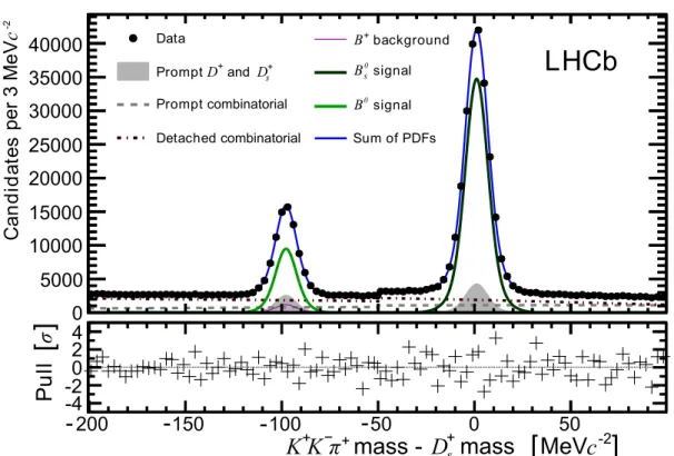
Can d id at es perS3SMe V c -2 Data PromptScombinatorial DetachedScombinatorial PromptSD s +and D+ background + B 0 signal s B 0 signal B SumSofSPDFs -2massSSSSMeVc
s +massS- D
π
K K
+ - +Figure 4: Distribution of measured K+K−π+ mass, where the known mass of the D+s has been subtracted. Black points show the data, and the various lines overlay the result of the fit. The small step at −50 MeVc−2 is the result of differences in tagging efficiency for the B0s and B0 hypotheses.
and n > 0.56), and the tagging result (even and odd). Seven categories of signal and background are assigned component probability density functions (PDFs) whose fractions and shape parameters are left free in the fits to the data. The backgrounds are categorized in terms of their shapes in the mass and decay-time observables. Using the M (K+K−π+) distribution we separate out peaking D(s)+ components from combinatorial background components. Each of these categories can be further divided into two based on their decay-time shape. We use the term “prompt” to describe fake candidates containing particles exclusively produced in the primary pp interaction, and the term “detached” for candidates that contain at least one daughter of a secondary decay and which therefore tend to exhibit a significantly larger lifetime. Candidates for the signal B-decays of interest must be both detached and peaking. The signal-like decays are usually grouped together in the fit; however, we separate the specific background contribution of B+ within the D+ peak and fit that directly. These components are shown in together in Fig. 4 and separately in different M (K+K−π+) regions in Figs. 5 and 6. Each mass PDF is a Gaussian function or a Chebychev polynomial (Fig. 4), and each background decay-time PDF is a simple
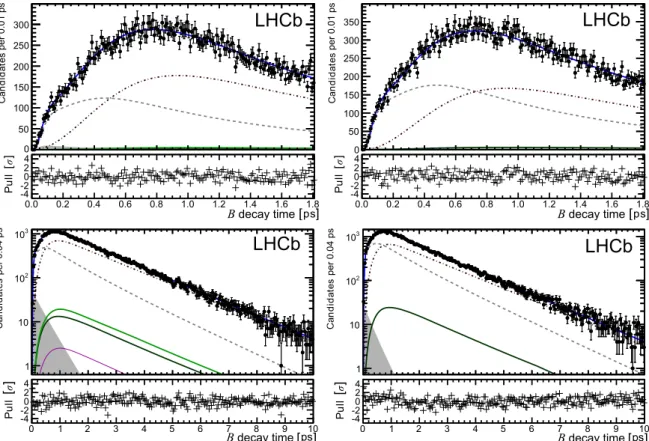
CorrectedgPropergTimeg/gps 0.0 0.2 0.4 0.6 0.8 1.0 1.2 1.4 1.6 1.8 0 50 100 150 200 250 300 massgsidebandgregion π t<1.8ps,gmiddlegkk 0.0 0.2 0.4 0.6 0.8 1.0 1.2 1.4 1.6 1.8 -4 -20 2 ps σ Pu ll 4 [ [ [ [ Bgdecaygtime Can d id at es perg0.01gps LHCb CorrectedgPropergTimeg/gps 0.0 0.2 0.4 0.6 0.8 1.0 1.2 1.4 1.6 1.8 0 50 100 150 200 250 300 350 massgsidebandgregion π t<1.8ps,ghighgkk 0.0 0.2 0.4 0.6 0.8 1.0 1.2 1.4 1.6 1.8 -4 -20 2 ps σ Pu ll 4 [ [ [ [ Bgdecaygtime Can d id at es perg0.01gps LHCb CorrectednPropernTimen/nps 0 1 2 3 4 5 6 7 8 9 10 1 10 2 10 3 10 massnsidebandnregion π middlenkk 0 1 2 3 4 5 6 7 8 9 10 -4 -20 2 4 Can d id at es ps σ Pu ll Bndecayntime pern0.04nps LHCb CorrectednPropernTimen/nps 0 1 2 3 4 5 6 7 8 9 10 1 10 2 10 3 10 massnsidebandnregion π highnkk 0 1 2 3 4 5 6 7 8 9 10 -4 -20 2 4 Can d id at es ps σ Pu ll Bndecayntime pern0.04nps LHCb
Figure 5: Measured B decay-time distribution, overlaid with projections of the fit, for background-only regions. Top left: a region between the two signal peaks, −80 to −20 MeVc−2 (with respect to the known mass of the D+
s), showing only low decay times. Top right: a region to the right of
the signal peaks 20 to 100 MeVc−2, showing only low decay times. Bottom row: the same on an extended decay-time scale and logarithmic. The legend is the same as in Fig. 4.
exponential with an appropriate acceptance function as previously described (Fig. 6). For the signal decay-time shape we use the model described in Eq. 3, with one instance for each peak. The majority of our sensitivity arises from the mixing asymmetry, whose time-dependent fit in the signal regions is shown in Fig. 7. Any odd/even asymmetry is assumed to be constant as a function of time for prompt backgrounds and for backgrounds that are known not to mix (B+, Λ
b, etc.). Generic detached backgrounds are allowed to have a time-dependent asymmetry varying as an arbitrary quadratic polynomial.
The proportion of B+ → D−µ+(ν, π+, γ) with respect to B0 → D−µ+(ν, π0, γ) is fixed to 11 % with a ±2 % uncertainty, using the ratio of known fragmentation functions and branching fractions [1]. Based on the full LHCb simulation, this ratio is corrected by 25 % to account for differences in the reconstruction and tagging efficiencies, with the full value of this correction taken as a systematic uncertainty. We fix ∆Γs using the result of a recent LHCb analysis [24], and ∆Γd is fixed to zero.
Only the signal mass shapes and the parameters of interest, ∆ms and ∆md, are shared
Corrected<Proper<Time</<ps 0.0 0.2 0.4 0.6 0.8 1.0 1.2 1.4 1.6 1.8 0 50 100 150 200 250
High-n, Odd tagged, t<1.8ps, Ds signal region
ps 0.0 0.2 0.4 0.6 0.8 1.0 1.2 1.4 1.6 1.8 σ Pu ll -4 -20 2 4 LHCb [ [ [ [ Bgdecaygtime Can d id at es perg0.01gps Corrected<Proper<Time</<ps 0.0 0.2 0.4 0.6 0.8 1.0 1.2 1.4 1.6 1.8 0 50 100 150 200 250 Odd<tagged,<t<1.8ps,<Dd<signal<region 0.0 0.2 0.4 0.6 0.8 1.0 1.2 1.4 1.6 1.8 -4 -20 2 4 σ Pu ll B<decay<time ps LHCb Can d id at es per<0.01<ps CorrectedDProperDTimeD/Dps 0 1 2 3 4 5 6 7 8 9 10 10 2 10 3 10 DsDsignalDregion 0 1 2 3 4 5 6 7 8 9 10 -4 -20 2 4 Can d id at es ps σ Pu ll LHCb BDdecayDtime perD0.04Dps CorrectedDProperDTimeD/Dps 0 1 2 3 4 5 6 7 8 9 10 1 10 2 10 3 10 DdDsignalDregion 0 1 2 3 4 5 6 7 8 9 10 -4 -20 2 4 Can d id at es D Dps σ Pu ll LHCb BDdecayDtime perD0.04Dps
Figure 6: Measured B decay-time distribution, overlaid with projections of the fit, for signal regions. Top left: for odd-tags, high-n and a region of ±20 MeVc−2 around the D+s mass peak, showing only low decay times, where Bs0 oscillations can be clearly seen. Top right: for odd-tags and all n for a region of ±20 MeVc−2 around the D+ mass peak, showing only low decay times. Bottom row: for both tags and all n for regions of ±20 MeVc−2 around the D+
s (left) and D+
between the two subsamples in n, which are fitted simultaneously. The goodness of the fit is verified with a local density method [25], which finds a p-value of 19.6 %.
6
Fit results and systematic uncertainties
Table 1 gives the fitted values for some important quantities. In principle the signal lifetimes are also measured, but these have very large systematic uncertainties and so no results are quoted. The systematic uncertainties on ∆ms and ∆md are first discussed before the final results are given.
Several sources of systematic uncertainty on the main measured quantities, ∆ms and ∆md, are considered, as summarized in Table 2. The majority of the systematic uncertainties are obtained from the data.
• The k-factor: the k-factor correction is a simulation-based method, and so differences between the simulation and reality that modify the visible and invisible momenta potentially invalidate the correction. Such differences could for example be in D∗∗ branching fractions or form factors. Large-scale pseudo-experiment studies are combined with full simulations to vary these underlying distributions within their uncertainties and examine biases produced on the fitted ∆m values. Small relative uncertainties are found, 0.3 % for ∆ms and 1.0 % for ∆md, representing the ultimate limit of this technique without further knowledge of the various sub-decays.
• Detector alignment: momentum scale, decay-length scale, and track position un-certainties arise from known alignment unun-certainties and result in variations in reconstructed masses and lifetimes as functions of decay opening angle. These
un-CorrectedaProperaTimea/aps 0.0 0.5 1.0 1.5 2.0 2.5 3.0 3.5 4.0 4.5 5.0 A sy m m et ry -0.20 -0.15 -0.10 -0.05 -0.00 0.05 0.10 0.15 0.20 Ds signal region ps 0.0 0.5 1.0 1.5 2.0 2.5 3.0 3.5 4.0 4.5 5.0 σ Pu ll -4 -20 2 4
LHCb
Bndecayntime CorrectednPropernTimen/nps 0 1 2 3 4 5 6 7 8 9 10 A sy m m et ry -0.4 -0.3 -0.2 -0.1 -0.0 0.1 0.2 0.3 0.4 Dd signal region ps 0 1 2 3 4 5 6 7 8 9 10 σ Pu ll -4 -20 2 4LHCb
BAdecayAtime Figure 7: Tagged (mixing) asymmetry, (N+− N−)/(N++ N−), as a function of B decay time.The left plot shows the asymmetry for events for a region of ±20 MeVc−2 around the Ds+ mass peak, and the right plot shows the corresponding asymmetry around the D+ mass peak. The black points show the data and the curves are projections of the fitted PDF. On the left plot the fast oscillations of Bs0 are gradually washed out by the increasingly poor decay-time resolution.
certainties have been studied using detector survey data and various control modes; they are well determined and small in comparison to the statistical uncertainties [26]. • Values of ∆Γ: The quantities ∆Γd and ∆Γs are nominally constant in our fits. When
they are varied, within ±5 % for ∆Γd (chosen to well-cover the experimental range given the lack of information on its sign [1]) and within the known uncertainty on ∆Γs [24], our result is only marginally affected.
• Model bias: a correction has been made for the 1 % residual frequency bias seen in full simulation studies, as discussed in Sec. 4. This is taken directly from simulation and half of the correction is assigned a systematic uncertainty.
• Signal proper-time model: the fit is repeated with two different time-resolution models. (a) When the resolution is parameterized as a function of true rather than measured decay time, using full numerical convolution, a (0.09, 0.002) ps−1 variation is seen in (∆ms, ∆md). (b) When a time-independent (average) resolution is used, a 0.001 ps−1 variation is seen in ∆md (this method is not applicable to the measurement of ∆ms due to many factors; crucially, within the time frame of any single B0
s oscillation the decay time resolution worsens by an appreciable fraction of the oscillation period, seen in Figs. 3 and 7). With other modifications to the signal model (resolutions and acceptances) a larger variation in ∆md of 0.007 ps−1 is found.
• Other models and binning: the order of the Chebychev polynomial is varied, Crystal Ball functions are used for the mass peak shapes, and the background parameteriza-tions and the binning schemes are varied. Out of these modificaparameteriza-tions, the binning
Table 1: A selection of fitted parameter values, for which statistical uncertainties only are given. The Bs0 signal fraction includes contributions from any detached D+s production. When the omitted fractions (of combinatorial background components) are included, the total fraction sums to unity within each n region separately.
Quantity Normalized mass region
Low-n High-n
Fit fraction of:
- Bs0 signal 0.3247±0.0029 0.3604±0.0023 - B0 signal 0.0781±0.0017 0.0968±0.0022 - prompt Ds+ 0.0410±0.0026 0.0444±0.0018 - prompt D+ 0.0196±0.0018 0.0311±0.0024 Mistag probability ω: - Bs0 signal 0.347±0.054 0.333±0.021 - B0 signal 0.3567±0.0063 0.3319±0.0065 Total candidates 368,965 225,880
scheme has the largest effect. Resulting uncertanties of 0.05 ps−1 and 0.001 ps−1 are assigned to ∆ms and ∆md, respectively.
• Assumptions on B+ decays: The ∆m
dmeasurement is sensitive to χd, the integrated mixing probability, which in turn is sensitive to the non-mixing B+-background. We hold constant several B+-background parameters in the baseline fit, determined from the full simulation. Many features of the B+ background fit are varied to evaluate systematic variations, including the fraction, the lifetime, and the corrections for relative tagging performance. The largest uncertainty arises from tagging performance corrections and for this a 0.008 ps−1 uncertainty is assigned to ∆md. It is possible to leave one or more of these parameters free during the fit, but the loss in statistical precision is prohibitive.
For cross-checks the data are split by LHCb magnet polarity and LHCb trigger strategies; no variations beyond the expected statistical fluctuations are observed. We obtain
∆ms = (17.93 ± 0.22 (stat) ± 0.15 (syst)) ps−1, ∆md= (0.503 ± 0.011 (stat) ± 0.013 (syst)) ps−1.
To obtain a measure for the significance of the observed oscillations, the global likelihood minimum for the full fit is compared with the likelihood of the hypotheses corresponding to the edges of our search window (∆m = 0 or ∆m ≥ 50 ps−1). Both would result in almost flat asymmetry curves (cf. Fig. 7) corresponding to no observed oscillations. We reject the null hypothesis of no oscillations by the equivalent of 5.8 standard deviations for B0
s oscillations and 13.0 standard deviations for B0 oscillations.
Table 2: Sources of systematic uncertainty on ∆msand ∆md. “Simulation” implies a combination
of full LHCb simulation and pseudo-experiment studies.
Source of uncertainty Method Systematic uncertainty
∆ms [ps−1] ∆md[ps−1]
k-factor Simulation 0.06 0.0052
Detector alignment Calibration 0.03 0.0008
Values of ∆Γ Data refit n/a 0.0004
Model bias Simulation 0.09 0.0055
Signal proper-time model Data refit 0.09 0.007
Other models and binning Data refit 0.05 0.001
B+ (B, efficiency, tagging) Data refit n/a 0.008
7
Fourier analysis
The full fit as described above was performed in the time domain, but measurement of the mixing frequency can also be made directly in the frequency domain as a cross-check, using well-established Fourier transform techniques [27–29]. The cosine term in Eq. 3 has a different sign for the odd and even samples, where the lifetime, acceptance, and other features are shared; this simplifies the analysis in the frequency domain. Any Fourier components not arising from mixing are suppressed by subtracting the odd Fourier spectrum from the even spectrum and no parameterizations of the background shapes, signal shapes, or decay-time resolution are required, allowing a model-independent measurement of the mixing frequencies. We search for the ∆ms peak in the subtracted Fourier spectrum, shown in Fig. 8. Extensive fast simulation pseudo-experiments have shown that the value of ∆ms is obtained reliably and with a reasonable precision using this method; however ∆md is heavily biased and has a large uncertainty, and so a result is not quoted. Since residual components of the Fourier spectrum are of much lower frequency than the ∆ms component, and several complete oscillation periods of ∆ms are observable, the search for a spectral peak is relatively free from complications. For ∆md, however, the relatively low frequency is similar to that of many other features of the data, and only a single oscillation period is observed; therefore the determination of ∆md is difficult with this simple model-independent approach.
5 10 15 20 30 Frequency,ω ps− 1 −200 −150 −100 −50 0 50 100 massCbinC( 25CMeV c − 2wid ths) MeV c − 2 LHCb [ [ [ [ 25 π K K + + -0 200 400 600 800 1000 Int ensi ty ,arb . 17.0 17.5 18.0 18.5 19.0 Frequency, ω ps[ −1[ LHCb
Figure 8: Result of using Fourier transforms to search for the ∆ms-peak. The image on the left
is constructed from bins of the K+K−π+ mass which are 25 MeVc−2 in width, analysed in steps of 5 MeVc−2 such that a smooth image is produced. The colour scale (blue-green-yellow-red) is an arbitrary linear representation of the signal intensity; dark blue is used for zero and below. The vertical dashed line is drawn at 18.0 ps−1. The apparent double-peak structure is an artifact of this image. On the right a slice around the Ds+ mass region shows only the peak as used to measure the central value and rms width.
Taking the spectrum for events in a 25 MeVc−2 bin around the Ds+ mass, we find a clear and separated peak (Fig. 8, right). The rms width of the peak is 0.4 ps−1, around a peak value of 17.95 ps−1; the rms can be used as a model-independent proxy for the statistical uncertainty. To further evaluate the expected statistical fluctuation in the peak value, we perform a large set of fast simulation pseudo-experiments taking the result of the multivariate fit as a model for signal and background. The uncertainty found from the simulation studies is 0.32 ps−1, slightly smaller than given by the rms. We report ∆ms= (17.95 ± 0.40 (rms) ± 0.11 (syst)) ps−1, in order to be model-independent. Systematic uncertainties arise from the detector alignment and the k-factor correction method, common to both measurement techniques, as quantified previously in Sec. 6.
8
Conclusion
The mixing frequencies for neutral B mesons have been measured using flavour-specific semileptonic decays. To correct for the momentum lost to missing particles, a simulation-based kinematic correction, known as the k-factor, was adopted. Two techniques were used to measure the mixing frequencies: a multidimensional simultaneous fit to the K+K−π+ mass distribution, the decay-time distribution, and tagging information; and a simple Fourier analysis. The results of the two methods were consistent, with the first method being more precise. We obtain
∆ms = (17.93 ± 0.22 (stat) ± 0.15 (syst)) ps−1, ∆md= (0.503 ± 0.011 (stat) ± 0.013 (syst)) ps−1.
We reject the hypothesis of no oscillations by 5.8 standard deviations for B0
s and 13.0 standard deviations for B0. This is the first observation of B0
s-B0s mixing to be made using only semileptonic decays.
Acknowledgements
We express our gratitude to our colleagues in the CERN accelerator departments for the excellent performance of the LHC. We thank the technical and administrative staff at the LHCb institutes. We acknowledge support from CERN and from the national agencies: CAPES, CNPq, FAPERJ and FINEP (Brazil); NSFC (China); CNRS/IN2P3 and Region Auvergne (France); BMBF, DFG, HGF and MPG (Germany); SFI (Ireland); INFN (Italy); FOM and NWO (The Netherlands); SCSR (Poland); MEN/IFA (Romania); MinES, Rosatom, RFBR and NRC “Kurchatov Institute” (Russia); MinECo, XuntaGal and GENCAT (Spain); SNSF and SER (Switzerland); NAS Ukraine (Ukraine); STFC (United Kingdom); NSF (USA). We also acknowledge the support received from the ERC under FP7. The Tier1 computing centres are supported by IN2P3 (France), KIT and BMBF (Germany), INFN (Italy), NWO and SURF (The Netherlands), PIC (Spain), GridPP (United Kingdom). We are thankful for the computing resources put at our
disposal by Yandex LLC (Russia), as well as to the communities behind the multiple open source software packages that we depend on.
References
[1] Particle Data Group, J. Beringer et al., Review of particle physics, Phys. Rev. D86 (2012) 010001.
[2] O. Schneider, for the Particle Data Group, B0 - ¯B0 mixing, in [1].
[3] ARGUS collaboration, H. Albrecht et al., Observation of B0 - ¯B0 mixing, Phys. Lett. B192 (1987) 245.
[4] CDF collaboration, A. Abulencia et al., Observation of Bs0 - ¯Bs0 oscillations, Phys. Rev. Lett. 97 (2006) 242003, arXiv:hep-ex/0609040.
[5] LHCb collaboration, R. Aaij et al., Precision measurement of the B0 s–B
0
s oscilla-tion frequency ∆ms in the decay B0s → Ds+π
−, New J. Phys. 15 (2013) 053021, arXiv:1304.4741.
[6] LHCb collaboration, R. Aaij et al., Opposite-side flavour tagging of B mesons at the LHCb experiment, Eur. Phys. J. C72 (2012) 2022, arXiv:1202.4979.
[7] LHCb collaboration, R. Aaij et al., Measurement of the B0–B0 oscillation frequency ∆md with the decays B0 → D−π+ and B0 → J/ψK∗0, Phys. Lett. B719 (2013) 318, arXiv:1210.6750.
[8] LHCb collaboration, A. A. Alves Jr. et al., The LHCb detector at the LHC, JINST 3 (2008) S08005.
[9] M. Adinolfi et al., Performance of the LHCb RICH detector at the LHC, Eur. Phys. J. C73 (2013) 2431, arXiv:1211.6759.
[10] A. A. Alves Jr et al., Performance of the LHCb muon system, JINST 8 (2013) P02022, arXiv:1211.1346.
[11] R. Aaij et al., The LHCb trigger and its performance in 2011, JINST 8 (2013) P04022, arXiv:1211.3055.
[12] Sj¨ostrand, Torbj¨orn and Mrenna, Stephen and Skands, Peter, PYTHIA 6.4 physics and manual, JHEP 05 (2006) 026, arXiv:hep-ph/0603175.
[13] I. Belyaev et al., Handling of the generation of primary events in Gauss, the LHCb simulation framework, Nuclear Science Symposium Conference Record (NSS/MIC) IEEE (2010) 1155.
[14] D. J. Lange, The EvtGen particle decay simulation package, Nucl. Instrum. Meth. A462 (2001) 152.
[15] P. Golonka and Z. Was, PHOTOS Monte Carlo: a precision tool for QED corrections in Z and W decays, Eur. Phys. J. C45 (2006) 97, arXiv:hep-ph/0506026.
[16] Geant4 collaboration, J. Allison et al., Geant4 developments and applications, IEEE Trans. Nucl. Sci. 53 (2006) 270; Geant4 collaboration, S. Agostinelli et al., Geant4: a simulation toolkit, Nucl. Instrum. Meth. A506 (2003) 250.
[17] M. Clemencic et al., The LHCb simulation application, Gauss: design, evolution and experience, J. Phys.: Conf. Ser. 331 (2011) 032023.
[18] M. Grabalosa, Flavour tagging developments within the LHCb experiment, CERN-THESIS-2012-075.
[19] N. T. Leonardo, Analysis of Bs flavor oscillations at CDF, FERMILAB-THESIS-2006-18, 2006.
[20] M. S. Anzelc, Study of mixing at the DØ detector at Fermilab using the semi-leptonic decay Bs→ DsµνX, FERMILAB-THESIS-2008-07, 2008.
[21] T. Bird, Towards measuring B mixing in semileptonic decays at LHCb, CERN-THESIS-2011-184, 2011.
[22] R. Brun and F. Rademakers, Root- an object oriented data analysis framework, vol. 389 of AIHENP’96 Workshop, Lausanne, pp. 81–86, Sep, 1996. doi: 10.1016/S0168-9002(97)00048-X.
[23] W. Verkerke and D. Kirkby, The RooFit toolkit for data modeling, in 2003 Con-ference for Computing in High-Energy and Nuclear Physics (CHEP 03), (La Jolla, California, USA), March, 2003. arXiv:physics/0306116.
[24] LHCb collaboration, R. Aaij et al., Measurement of CP -violation and the Bs0-meson decay width difference with B0
s → J/ψK+K
− and B0
s → J/ψπ+π
− decays, Phys. Rev. D87 (2013) 112010, arXiv:1304.2600.
[25] M. Williams, How good are your fits? Unbinned multivariate goodness-of-fit tests in high energy physics, JINST 5 (2010) P09004, arXiv:1006.3019.
[26] J. Amoraal et al., Application of vertex and mass constraints in track-based alignment, Nucl. Instrum. Meth. A712 (2013) 48, arXiv:1207.4756.
[27] J. B. J. Fourier, Th´eorie analytique de la chaleur, Chez Firmin Didot, p`ere et fils (1822).
[29] H. Moser and A. Roussarie, Mathematical methods for B0 anti-B0 oscillation analyses, Nucl. Instrum. Meth. A384 (1997) 491.