Dynamic airline scheduling and robust airline schedule de-peaking

Dynamic Airline Scheduling and

Robust Airline Schedule De-Peaking

by

Hai Jiang

B.S., Tsinghua University (2001)

M.S., Massachusetts Institute of Technology (2003)

Submitted to the Department of Civil and Environmental Engineering

in partial fulfillment of the requirements for the degree of

Doctor of Philosophy in Transportation

at the

MASSACHUSETTS INSTITUTE OF TECHNOLOGY

September 2006

@

Massachusetts Institute of Technology 2006. All rights reserved.

A uthor ... L a ... . . . .... .,... s ...

Departmet of - ivil and Environmental Engineering

August 11, 2006

Certified by...

Accepted by

MAssA idisisisn

Chairman,

OF TECHNOLOGY

DEC

_L

₅

₂₀₀₆

.. ..

...

..

..

Cynthia Barnhart

Professor of Civil and Environmental Engineering

Thesis Supervisor

j-0 1.

... _{r... . C.o... ...}

.

1.

_{u . ...}

Andre 1-4ittle Department Committee on

Graduate Students

Dynamic Airline Scheduling and

Robust Airline Schedule De-Peaking

by

Hai Jiang

Submitted to the Department of Civil and Environmental Engineering on August 11, 2006, in partial fulfillment of the

requirements for the degree of Doctor of Philosophy in Transportation

Abstract

Demand stochasticity is a major challenge for the airlines in their quest to produce profit maximizing schedules. Even with an optimized schedule, many flights have empty seats at departure, while others suffer a lack of seats to accommodate pas-sengers who desire to travel. Recognizing that demand forecast quality for a par-ticular departure date improves as the date comes close, we tackle this challenge by developing a dynamic scheduling approach that re-optimizes elements of the flight schedule during the passenger booking period. The goal is to match capacity to demand, given the many operational constraints that restrict possible assignments. We introduce flight timing as a dynamic scheduling mechanism and develop a re-optimization model that combines both flight re-timing and flight re-fleeting. Our re-optimization approach, re-designing the flight schedule at regular intervals, utilizes information from both revealed booking data and improved forecasts available at later re-optimizat ions. Experiments are conducted using data from a major U.S. airline. We demonstrate that significant potential profitability improvements are achievable using this approach.

We complement this dynamic re-optimization approach with models and algo-rithms to de-peak existing hub-and-spoke flight schedules so as to maximize future dynamic scheduling capabilities. In our robust de-peaking approach, we begin by solving a basic de-peaking model to provide a basis for comparison of the robust de-peaked schedule we later generate. We then present our robust de-peaking model to produce a schedule that maximizes the weighted sum of potentially connecting

itineraries and attains at least the same profitability as the schedule produced by the

basic de-peaking model. We provide several reformulations of the robust de-peaking model and analyze their properties. To address the tractability issue, we construct a restricted model through an approximate treatment of the profitability requirement.

The restricted model is solved by a decomposition based solution approach involving a variable reduction technique and a new form of column generation. We demon-strate, through experiments using data from a major U.S. airline, that the schedule generated by our robust de-peaking approach achieves improved profitability.

Acknowledgments

I am fortunate and blessed to have Professor Cynthia Barnhart as my advisor during

my doctoral study. I am deeply grateful to Cindy for her constant encouragement and tremendous support through the years. She has given me the widest freedom to pursue my research directions, and provided me the most valuable advice on how to enhance this work. She also showed great care and understanding to me and always stated that the student's interests are primary while the advisor's are secondary. Cindy made herself available to me during weekends and evenings. We sometimes even talked over the phone about research when she was driving between Boston and Vermont. She is indeed a great advisor.

I would like to thank my doctoral committee members, Professor Nigel Wilson

and Professor John-Paul Clarke for their insightful comments and suggestions.

I would like to thank my colleagues in the Large-Scale Optimization Group for

their friendship. I would like to extend my thanks to Ginny Siggia and Maria Marang-iello for their wonderful assistance in all matters.

Many thanks go to the United Parcel Service and the Sloan Foundation for pro-viding financial support for my doctoral study.

Finally, I want to thank my family for their love and confidence in my ability to

Contents

1 Introduction 17

1.1 M otivation . . . . 17

1.2 Research Summary . . . . 19

1.2.1 Dynamic Airline Scheduling . . . . 20

1.2.2 Robust Airline Schedule De-Peaking . . . . 21

1.3 Thesis Contributions . . . . 22

1.4 Thesis Organization . . . . 23

2 Dynamic Airline Scheduling 25 2.1 Introduction . . . . 25

2.2 Airline Route Networks and Flight Schedules . . . . 28

2.2.1 Linear Networks . . . . 28

2.2.2 Hub-and-Spoke Networks with Banked Flight Schedules . . . . 29

2.2.3 Moving Toward De-Peaked Schedules . . . . 31

2.2.4 De-Peaking in Practice . . . . 33

2.3 Opportunities in a De-Peaked Hub-and-Spoke Network . . . . 36

2.4 Modeling Architecture . . . . 37

2.4.1 Service Guarantee to Previously Booked Passengers . . . . 40

2.4.2 Frequency and Timing of Re-Optimization Points . . . . 41

2.4.3 Flow Charts . . . . 41

2.5 Mathematical Models . . . . 42

2.5. -1 Term inology . . . . 43

2.5.3 Passenger Mix Model . . . .

2.5.4 Re-Optimization Model . . . .

2.6 Solution Approach and Computational Experiences . . . .

2.7 Case Study 1: Daily Schedules . . . .

2.7.1 Assumptions on Unconstrained Demand and Forecast

Q

2.7.2 R esults . . . .

2.7.3 Quality of the Original Schedule . . . .

2.8 Case Study 2: Weekly Schedules . . . .

2.8.1 Schedule Generation . . . .

2.8.2 Unconstrained Demand and Forecast Quality . . . . . 2.8.3 R esults . . . .

2.8.4 Quality of the Original Schedule . . . .

2.9 O ther Issues . . . .

2.9.1 Effects of Dynamic Scheduling on Aircraft Maintenance

ing, Crew Scheduling, and Passenger Itineraries . . . .

2.9.2 Applicability of Dynamic Scheduling to Other Airlines

2.10 Sum m ary . . . .

3 Robust Airline Schedule De-Peaking

3.1 Introduction . . . .

3.2 The Schedule De-Peaking Problem and Related Literature

3.3 Basic De-Peaking Model . . . . 3.4 Robust De-Peaking Model . . . . 3.4.1 Formulation 1 . . . . 3.4.2 Formulation 2 . . . . 3.4.3 Formulation 3 . . . . 3.4.4 Formulation 4 . . . . 3.4.5 Additional Insights . . . .

3.5 Restricted Robust De-Peaking Model . . . .

3.6 Solution Approach . . . . 95 . . . . 95 . . . . 97 . . . . 99 . . . . 102 . . . . 105 . . . . 107 . . . . 110 . . . . 114 . . . . 121 . . . . 126 . . . . 129 44 48 57 58 59 66 74 79 79 80 86 87 87 88 89 92 uality

Rout-3.7 Computational Experiences . . . 132

3.7.1 Comparison of the LP relaxations . . . 133

3.7.2 Searching for Integer Solutions . . . 134

3.8 Case Study . . . 137

3.8.1 Resulting Schedule Characteristics . . . 137

3.8.2 Comparison of Dynamic Scheduling Results . . . 139

3.8.3 Quality of the Robust Schedule . . . 140

3.9 Sum m ary . . . . 141

List of Figures

1-1 Histogram of load factors for all flights operated by a major U.S. airline

in a 4-week period . . . . 2-1 Departure and arrival activities at hub in a banked schedule . . . . .

2-2 Departure and arrival activities at hub in a de-peaked schedule . . . .

2-3 2-4 2-5 2-6 2-7 2-8 2-9 2-10 2-11 2-12 2-13 2-14 2-15 2-16 2-17 19 30 32 Original schedule . . . . 37

Re-timing creates new connecting itineraries . . . . 37

Original schedule . . . . 38

New schedule . . . . 38

Dynamic scheduling process . . . . 38

Static case . . . . 42

Dynamic scheduling case . . . . 43

Flight copy indices . . . . 54

Cumulative demand . . . . 62

Cumulative demand as a fraction of total demand . . . . 62

Forecast quality (scatter plot) . . . . 63

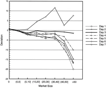
Average absolute deviation in each market group . . . . 64

Average deviation in each market group . . . . 64

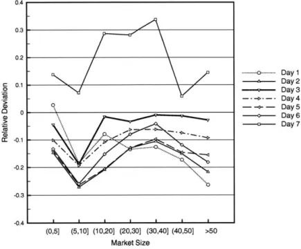
Average absolute relative deviation in each market group . . . . 65

Average relative deviation in each market group . . . . 65 2-18 Profit increase as a function of total number of re-timed flights

cast A ) . . . .

2-19 Achieved profit increase as a function of total number of re-timed flights

(Forecast A ) . . . . 77

2-20 Two types of new connecting itineraries . . . . 78

2-21 Daily mean load factor and quantiles of the load factor histogram for a major U.S. airline in a 4-week period. Days 1, 8, 15, and 22 correspond to Saturdays . . . . 80

2-22 Cumulative demand curves . . . . 82

2-23 Cumulative demand curves as a fraction of total demand . . . . 82

2-24 Forecast quality (scatter plot) . . . . 83

2-25 Average absolute deviation in each market group . . . . 84

2-26 Average deviation in each market group . . . . 84

2-27 Average absolute relative deviation in each market group . . . . 85

2-28 Average relative deviation in each market group . . . . 85

2-29 Histograms and cumulative percentages of flight load factors for two major US hub-and-spoke carriers. The figure on the top is based on 2004 data and the one on the bottom is based on 2003 data. Source: PODS Consortium, ICAT, MIT (2006) . . . . 93

3-1 Illustration of connection variables . . . 105

3-2 Example to illustrate formulation strength . . . 109

3-3 Illustration of Formulation 4 . . . 115

3-4 Flight copy indices . . . . 123

3-5 Connection variables formed by flight copies of 11 and 12 . . . . . . 124

3-6 Solution algorithm for the robust de-peaking model . . . 131

3-7 Number of departures (negative values) and arrivals (positive values) at hub under the banked schedule . . . . 142

3-8 Number of departures (negative values) and arrivals (positive values) at hub under the de-peaked schedule obtained with the basic de-peaking m odel . . . 142

3-9 Distributions of passenger connection times based on actual passenger data under Schedule A and results from PMM under Schedules A, B, and C . . . . 143

List of Tables

2.1 Default display on the websites of major airlines and leading Internet air ticket retailers (obtained by visiting each website on March 6, 2006) 34

2.2 Itinerary prior to re-timing . . . . 40

2.3 Itinerary after re-timing . . . . 40

2.7 Connection times between flight copies . . . . 56

2.8 Problem sizes and solution times . . . . 58

2.9 Fleet composition and capacity . . . . 59

2.10 Daily operating results under two forecast scenarios (in dollars) . . . 67

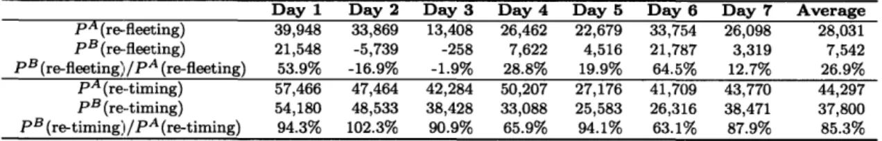
2.11 Comparison between re-fleeting and re-timing under Forecast A (in dollars) . . . . 68

2.12 Comparison between re-fleeting and re-timing under Forecast B (in dollars) . . . . 69

2.13 The ratio of profit increase under Forecast B to that under Forecast A when each mechanism is applied alone . . . . 69

2.14 Passenger and revenue (in dollars) statistics under Forecast A when re-fleeting and re-timing are applied alone . . . . 71

2.15 Profit increase when limiting the number of re-timed flights under Fore-cast B . . . . 73

2.16 Statistics on Type I and Type II passengers (MinCT = 25 minutes and MaxCT = 180 minutes) . . . . 74

2.17 Re-timing decisions for frequently re-timed flights . . . . 76

2.18 Daily operating results under two forecast scenarios (in dollars) . . . 86

2.20 Connecting passenger statistics on domestic itineraries at the 30 largest

U.S. airport based on number of domestic passengers enplaned . . . . 91

2.21 Connecting passenger statistics on domestic itineraries for major U.S.

airlines at hub or major airports . . . . 94

3.3 Number of constraints needed to model the relationship between f1k,

variables and hp variables in each formulation. . . . . 120

3.4 Comparison of LP relaxations of the full problem across formulations

(Z1 = 126, 217) . . . . 134

3.5 Summary statistics of hp variables in the restricted de-peaking model

when flk, variables are fixed to corresponding values in the basic

de-peaking solution . . . 135

3.6 Branch-and-bound results for Formulations 1-R through 4-R on the

initial Restricted Master Problem . . . . 136

3.7 Resulting schedule characteristics (ZL = 129,142) . . . . 138 3.8 Comparisons between Schedule B and Schedule C when averaged over a

week's operation (in dollars). The number of re-timed flights is limited to 100 and the number of re-fleeted flights is unconstrained . . . 140

3.9 Comparisons between Schedule B and Schedule C for each individual

day in a week's operation (in dollars). The number of re-timed flights

is limited to 100 and the number of re-fleeted flights is unconstrained 144

3.10 Re-timing decisions for frequently re-timed flights in Schedule C . . . 145

3.11 Flights frequently and consistently re-timed in both Schedule B and

Chapter 1

Introduction

1.1

Motivation

It has been a major challenge for airlines to design a flight schedule (timetable and fleeting) to match fluctuating passenger demand. The flight schedule, that is, the supply side of the passenger air transportation system, has to be determined well in advance due to contractual and operational requirements in the industry. Examples of the schedule planning process can be found in Goodstein (1997), Jarrah (2000), Barnhart et al. (2002), and Frank et al. (2005). The steps and timelines of the schedule planning process may differ slightly from one airline to another, yet it typically starts 12 months prior to departure and lasts approximately 9 months. To generate a schedule that has the most revenue potential, the airline's scheduling department compiles input data to the planning process that reflects a macro-forecast of the economy, the airline's strategic objectives, forecasted passenger demands, average fares, available resources (aircraft, personnel, gates), and so on. Then, the flight schedule is constructed and published through different distribution channels. Despite the fact that scheduling decisions are made at a time when demand is highly uncertain, the schedule is anticipated to be carried out on the date of departure.

In the booking period, that is, the time between the schedule being published and the departure date, airlines employ sophisticated revenue management techniques to sell as many seats as possible in the flight schedule, while maximizing revenue. In peak

demand situations, prices are raised, thereby reserving the scarce seats for high fare passengers. When demands are low, prices are reduced to stimulate bookings. Hence, revenue management systems help to shape demand to fit the fixed supply of seats in the schedule. Nevertheless, no matter how sophisticated these systems are, the stochastic nature of passenger demand still results in many flight legs having empty seats upon departure, while others suffer a lack of seats to accommodate passengers who desire to travel. Figure 1-1 shows the histogram of load factors (LFs) (the ratio of the number of paid passenger seats on a flight to the seating capacity of the flight) for all flights operated by a major U.S. airline in a month. The load factors range widely, with a mean of 0.76. The quantiles of the histogram show that more than 25% of the flights are highly demanded and are sold close to capacity (LFs are greater than

0.93), while at the same time another 25% of the flights have significant numbers of

empty seats (LFs are less than 0.66, that is, about 1 out of every 3 seats remain unsold at the time of departure). The imbalanced load factors across flight legs indicate that the actual demand at the departure date is far from being accurately captured by the demand forecasts used in developing the schedule. If those empty seats appeared on flight legs with excess demand, significant revenue gains would be possible.

Because forecast quality improves dramatically as the time of departure approaches (see Berge and Hopperstad 1993, Feldman 2000, Bish et al. 2004, and Sherali et al.

2005), an interesting question is how an airline can utilize improved demand forecasts

to re-optimize the original schedule and move excess capacity to flight legs with a shortage of capacity. We focus on developing mechanisms to be used in matching supply and (fluctuating) demand, by making only small changes to the schedule so as to minimize the complication in operations. In doing so, capacity will be shifted from flight legs with expected excess capacity to those with expected capacity short-falls, and hence, forecast quality will play a central role in making wise capacity shift decisions. Of particular interest is how the re-optimized schedule performs when vary-ing degrees of forecast quality are available. After evaluatvary-ing the effects of schedule re-optimization, we consider the question of how to design a schedule that allows maximal flexibility for adjustment during the booking process in response to

unex-20.0 Mean 0.769986 Std Deviation 0.219068 17.5 Minimum 0.007937 Maximum 1 15.0 10th Percentile 0.44 Lower Quartile 0.66 Median 0.840708 12.5 Upper Quartile 0.935484 e 90th Percentile 0.982301 r C 10.0 e n t 7.5 5.0 2.5 0 0.000 0.100 0.200 0.300 0.400 0.500 0.600 0.700 0.800 0.900 1.000 LF

Figure 1-1: Histogram of load factors for all flights operated by a major U.S. airline in a 4-week period

pected levels of demand. Because this is a largely unexplored question, we begin

by recognizing the need for metrics to gauge schedule flexibility, and then the need

for new models and algorithms to determine schedules that maximize these schedule flexibility metrics, while simultaneously increasing realized schedule profitability.

1.2

Research Summary

In this thesis we organize the questions mentioned in the previous section into two re-search topics: one focuses on schedule re-optimization, or dynamic airline scheduling; and the other aims at developing robust schedules, that is, flexible schedules achiev-ing maximal profitability when the schedules are allowed to be altered dynamically as passenger demands materialize during the booking process. We focus on the effects of dynamic and robust scheduling in airline networks in which one or more hubs are

de-peaked, that is, the set of incoming and outgoing flights are interspersed, unlike peaked or banked hubs in which flight leg arrivals typically occur first, followed by

inac-tivity between arrival and departure banks allows connecting passengers to disembark from their aircraft, walk to their connecting gates and embark on their departing air-craft. The recent trend of schedule de-peaking by hub-and-spoke carriers provides us with an opportunity to develop and utilize dynamic and robust scheduling approaches that adjust the number of seats in various markets to match passenger demands at departure and maximize final schedule profitability.

1.2.1

Dynamic Airline Scheduling

The concept of dynamic airline scheduling, in which elements of the schedule are re-optimized in the booking period to reflect improved knowledge of passenger de-mands, dates back to the work by Etschmaier and Mathaisel (1984) and Peterson

(1986), where re-fleeting, or aircraft swapping, is proposed as a dynamic scheduling

mechanism. Using improved demand forecasts, the fleeting of flights in the sched-ule are adjusted later in the booking process to match improved demand forecasts. Berge and Hopperstad (1993) are the first to provide an in-depth presentation of this concept, providing implementation and performance evaluation details. Bish et al. (2004) and Sherali et al. (2005) later provide additional insights regarding dynamic re-fleeting approaches.

We begin with a review of the recent trend of schedule de-peaking by legacy hub-and-spoke carriers. Recognizing the high operating costs associated with peaked schedules, many legacy carriers have adopted de-peaked schedules in an attempt to cut costs through increased resource productivity. We observe that, in addition to cutting costs, de-peaked schedules can lead to increased revenues if small flight re-timings are allowed. These re-re-timings alter the set of connecting itineraries serving a market, and therefore, provide a mechanism for increasing the number of seats sold in markets with unexpectedly high demand, without utilizing more aircraft or crew resources. We develop a schedule re-optimization model that combines both flight leg re-fleeting and re-timing. In our dynamic airline scheduling approach, the re-optimization model is used to re-design the flight schedule at regular intervals, utilizing information from both revealed bookings and improved forecasts available

at the time of re-optimization. The re-optimization model is solved by a branch-and-bound method, aided with branching on Special Ordered Sets. Experiments are conducted under two forecast scenarios: one with perfect information and the other with simple averages calculated from historical demands. Two sets of experiments are performed. In the first set, a same-everyday schedule is assumed and experiments are carried out for a week of operations. We determine the resulting profit improve-ments and report the contributions of flight re-fleeting and re-timing when applied alone or jointly. We also study the effect of forecast quality to the benefits of dy-namic scheduling. Because schedule changes, especially flight re-timings, complicate operations, we conduct sensitivity analyses to determine the degradation in schedule profitability when the number of changes are limited. We also evaluate the duration of the passenger connection times for the itineraries newly created through flight leg re-timings. In the second set of experiments, a same-every week schedule is assumed and experiments are carried out on the same weekday in seven consecutive weeks to assess the potential benefit of dynamic scheduling in the absence of day-of-week demand variations.

1.2.2

Robust Airline Schedule De-Peaking

The success of dynamic scheduling not only relies on improved demand forecasts, but also on the amount of flexibility to adjust capacity in the original schedule. In the second part of this thesis, we explore ways to imbed flexibility in the original schedule and increase its robustness. Such a schedule is robust in the sense that it has enhanced capability to handle demand variations through dynamic scheduling.

Expanding on the observations of Berge and Hopperstad (1993) that flight re-fleeting opportunities can be abundant in hub-and-spoke networks, we expend our efforts to identify metrics to measure the amount of flight re-timing opportunities in a schedule. We then develop a two step approach to construct robust de-peaked schedules. In the first step, a basic de-peaking model, ignoring the potential for altering the schedule dynamically during the booking period, is solved to obtain a baseline schedule and its associated profit. In the second step, a robust de-peaking model

is developed to maximize the potential for new connecting itineraries to be created through schedule adjustments in the booking period, while achieving similar profits as the baseline schedule. We present and compare several reformulations of the robust de-peaking model, each with distinct mathematical and computational properties. We next present an approximate model to reduce the size of the problem. The model is solved by branch-and-bound algorithms together with a decomposition approach involving a variable reduction technique and a new form of column generation, which result in dramatically reduced problem sizes, and greatly enhanced tractability. We compare the robust and baseline schedules and report that greater profitability is

achieved by our robust schedules.

1.3

Thesis Contributions

In this thesis, our contributions to the knowledge base of dynamic airline scheduling include:

* We introduce a new dynamic scheduling mechanism, that of flight re-timing, and develop a schedule re-optimization model that integrates both flight re-fleeting and flight re-timing. Experiments are conducted using data from a major U.S. airline.

" We demonstrate that dynamic scheduling improves profitability by 2.5-5%, or $18-36 million annually. We study the effects of forecast quality on these

ben-efits and show that considerable benben-efits remain even when simple forecasts calculated from historical data are used. We also report that the full benefit of re-timing is achieved even when the number of flight legs that are re-timed is strictly restricted.

" We compare and analyze the effectiveness of flight leg re-timing and re-fleeting,

our two dynamic scheduling mechanisms, when applied alone under different forecast scenarios. Flight re-timing demonstrates less sensitivity to the dete-rioration of forecast quality and contributes a larger portion to the potential

benefit of dynamic scheduling.

* We show that benefits remain significant when dynamic scheduling is applied to weekly schedules, in which day-of-week demand variations are explicitly con-sidered in constructing the schedules.

In this thesis, our contributions to the knowledge base of robust scheduling include the following:

" This work represents the first research effort of its kinds in which flexibility is

built into the original schedule to facilitate later application of dynamic schedul-ing.

" We present a mathematical model and several reformulations to achieve this

schedule robustness. By studying the mathematical and computational prop-erties of these reformulations, we devise new solution algorithms and conduct experiments using data from a major U.S. airline. We show that a robust schedule further improves profitability of dynamic scheduling by an additional

1%.

1.4

Thesis Organization

We organize the remainder of this thesis as follows. In Chapters 2 and 3, we study the topics of dynamic airline scheduling and robust schedule de-peaking, respectively. Future research directions extending elements of this thesis are detailed in Chapter 4.

Chapter 2

Dynamic Airline Scheduling

2.1

Introduction

It has been a major challenge for airlines to design a flight schedule, that is, the timetable and the corresponding fleeting on each flight leg, to match fluctuating passenger demand. The flight schedule, defining the supply side of the passenger air transportation system, is designed well in advance, typically six months to one year prior to its implementation, due to contractual and operational requirements in the industry. The design process to generate a schedule that has the maximum profit potential utilizes macro-forecasts of the economy and the airline industry, forecasts of passenger demand, estimates of average fares, and estimates of available resources, such as aircraft, personnel, and gates. The resulting schedule is published through different distribution channels. Despite the fact that scheduling decisions are made at a time when demand is highly uncertain, the flight schedule is intended to remain unchanged once published. More often than not, the published schedule fails to allocate the optimal number of seats, that is, capacity, to where it is needed.

During the booking period, that is, the time between the date the schedule is pub-lished and the departure date, airlines employ different revenue management tech-niques to maximize the schedule's revenue. By increasing fares on highly demanded flights to decrease low fare demands and reducing fares on flights with excess capacity to stimulate travel, revenue management techniques help to smooth demand

varia-tions. Notwithstanding these techniques, the stochastic nature of passenger demand still results in some revenue being lost due to non-optimal allocations of capacity.

To achieve the goal of balancing supply and demand, researchers have started to focus their attention on the supply side and the concept of dynamic airline scheduling was born, that is, the flight schedule is re-optimized during the booking period using improved demand forecast. An early discussion of the concept of dynamic airline scheduling can be found in Etschmaier and Mathaisel (1984) and Peterson (1986). In a survey of aircraft scheduling problems, Etschmaier and Mathaisel (1984) mention dynamic scheduling as an emerging operating philosophy, where the exact schedule could be made as the total demand situation evolves. Peterson (1986) proposes the idea of re-fleeting the schedule during the booking period to better match updated forecasts. Such re-fleeting is allowed only within the same fleet family, which is a set of crew-compatible aircraft types. Hence, any pilot qualified to operate one fleet type within a family is, by definition, qualified to operate all fleet types in that family. The requirement of re-fleeting within families is critical because it ensures that the crew assignment based on the initial schedule can remain intact after re-fleeting. This idea is developed, implemented and tested by Berge and Hopperstad

(1993) as "Demand Driven Dispatch" (D3). The re-fleeting problem is formulated

as a multi-commodity network flow problem and heuristics are developed to solve it. In the simulation study, several planning points are set in the booking period. At each planning point, the simulator gathers incremental booking information since the last planning point. Based on cumulative bookings received before the current planning point and historical information, an updated demand forecast is generated. Aircraft are re-assigned to all flight legs using the new forecast and leg capacities are updated in the reservation system. It is assumed that booking demand follows a normal distribution truncated at zero and is specified by flight leg and fare class. It is further assumed that there are no recapture of passengers and no cancelation of booked passengers. Berge and Hopperstad (1993) evaluate the approach with computational experiments performed on a network including 22 airports, 40 aircraft representing three models from the Boeing 737 family and 244 flights per day. An

improvement of 1-5% in operating profits using D3 _{is reported.}

Bish et al. (2004) further restrict re-fleeting to be aircraft swaps between two

swappable loops, each of which consists of a round-trip originating and terminating at

a common airport with similar time frames. Such a restriction ensures that the aircraft assigned to those routes can be swapped without violating aircraft flow balance. Two swapping strategies are analyzed, with one strategy allowing swapping only once prior to flight departure and the other allowing multiple swaps prior to departure. The conditions under which the different strategies are effective are studied.

Recently, Sherali et al. (2005) present a Demand Driven Re-fleeting (DDR) model for a single fleet family. The re-fleeting model developed is essentially the Itinerary-Based Fleet Assignment Model (see Barnhart et al., 2002) with additional constraints

to limit fleeting decisions within a specific family. While the assumption of no

re-capture in 'Berge and Hopperstad (1993) is maintained, the assumption of leg-fare class-based passenger demand is relaxed and path-fare class-based passenger demand is considered. Several reformulations and partial convex hull construction mechanisms are developed, together with various classes of valid inequalities to tighten the DDR formulation. Improvements in computational speed are reported, yet the benefit of DDR is not quantified.

To the best of our knowledge, all past research in the area of dynamic scheduling relied solely on flight re-fleeting. In this chapter, we introduce a new mechanism, referred to as flight re-timing, in which the timetable of the original schedule is

al-tered slightly during the booking period to adjust the supply of seats provided in

various markets. By shifting the arrival time of a flight leg inbound to a hub, and the departure tine of an outbound flight from the hub, the set of feasible passenger con-nections may change, thereby increasing or decreasing the number of seats available in the affected markets.

A dynamic scheduling approach for airlines that integrates both flight re-fleeting

(also referred to as aircraft swapping) and flight re-timing is developed. In this

approach, the two dynamic scheduling mechanisms are carried out one or more times during the booking period. The goal is to adjust, for each day, the capacity provided

so that it will match the particular passenger demand realizations for that day more closely. These adjustments are made well in advance, perhaps 3-4 weeks prior to implementation of the schedule, to allow sufficient time for maintenance and crew planning. Another aspect that differentiates our approach from past research is that we relax the no recapture assumption and model partial recapture in our models.

The remainder of this chapter is organized as follows. In Section 2.2, we present the evolution of airline route networks and flight schedules in the U.S. to illustrate industry trend. The opportunity in a de-peaked hub-and-spoke network is discussed in Section 2.3. We detail our modeling architecture for dynamic airline scheduling in Section 2.4 with corresponding mathematical formulations in Section 2.5. Solution algorithm approach and computational experiences are presented in Section 2.6. In Sections 2.7 and 2.8, we present the setup of two case studies and the results of our computational experiments. Section 2.9 provides a review of important elements in this research. Finally, we conclude this discussion and summarize our findings in Section 2.10.

2.2

Airline Route Networks and Flight Schedules

In passenger air transportation, cities are connected to each other by flights. A route

network, or network in short, describes how the cities are connected. Flight schedule,

or timetable, describes the flight departure and arrival times in a route network. In this section, we review the evolution of airline route networks and flight schedules.

2.2.1

Linear Networks

Prior to deregulation in the U.S., many airlines operated over point-to-point networks in which passengers are transported directly from point of origin to point of destina-tion without intermediate stops. This is because under reguladestina-tion, there was pressure on the airlines from local communities and the Civil Aeronautics Board (CAB) to provide these direct, point-to-point services. Any airline that chose not to exercise its franchise for nonstop service in a particular market (or origin-destination pair) took

the risk of the CAB revoking that airline's permission to serve that market.

Many city pairs, however, did not have sufficient demand to cover the cost of nonstop service. Therefore, cities were often added on either end of a nonstop route to create backup markets. Demands in backup markets were used to fill seats on the nonstop leg. Revenue from these backup markets helped to make the nonstop service economically viable. The inclusion of these backup markets resulted in an evolved network structure, referred to as as a linear network. In linear networks, an aircraft begins at an origin airport and makes a number of intermediate stops along its route to a destination airport. The intermediate stops are made either to refuel or to pickup and discharge passengers.

2.2.2

Hub-and-Spoke Networks with Banked Flight

Sched-ules

Deregulation in the U.S. has led to significant changes in the airline route networks. After deregulation, airlines quickly adopted spoke networks. In hub-and-spoke networks, airlines designate several, typically large, cities as their hubs. Non-stop flights between smaller cities are substantially reduced; instead flight services for smaller cities are provided by connecting two nonstop flight legs to and from a hub airport. The major advantage of hub-and-spoke networks compared to other network structures is the disproportionately large number of city-pairs that can be served with a given number of aircraft miles operated (see Wells and Wensveen, 2004, chap. 12).

Besides providing non-stop services between hub and spoke cities, hub-and-spoke networks provide significant numbers of connecting, multiple-flight leg services be-tween spoke cities. The result is that on a flight into or out of a hub, the airline can serve nonstop passengers between the spoke and the hub airport, and connecting passengers between two spoke cities. The consolidation of traffic leads to higher load

factors (the portion of aircraft seating capacity that is actually sold and utilized),

and, in some cases, makes it economically viable for airlines to increase frequency of flight legs in certain markets, or to operate larger aircraft with lower unit costs. The

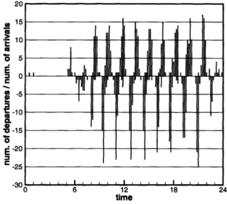
result is lower ticket costs and/or increased frequency of service for passengers. In hub-and-spoke networks, airlines typically operate banked schedules, in which are a set of arriving flights occurring in a relatively short period of time, followed by a set of departing flights also occurring within a short period of time. The amount of time separating the flight arrivals and the flight departures is defined by the amount of time needed for passengers to transfer, that is, connect between arriving and departing flight legs. Figure 2-1 shows the departure and arrival operations of a major U.S. airline at a banked hub. In this operation, there are 11 easily identifiable banks. A positive bar corresponds to the number of arrivals in a time interval, while a negative bar corresponds to the number of departures.

'E a C' CL 20 15 10 5 -5 -10 -15 -20 -25 0 6 12 18 24 time

Figure 2-1: Departure and arrival activities at hub in a banked schedule

Banked schedules create departure and arrival peaks at the hub, with each peak planned to last about 45-60 minutes. Peaking has associated negative economic im-pacts. For example, in order to process passengers and baggage during peak opera-tions, staffing requirements at the gate, on the apron, at the ticket counter, and in baggage handling, as well as infrastructure requirements (that is, runway capacity, gate capacity, baggage handling equipment, etc.) are at a maximum. Between adja-cent banks, however, there are typically 60 to 90 minutes of quiet time. During this

period, staffing requirements are low and hence, labor, equipment and infrastructure are not fully utilized.

Banked operations, with their peak demands for infrastructure capacity, exacer-bate the effects of congestion and delays. When bad weather conditions reduce airport capacity, two pronounced effects result. First, schedule delays are incurred, thereby increasing airline operating costs due to the extra crew and fuel costs when aircraft are queued to arrive or depart. Second, passenger travel times are increased, sometimes significantly if flight delays result in passengers missing their flight connections.

Yet another disadvantage of banked operations is the resulting reduction in air-craft productivity. First, because inbound flights in a common bank arrive at the hub at about the same time, aircraft operating flight legs with shorter flying times must wait at spoke cities and depart later than aircraft operating flight legs with longer flying times. This waiting time is non-productive time for aircraft, and very expensive to the airlines. Second, aircraft (especially those arriving early in the bank) must sit on the ground well beyond the minimum time needed to turn the aircraft, that is, the minimum time needed to re-fuel, disembark and embark passengers, and service the aircraft. Moreover, because the arrival times of inbound flights in a bank are coordinated, the departure times at spoke cities might not be convenient to pas-sengers. Similarly, because the departure times of outbound flights are coordinated, the arrival times at spoke cities again might not be convenient to passengers.

2.2.3

Moving Toward De-Peaked Schedules

The airline industry in the U.S. has been negatively impacted since 2001 by terrorist attacks, overcapacity, soaring fuel costs, and stiff competition. As a result, airlines have been forced to look for new approaches and strategies to achieve profitability.

Banked operations at hubs are very expensive, requiring a surplus of labor, equip-ment and infrastructure. De-peaked operations at hubs (also referred to as continuous or rolling hubs) can continue to take advantage of the hub-and-spoke network struc-ture, but with less intensive operations at the hub and therefore less cost (Donoghue, 2002; McDonald, 2002). In de-peaked schedules, arrival and departure operations

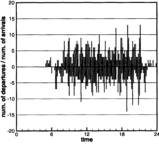
at the hub are smoothed, shaving the peaks and filling in the valleys of demand for resources. Flights are not coordinated in de-peaked operations to form connecting banks. Instead, the amount of time aircraft remain on the ground at the hub is not constrained by the need to provide passenger connections. Figure 2-2 shows the departure and arrival activities for the same airline shown in Figure 2-1 after the de-peaking of the same hub.

a, 'U .0 15 .4', I I E 5 C IA 0 0. 13 6 12 time 18 24

Figure 2-2: Departure and arrival activities at hub in a de-peaked schedule In summary, the benefits resulting from de-peaking hub operations include:

" Hub staffing can be reduced because the maximum number of arrivals and

departures occurring in a period of time for de-peaked operations is significantly smaller than that for peaked operations.

* Demands for infrastructure capacity, that is, airport runway and groundside capacity, gates, baggage handling equipment, etc., are similarly reduced in de-peaked operations.

" De-peaked schedules are more robust in the sense that airport capacity

reduc-tions caused by weather will have less of an impact than in the case of peaked operations with their high-levels of peak demand for capacity.

I II I I Ol . I . I ii I l

tL17 I

I

e In a de-peaked schedule, aircraft need not wait on the ground for connecting passengers. These reduced ground times for aircraft lead to increased aircraft utilization.

The major drawback of de-peaked operations is that the smoothed and spreaded-out arrivals and departures typically result in increased connection times for passen-gers. The effects of these increases on revenue are hard to quantify. Prior to the late 1990's, air tickets were mostly sold by travel agents using Global Distribution Systems (GDSs). Itineraries were displayed in increasing order of elapsed time, and the majority of bookings occurring in the first screen. Hence, increasing connection times, and thus, increasing elapsed travel time could displace an itinerary from be-ing displayed in the first screen and result in significant reductions in the number of bookings for that itinerary. The adverse effect of this, however, is mitigated by recent changes in distribution: the Internet has been gaining great popularity among trav-elers. In 2004, more than 22% of U.S. airline tickets were sold through the Internet

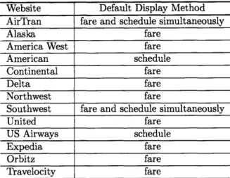
(Dorinson, 2004). In 2005, Alaska and its sister airline, Horizon, sold 34.6% of their tickets via the airlines' website and an additional 11% of the airlines' sales came via online travel sites (Gillie, 2006). Although travelers can choose to sort itineraries by schedule (departure time or elapsed time), the majority of air travel websites display search results by fare and researchers report that the fare display is most commonly used (Flint, 2002). GDSs also include fare display these days and fare display be-comes the most commonly used method by agencies (Flint, 2002). Table 2.1 shows an example of the default displays of major U.S. airlines and leading online air ticket retailers. 11 out of 13 websites offer fare as the default display (or fare and schedule display simultaneously).

2.2.4

De-Peaking in Practice

This section discusses examples of schedule de-peaking in the airline industry. While it is not intended to be a comprehensive and thorough coverage of this topic, it does suffice the purpose of demonstrating this industry trend and its impact.

Website Default Display Method AirTran fare and schedule simultaneously

Alaska fare

America West fare

American schedule

Continental fare

Delta fare

Northwest fare

Southwest fare and schedule simultaneously

United fare

US Airways schedule

Expedia fare

Orbitz fare

Travelocity fare

Table 2.1: Default display on the websites of major airlines and leading Internet air ticket retailers (obtained by visiting each website on March 6, 2006)

American Airlines de-peaked operations at its Chicago O'Hare (ORD) hub in April 2002. Flint (2002) reports that after de-peaking, the number of American Airlines flights remained the same as before, but arrivals and departures were more evenly spread throughout the day. In their de-peaked schedule, American Airlines restricted the number of arriving and departing flight legs per minute to no more than one.

Mean passenger connection times increased 10 minutes from 77 minutes to 87 minutes. Average aircraft turn times, however, reduced about 5 minutes, and by about 8 minutes at the spoke stations, resulting in less non-productive ground time for aircraft and, hence, increased aircraft utilization.

Benefits to American Airlines of de-peaking ORD include:

1. Fewer aircraft and gates were used to operate the same set of flight legs. It is

reported that 3 mainline jets, 2 RJs, and 4 gates were saved after de-peaking ORD (Flint, 2002). These saved aircraft can be put to use in an expanded flight schedule, complementing the cost-saving attributes of de-peaking with revenue-gain potential.

2. On time performance was improved despite higher aircraft utilization. After spending years at the bottom of the Department of Transportation (DOT) on-time performance scorecard, American rose to second place in the second

quarter of 2002. With reductions in air traffic congestion resulting from de-peaking, block times were reduced by more than one minute at ORD, worth $4.5-5 million per year (Ott, 2003).

3. Labor efficiency increased. Less people were needed to handle the same amount

of work, with each individual handling more flights per shift. The intensity of work per individual, however, does not increase because the workload is more evenly spread out through the day, unlike the peaked schedule in which periods of high levels of activity are followed by periods of little activity (Flint, 2002). 4. Revenues increased. American Airlines reported increased unit revenues

result-ing from a 1% improvement in the ratio of local (or, non-stop) to connectresult-ing traffic at ORD. Because flights are no longer coordinated to form banks at the hub, the departure and arrival times are set to convenient times for local markets, thereby attracting more non-stop passengers. Connecting revenues, however, declined as a result of longer connection times (Flint, 2002).

American airlines de-peaked its Dallas/Fort-Worth (DFW) hub in November, 2002. 9 mainline jets, 2 RJs, and 4 gates were saved (Flint, 2002). Because fewer gates are needed at DFW for their de-peaked schedule, American Airlines was able to move all mainline flights to Terminals A and C, both of which are on the same side of the airport. Previously, mainline flights operated in Terminals A, B, and C. In addition to the benefit to passengers of having all American Airlines flights on the same side of the airport, the airline estimates it will save at least $4.5 million annu-ally from this consolidation (SL, 2002). American Airlines subsequently de-peaked its Miami (MIA) hub in May 2004.

Besides American Airlines, Continental Airlines de-peaked its schedule at Newark (Ott, 2003); United Airlines de-peaked its hub in Chicago in 2004, its hub in Los Angeles in 2005, and is expected to de-peak throughout the system, beginning with San Francisco (SFO) in the first quarter of 2006 (UAL, 2006); and Delta Airlines de-peaked their Atlanta hub in January, 2005, where about 65 airplanes an hour arrive and depart throughout the day. Daily departures for Delta Airlines grew to

1,051 a day under the de-peaked schedule from 970 a day prior to de-peaking, and

the number of destinations served grew to 193 from 186. After de-peaking, average passenger connection times increased by about 3 minutes, up to 77 minutes from 74 minutes, and the amount of daily flying time per jet increased by about 8 percent, with the number of daily aircraft turns at each of the airline's gates increasing by up to 8.5 percent (Hirschman, 2004).

And, this de-peaking trend is not restricted to airlines the U.S.. Lufthansa Airlines de-peaked Frankfurt (FRA) in 2004, its biggest hub, as part of the effort to cut costs

by EUR 300 million in the next two years (Flottau, 2003).

2.3

Opportunities in a De-Peaked Hub-and-Spoke

Network

In a perfectly banked schedule, all inbound and outbound flights are scheduled to allow passengers to connect between any pair of arriving and departing flights in the same bank. Moreover, minor adjustments to flight arrival and departure times do not create, or eliminate, any connecting itineraries. In a de-peaked operation at a hub, however, minor adjustments to flight leg arrival and/or departure times can affect the set of connecting itineraries served through that hub. In fact, flight schedule re-timings can increase or decrease the supply of available seats in markets connecting at the hub. Figure 2-3 provides a schematic illustration of departure and arrival ac-tivities in a de-peaked hub-and-spoke network. We denote the minimum time needed for passengers to connect between flights at the hub as MinCT and the maximum connection time acceptable to passengers as MaxCT. Note that inbound flight a can-not connect to outbound flights b and c because the associated connection times are not within the allowable limits. Re-timing flight leg b to b', however, creates a feasible connection between flight legs a and b', as shown in Figure 2-4. This re-timing has the effect of adding seats to the market served by flight legs a and b'. At the same time, re-timing flight b to b', however, may cause some connecting itineraries using b as the

outbound flight to violate the maximum connection requirement, thereby decreasing

the number of seats offered in other markets. Similarly, re-timing flight c to c' creates

a feasible connection between flight legs a and c' and may cause some connecting

itineraries using c as the outbound flight to violate the minimum connection time

requirement, thereby decreasing the number of seats offered in other markets. The re-timing of flight legs can thus be considered a a powerful mechanism, one capable of dynamically adjusting the supply of seats to better match demands as revealed through the booking period.

a

MinC Mb MinCTu

6 c66cc

Figure 2-3: Original schedule Figure 2-4: Re-timing creates new

connecting itineraries

Flight re-timing has the added benefit that it can create more re-fleeting oppor-tunities, as illustrated in the examples presented in Figures 2-5 and 2-6. Figure 2-5 depicts the original schedule, in which an Airbus A319 operates flight leg a and then flight leg c, and an Airbus A320 operates flight leg b followed by flight leg d. Suppose that more capacity is desired on flight leg d and less capacity is needed on flight leg

c. The original schedule does not allow the same aircraft to operate both flight legs

b and c due to insufficient turn time between the arrival of b and the departure of c.

If b arrives earlier and c departs later, however, the A320 can operate b followed by c and the A319 can operate a followed by d, as depicted in Figure 2-6.

2.4

Modeling Architecture

In our dynamic scheduling approach, schedule re-optimization is performed for each departure date, thereby producing potentially different flight schedules, each of which is designed to capture the individual dynamics of passenger demand for that day. We

A319 A320 A319 20

A9 A329 A322 A319

c d c d

Figure 2-5: Original schedule Figure 2-6: New schedule

refer to the modified schedule for each day as the new schedule and to the schedule produced by the initial planning process as the original schedule. We assume that the original schedule is a daily schedule, that is, the same schedule is repeated each day.

Re-optimization points are points in time during the booking period when schedule

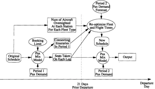
re-optimization, that is, flight leg re-timings and re-fleetings, is performed. A portrayal of our dynamic scheduling process is shown in Figure 2-7.

Departure Date 1 2 3 4 . Demand Profile

Re-opt Re-opt Re-opt Re-opt Point Point Point Point

Booking Starts

time

Figure 2-7: Dynamic scheduling process

For each day d included in the original schedule, we specify a few re-optimization points, with each re-optimization point earlier in the booking period of day d. Each schedule re-optimization results in a new schedule for a particular day, and it replaces the previous schedule, whether it is original or the result of re-optimization. At each re-optimization point for day d, three questions are answered, namely:

1. What are the current numbers of passenger bookings for each itinerary on day

d?

2. What are the forecasted future itinerary bookings from the re-optimization point to day d?

3. What is the set of optimal flight leg re-timings and re-fleetings for day d given the current and forecasted future itinerary bookings?

Any solution to the third question must satisfy the following constraints:

1. Flight legs can be re-scheduled only to a time close to that of the original

schedule. The set of allowable departure times for each flight leg defines that flight leg's feasible time window;

2. Allowable fleeting changes for a flight leg 1 are limited to fleet types in the same

family as that of the original fleet assignment to 1;

3. Service to passenger bookings made prior to the re-optimization point must be

guaranteed in the new schedule;

4. At the start of the day, the number of aircraft of each type available at each airport is equal to the number positioned at that airport at the end of the preceding day. At the end of the day in the new schedule, the number of aircraft of each fleet type at each airport location must be no less than the number in the original schedule. Because a daily schedule re-optimization model is used, this is equivalent to constraining the number of aircraft for each fleet overnighted at each airport to be no more than that in the original schedule.

Constraints (1) limit the magnitude of schedule changes to minimize the impact to passengers who booked their itineraries before the re-optimization point and the possibility to disrupt aircraft maintenance routing and crew pairing plans if they are developed prior the last re-optimization point. Constraints (2) ensure that crew assignments remain feasible after re-fleeting. Constraints (3) guarantee service to all previously booked passengers in the new schedule. The exact meaning of "service guarantee" is explained in Section 2.4.1. Constraints (4) ensure that aircraft are appropriately positioned at the end of the day so that the re-optimized schedule for the next day can be implemented.

2.4.1

Service Guarantee to Previously Booked Passengers

In order to minimize passenger inconvenience, passengers booked before the current re-optimization point are to be accommodated on itineraries with the same flight numbers, but potentially with a slight change in flight departure and arrival times. Re-fleeting does not change the timetable, therefore passengers wouldn't even notice such changes. However, re-timing affects the flight times and could potentially make the connection times for previously booked connecting itineraries shorter than the minimum required.

For nonstop passengers booked on flights prior to re-timing, the effect is a slight deviation of time for their flights. For connecting passengers booked prior to re-timing, we make sure that the re-timing decisions do not disrupt their itineraries, that is, their new connection times after re-timing are no less than the minimum connection time. For example, suppose a passenger booked the itinerary shown in Table 2.2. After re-optimization, the passenger will still be traveling on flight 254 and then connecting to flight 487 as before. The only thing that changes is the flight departure and arrival times. An example of the new itinerary is shown in Table 2.3. For the itinerary shown in Table 2.3, the connection time at the hub is 30 minutes, which is still greater than the 25-minute minimum connection time. Please note that the connection times of booked connecting itineraries are allowed to exceed the maximum connection time. When flight re-timing is limited to a small magnitude, which we envision to be ±15 minutes from the original timetable, the maximum possible increase in connection time is 30 minutes.

Flight Origin Departure Time Destination Arrival Time

254 BOS 9:00am HUB 12:00noon

487 HUB 12:45pm LAX 1:45pm

Table 2.2: Itinerary prior to re-timing

Flight Origin Departure Time Destination Arrival Time

254 BOS 9:10am HUB 12:10noon

487 HUB 12:40pm LAX 1:40pm

2.4.2

Frequency and Timing of Re-Optimization Points

While outlining the concept of dynamic scheduling in the previous section, we include several optimization points within the booking period. The question of when to re-optimize is, itself, an optimization problem. Because the objective of our research is to provide an estimate of the potential benefits of dynamic scheduling, we include only a single re-optimization point in the booking period. Even with this simplification, the question of when to perform this one-time schedule adjustment remains. The goal in selecting the re-optimization point is to balance flexibility to modify the schedule and

forecast quality. Forecast quality improves as the re-optimization point is moved later

in the booking period. Flexibility to modify the schedule, however, decreases as the re-optimization point is moved later in the booking period. This difficulty stems from passenger, crew and maintenance restrictions. Later in the booking period, in order to guarantee service to the large number of passengers who have already booked, the set of feasible re-optimization decisions are substantially constrained. With respect to crews and maintenance, if the re-optimization point occurs before the crew schedules and aircraft maintenance routings are constructed, crews and maintenance require-ments need not be considered in the re-optimization. If, however, the re-optimization point occurs after crew and maintenance plans have been generated, the new schedule must maintain feasibility of these plans or generate feasible alternatives.

2.4.3

Flow Charts

Using a single re-optimization point for each day d in the original schedule, for example 21 days prior to departure, the booking period is divided into two periods. We refer to the time period beginning at the start of the booking period and ending at the re-optimization point as Period 1; and the time period from the re-re-optimization point to day d as Period 2. Empirical results show that around 50% of the passengers have booked their itineraries 21 days prior to departure, providing valuable revealed demand information but leaving flexibility in the system.