Design and analysis of series elasticity in closed-loop actuator force control

(1)

Design and Analysis of Series Elasticity in Closed-loop

Actuator Force Control

by

David William Robinson

B.S., Mechanical Engineering

Brigham Young University

April 1994

S.M., Mechanical Engineering

Massachusetts Institute of Technology

June 1996

Submitted to the Department of Mechanical Engineering

in partial fulfillment of the requirements for the degree of

Doctor of Philosophy in Mechanical Engineering

at the

MASSACHUSETTS INSTITUTE OF TECHNOLOGY

June 2000

c

Massachusetts Institute of Technology 2000. All rights reserved.

Author . . . .

Department of Mechanical Engineering

May 11, 2000

Certified by . . . .

Gill A. Pratt

Associate Professor of Electrical Engineering and Computer Science

Thesis Supervisor

Certified by . . . .

David Trumper

Associate Professor of Mechanical Engineering

Thesis Committee Chair

Accepted by . . . .

Ain A. Sonin

Chairman, Department Committee on Graduate Students

(2)

Design and Analysis of Series Elasticity in Closed-loop

Actuator Force Control

by

David William Robinson

Submitted to the Department of Mechanical Engineering on May 11, 2000, in partial fulfillment of the

requirements for the degree of

Doctor of Philosophy in Mechanical Engineering

Abstract

Series elastic actuators have a spring intentionally placed at the actuator output. Measuring the spring strain gives an accurate measurement for closed-loop actuator force control. The low spring stiffness allows for high control gain while maintaining actuator stability. This gives series elastic actuators many desirable properties including high bandwidth at moderate force amplitudes, low output impedance, large dynamic range, internal error rejection and tolerance to shock loading. However, as a consequence of the elasticity, the large force bandwidth capabilities of the actuator are reduced when operating at power saturation limits.

Series elasticity is examined with three models. First, it is generalized by using a minimal actuator model. This mathematical model consists of an ideal velocity source actuator, linear spring and proportional controller. Series elasticity is then demonstrated in two case studies of physical actuator systems. The first is a linear hydraulic piston with a servo valve and the second is an electric motor with a geared linear transmission. Both case studies have a linear spring and low complexity control systems. The case studies are analyzed mathematically and verified with physical hardware. A series elastic actuator under simple closed-loop control is physically equivalent to a second order system. This means that an equivalent mass defined by the control system and physical parameters, is effectively in series with the physical spring connected to the actuator load. Non-dimensional analysis of the dynamics clarifies important parametric relationships into a few key dimensionless groups and aids understanding when trying to scale the actuators. The physical equivalent abstractions and non-dimensional dynamic equations help in the development of guidelines for choosing a proper spring stiffness given required force, speed and power requirements for the actuator.

Thesis Supervisor: Gill A. Pratt

(3)

(4)

Acknowledgments

MIT has given me an incredible education the last four years. It has stretched me academically and personally. I am very grateful to the people that have been with me to share this whole experience. I want to thank my advisor Professor Gill Pratt for his advice, guidance, help, time, and enthu-siasm. I appreciate all that I have learned from him as an advisor, teacher, mentor and especially as a friend.

I also want to thank the other members of my doctoral thesis committee: Professor David Trumper, Professor Haruhiko Asada, and Dr. J. Kenneth Salisbury. They have all made significant contributions to this thesis. Their direction and encouragement as a group and as individuals has been tremendous.

The Leglab is a great place to work because of the people. Dan Paluska, Ben Krupp, Jerry Pratt, Chris Morse, Andreas Hofmann, Greg Huang, Robert Ringrose, Mike Wessler, Allen Parseghian, Hugh Herr, Bruce Deffenbaugh, Olaf Bleck, Ari Wilkenfeld, Terri Iuzzolino, Joanna Bryson, Jianjuen Hu, Chee-Meng Chew, and Peter Dilworth have been great friends and colleagues. They have filled this experience with wonderful camaraderie in both work and fun.

I especially appreciate my good friends Brandon Rohrer, Sean Warnick, and Rick Nelson with whom I have shared the MIT engineering Ph.D. road. The time I spent working and in counsel with these men has been choice. They have each been marvelous examples to me in the ways that they balance family, service, work, school, and fun.

I thank my parents, brothers, sisters, and their families for their constant support, encourage-ment, and words of confidence. Mom and Dad are the ones who made it possible to start this journey and the whole family have always been there to see me through.

I particularly appreciate the support of my two daughters. Hannah’s smiles, hugs and clever wit have kept me going. MaryAnn’s recent arrival gave me the desire and motivation finish up quickly. They have both helped me to keep life in its proper perspective.

Finally, I give deep appreciation to my eternal companion Sarah. Our experience together has been full to overflowing. I am thankful for her faith, consistency, gentleness, kindness, and love. When you are with Sarah, how can your experience be anything but great! 143, always.

This research was supported in part by the Defense Advanced Research Projects Agency under contract number N39998-00-C-0656 and the National Science Foundation under contract numbers IBN-9873478 and IIS-9733740.

(5)

List of Figures

1-1 Series elastic actuator. The closed-loop actuator is topologically identical to any motion actuator with a load sensor and closed-loop feedback controller. The major difference is that the sensor is very compliant. Low spring stiffness removes gain from the power domain and and thereby allows for increased controller gain in the signal domain while still maintaining desired stability margins. . . 20 1-2 CAD models of the hydro-elastic actuator (left) and EM series elastic actuator (right)

developed and analyized in this thesis. Both actuators have a force output range on the order of 400–600 lbs. The power output for the hydro-elastic actuator is 1.5 kW and 430 W for the EM actuator. The minimum resolvable force of both actuators is approximately 1 lb due to the noise floor in the sensor. This gives the actuators a dynamic range of the order 500:1. . . 21 1-3 real Experimental bandwidth of the two prototype actuators. The hydro-elastic

actuator is on the left and the EM actuator is on the right. The magnitude of oscillation for the actuators is 40 lbs. The bandwidth of both actuators is in the range of 30-35 Hz. . . 22 1-4 real Experimental large force bandwidth. The actuators ability to sinusoidally

oscillate at the maximum force, Fsat, at steady state is limited in frequency due to

the spring compliance and motor saturation in force and velocity. The frequency at which that maximum force capabilities of the actuator begin to fall off is defined as

ωo. ωo= 25 and 8 Hz for the hydraulic and EM prototype actuators respectively. . 23

1-5 sim The EM actuator’s output impedance as a function of load motion input fre-quency under PD control. The plot comes from the dynamic equation derived in Chapter 5. The figure has been normalized in frequency by ωo and in magnitude by

the stiffness ks of the physical spring. At low frequency the impedance is small. The

impedance increases with increased frequency in the limit is equal to ks, the physical

spring stiffness. . . 24 1-6 Physical equivalent of output impedance. As xl drives at different frequencies, the

impedance of the actuator changes. At low frequency, the impedance looks like an equivalent mass, meq. At high frequencies, the impedance looks like the physical

elasticity of the spring in the actuator. Even though damping is not shown it is assumed present to limit uncontrolled oscillations at the natural frequency. . . 24 1-7 Series elastic actuator connected to an inertial load. Ideally the actuator is a perfect

force source (left). However, when moving and inertial load, the actuator has its physical equivalent impedance. Typically, meq is very small in comparison to the

load mass, ml. Nevertheless, understanding the relative magnitude of meq is important. 25

1-8 real Hydro-elastic actuator forces on an inertial load. The inertial load mass and the actuator equivalent mass are 18 kg and 20 kg respectively. Since the two are so close, at low frequency the actuator displays a significant non unity magnitude under PI control. The response magnitude rises as frequency increases and then drops at the closed-loop bandwidth of the actuator. . . 25

(8)

2-1 P3. A commercial walking robot built by Honda Research and Development. It uses

a combination of passive compliance in both its actuators and feet as well as active force control at the ankles. Reprinted with permission of Honda Motor Co., LTD. . . 31 2-2 Series Elastic Actuator. A spring is intentionally placed in series with an

eletro-magnetic motor, transmission and actuator output. The spring deflection is controlled thus inferring force control. . . 38 2-3 COG is a humanoid robot with upper torso, arms and head. There are series elastic

actuators for each of the six degrees of freedom in each arm. Here COG is turning a crank using a dynamic oscillating controller [76]. . . 39 2-4 Spring Flamingo is a planar bipedal walking robot. It uses series elastic actuators to

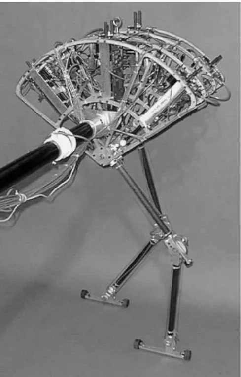
actuate its six joints. Its top walking speed is 1.25 m/s [50]. . . 39 2-5 Corndog is a planar running robot representing half of large dog. It uses the

electro-mechanical series elastic actuators developed as part of this thesis to actuate its four joints [34]. . . 40 2-6 M2 is a 3D bipedal walking robot. It has 12 degrees of freedom: 3 at each hip, 1 at

each knee and 2 at each ankle. The goal of M2 is to extend work done on Spring Flamingo to 3 dimensions. . . 40 2-7 Sarcos Dextrous Arm. It is a hydraulic force controlled teleoperated manipulator

that has been used for many applications including production assembly, undersea manipulation and hazardous material handling. The manipulator actuators have ac-cumulators on either side of the hydraulic fluid chambers. This gives the actuators intrinsic compliance. Reprinted by permission of Sarcos. . . 41 3-1 Minimal model for a series elastic actuators. There are four parts to a series elastic

actuator: elasticity, control system, motor, and system inputs. The compliance is a simple linear spring with a stiffness of ks. The force in the spring, fl, is equal

to the spring deflection times the stiffness. The control system consists of a simple proportional controller with gain K. The motor is modeled as a high impedance velocity source. The position output of the motor, xm, is the time integral of the

motor velocity. The system inputs or boundary conditions are the desired force, fd

and the load position, xl. . . 44

3-2 Graphical representation of the minimal motor model. The minimal motor model is a high impedance velocity source. It neglects inertia and has an instantaneous limit of force and velocity. It represents idealized models of both a hydraulic piston as well as an EM motor with a transmission. . . 45 3-3 General motor saturation model. All motors have limits to the instantaneous force

and velocity output capabilities. The line connecting the maximum load force, Fsat,

and the maximum actuator velocity, vsat, defines the envelope in which the motor can

operate. The slope of the saturation line is Ksat=_Fvsat

sat. . . 46

3-4 Minimal model and block diagram for a series elastic actuator. The figure on top is a time domain graphical representation of the the minimal series elastic actuator. The bottom figure shows a block diagram representation of the actuator. . . 47 3-5 Fixed load model and block diagram – case 1. (Top) A fixed load constraint defines

the closed-loop bandwidth of the system by isolating the relationship between desired force and load force. (Bottom) A block diagram of case 1 shows that the model is a simple first order system. . . 50 3-6 Zero order model for moving the gain from the power domain to the signal domain. A

series elastic actuator removes gain from the stiffness of the spring. The control system can then increase control gain while maintaining actuator stability. The stiffness of the spring is not a limiting factor in the closed-loop stability of the actuator. . . . . 51 3-7 Zero order model for reducing sensitivity to internal position noise. With sensor

stiffness gain and increased control system gain, internal position noise due to the transmission are greatly reduced. The provides for a very clean force output from the actuator. . . 52

(9)

3-8 Large force equals large elastic deformation. In order to create a large force, there must be a large elastic deformation. This requires the motor must move. In order to oscillate at high force amplitude, the motor must move very quickly. . . 53 3-9 sim_{Small force and large force bandwidth. The small force closed-loop bandwith}

is unaffected by the large force saturation constraints. However, as the magnitude of oscillation increases, the motor saturation dominates the large force output capa-bilities of the actuator. The more compliant the spring, the smaller the large force bandwidth. This is the key engineering tradeoff for series elastic actuators. . . 55 3-10 Forced load motion model and equivalent block diagram. (Top) The desired force is

fixed constant, Fd= Fo, and the load motion is defined externally. The relationship

between load motion and output force is defined as the output impedance. (Bottom) The block diagram shows that the feedback system and actuator dynamics are in the feedback loop. . . 56 3-11 Equivalent impedance for the general series elastic actuator. The active impedance

of the actuator can be thought of as an equivalent damper in series with the physical spring. At low driving frequencies, the actuator appears to be a damper. At high frequencies, the impedance is the stiffness of the spring. . . 57 3-12 General series elastic actuator with load mass moving in free space. In this particular

case, the load motion, xl, is explicitly defined as a function of the loads mass, ml, and

the force in the spring, Fl. . . 59

3-13 Equivalent model of the general series elastic actuator with load mass. The desired force is seen through a damper before the spring. A simple proportional controller does not make the actuator a force device. . . 60 3-14 sim General closed-loop forward transfer function (left) and output impedance (right).

These figures are normalized to the saturation frequency ωo and have κ = 3. . . . . 62

3-15 sim General large force saturation bandwidth. The ability of an actuator to output its full steady state force level is compromised by the introduction of a very compliant spring. ωo is the break frequency and is defined by the open loop dynamics of the

actuator. The large force bandwidth is typically less than the controlled bandwidth of the actuator. Even though the actuator cannot achieve full force output at high frequency, it can and does operate above ωo. . . 63

3-16 sim General force bandwidth profile with load inertia moving in free space. The variables in the figure are κ = 2 and L = 0.2. Any finite load inertia causes the system to have damper like qualities at low frequency as well as the bandwidth reduction at higher frequencies. As L→ 0, the system behaves as if it has a fixed load end. . . . 64 4-1 Prototype Actuator CAD model. A 20MPa pressure source is connected to a MOOG

series 30 flow control servo valve (not shown) that directs flow to the two chambers of the hydraulic cylinder. The piston is coupled to the output through four die compression springs. The spring compression is measured with a linear potentiometer which implies force. A closed-loop controller actively moves the piston to maintain a desired spring deflection. . . 66 4-2 Hydro-elastic actuator model. The servo valve directs fluid flow into the hydraulic

cylinder which moves the piston and thus compresses the elastic element. The strain in the spring is measured and used in a proportional-integral feedback control system. 66 4-3 Power domain model for the hydro-elastic actuator. The force output of the actuator

is determined by the compression of the spring. There are two inputs to the power domain. Q is the fluid flow from the servo valve and is a function of the input current

i. xl is a motion input from the environment. . . 67

4-4 simThe power saturation profile for a hydraulic servo valve is a square root relation-ship between flow and pressure. In order to understand the effects of saturation on the actuator through linear analysis, a linear saturation relationship is assumed. The linear profile is a worse case than the square root saturation. . . 70

(10)

4-5 sim_{This is a bode plot of the dimensionless closed loop system scaled to ω}_o_{. Values} for the plot were calculated from real parameters on the device: ωo= 152 rad/sec (25

Hz), κ = 2, I = 0.3 and V = 4.4. . . . 72 4-6 sim_{The impedance of the actuator at low frequency is zero and is k}_s _{at high}

fre-quency. The plot represents equation 5.14. It uses values ωo = 152 rad/sec (25 Hz),

κ = 2, I = 0.3 and V = 4.4 which were calculated from the prototype actuator. . . . 74

4-7 Rough characterization of hydro-elastic impedance. As shown in the simulation, the impedance at low frequencies is equivalent to a mass and is equal to the spring constant of the sensor at high frequencies. . . 75 4-8 Hydro-elastic actuator model with load inertia moving in free space. Unlike the

previous model where xlis a system input defined by the environment, in this model

the load inertia defines the motion of xlas a function of the force in the spring. The

load mass is part of the power domain and stores and releases kinetic energy as it moves. . . 76 4-9 Control abstraction for the hydro-elastic actuator pushing on an inertial load. Ideally,

the actuator produces the desired force directly on the load. However, the dynamics of the actuator turn out to be an equivalent mass and spring. The equivalent mass is defined by the control system and power domain characteristics. The spring is the actual physical spring in the actuator. . . 78 4-10 Prototype hydro-elastic actuator. The actuator has a piston with 0.2in2_{area in one}

direction and 0.15in2_{in the other. The piston pushes on precompressed die}

compres-sion springs. Spring deflection is measured with a linear potentiometer. Although not shown, fluid is directed into the piston via a servo valve with a 3000psi pressure source. . . 79 4-11 real Open-loop response for the servo, piston, spring and sensor. The solid line

represents the mathematical model and the dashed line is experimental data. The simulation model uses a full third order servo valve. The model captures all important features except the light damping on 800 Hz resonance of the real servo valve. . . . 81 4-12 real Closed loop response for the hydro-elastic actuator under PI control. The solid

line represents the mathematical model and the dashed line is experimental data. As in figure 4-11, the simulation model uses a full third order servo valve. The two models match very well in both magnitude and phase for the useful frequency range. . . 82 4-13 real PI control step response without and with servo valve dither. The integrator

in the controller keeps working on the errors in the system. Given that there is a small amount of stiction on the piston-cylinder interface, the integrator keeps hunting around the desired force. I add a small amount of dither on the to the servo valve and the hunting behavior disappears. Regardless of the dither, notice the fast response time of the actuator. The rise time is≈10 msec and the system is settled in 50 msec. 83 4-14 real Large force saturation for the hydro-elastic actuator. This is the response of

the actuator when it is oscillating at its maximum force for different frequencies. The large force performance begins to drop off near the predicted saturation point of 25 Hz. After the response starts to die off, the first order bandwidth limitations of the servo valve begin to come into effect. This effect is not accounted for in the simulation. Therefore, there is a difference in the experimental and simulated responses at frequencies above the saturation point. . . 84 4-15 Risky testing the elastic actuator. The author is suspended under the

hydro-elastic actuator. The actuator is supporting the load by a commanded force 1 lb above the downward force of gravity (∼ 250lbs). The author is holding a 2lb weight which drops the actuator. Releasing the weight causes the actuator to rise. The minimum resolvable force is 1 lb and is due to the noise floor of the sensor. . . 85 4-16 The hydro-elastic actuator rigidly connected to a hanging mass. The mass is 18kg.

By commanding desired force on the mass oscillating and different frequencies, the effect of the load mass can be verified. . . 85

(11)

4-17 real Actuator force output with an inertial load. The inertial load mass and and the actuator equivalent mass are 18 kg and 20 kg respectively. Since the two are so close, at low frequency the actuator displays a significant non unity magnitude under PI control as expected. The response magnitude rises as frequency increases and then drops at the closed-loop bandwidth of the actuator. Proportional control shows that the damper characteristics are significant for this actuator and inertial load combination. Using a proportional controller dramatically decreases low frequency force magnitude far beyond that of the PI controller. . . 86 4-18 real Results of drop testing an 18kg (40lb) mass attached to the actuator. At time

t =−0.2, the actuator is pulling the mass with an upwards force (force up is defined

negative). At about t≈ −0.15, the mass is released to drop. Even though the desired force of the actuator is set to zero, the impedance is not perfect and keeps pulling upwards with a 20lb force. At t = 0, the mass hits the end stop and the force spikes. The mass actually bounces a few times but the peak impact power is just after t = 0. 87 4-19 Model of the load mass during the drop test. Ideally, the load mass only feels the

force of gravity, F = mlg, since the actuator is set to output zero force (left). However

the actuator still has impedance. The gravity pull only affects the load mass. The equivalent mass of the actuator does not feel the gravity. Therefore, in order for the load to drop, the gravity force on the load must be distributed between the two masses, one real, one apparent (right). In the drop test case, the meq ≈ ml = 20kg

and the gravity force is distributed equally between the two inertias. . . 88 4-20 real Close-up of drop test impact forces. This shows the first impact of the load

mass. The impulse or change in momentum of the mass, J , is the area under the force curve. A numerical integration shows that J = 12kg· m_s. . . . 88 4-21 real Impact power. The top figure shows the force in the spring on the first impact.

By taking the area under the force curve, we can calculate the impulse, J , of the impact. J≈ 12kg ˙m/s. The middle figure shows the energy stored in the spring. It is

E = 1₂Fl2

ks. Finally, the impact power is estimated in the bottom figure by looking at

the rate of energy change P =∆E

∆t. The series elasticity spreads the impact time out

so that the required power is well within the actuator’s output power capabilities. . 90 5-1 The prototype actuator has a brushless DC motor rigidly connected to a ballscrew

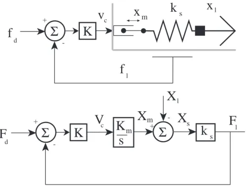
which drives the linear motion. The ballscrew nut is coupled to the output through four die compression springs. The spring compression is measured with a linear po-tentiometer. The actuator can output over 1350 N and move at 25 cm/second. . . . 92 5-2 Electro-magnetic series elastic actuator model. The motor mass has a driving force

and viscous friction. The controller drives the motor mass to compress the spring which gives the desired force output. . . 92 5-3 EM series elastic actuator power domain model. The motor mass has a driving force

and viscous friction. The Fl is the force output through the spring. . . 94

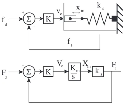
5-4 Electro-magnetic series elastic actuator model with a fixed load. This configuration helps to define the saturation limits of the actuator. . . 96 5-5 Velocity saturation model for the EM series elastic actuator. Simple velocity

satura-tion limits the ability of the amplifier to produce high forces. This model is slightly different than the force saturation model described in the previous chapters but has very similar results. Here Ksat=F_v_satsat. . . 98

5-6 simEM large force bandwidth due to force and velocity saturation. The motor mass spring resonance ωo defines the large force bandwidth of the actuator. The B group

(generalized damping) defines the shape of the profile around the saturation frequency. The three lines represent underdamped, critically damped, and overdamped frequency response. This plot only represents the large force capabilities of the actuator with the load fixed. . . 99

(12)

5-7 sim_{Closed-loop bode plot of the EM series elastic actuator with PD control. This} is a bode plot of the closed loop system with κ = 3 and ζc = 1. The zero from the

controller adds the apparent resonance near the controlled natural frequency. . . 101 5-8 simEM output impedance. The impedance of the actuator at small frequencies is

low and is equal to ks at high frequency. In this example κ = 4 and B = 0.1. For

low frequencies, the actuator has an equivalent mass characteristic. The equivalent mass is, meq = mκm. The higher the controller gain the lower the impedance. As Γ

increases there is an effective reduction in the impedance at the controlled natural frequency. . . 102 5-9 Rough characterization if EM impedance. As shown in the simulation, the impedance

at low frequencies is equivalent to a mass and is equal to the spring constant of the sensor at high frequencies. . . 103 5-10 sim Inverse parabolic relationship of the force error due to stiction force. As control

gain, Kp, increases non-linear friction forces are dramatically decreased. The two

curves represent the esimate of κ2. The solid line includes the +1 and the dashed line does not. In the physical actuator, Kp = 25. As can be seen, at that level of gain

there is very little difference between the two curves. . . 104 5-11 EM series elastic actuator model with load mass moving in free space. The load mass

defines the load motion xl . . . 105

5-12 sim Force on a load that is free to move. This plot shows that the actuator can output forces on a load mass even when it is free to move. . . 106 5-13 Control abstraction for the EM series elastic actuator. At frequencies below the

controlled bandwidth, the actuator can be considered a pure force source. Above the controlled bandwidth, the dynamics of the equivalent mass meq (equation 5.25) and

the spring come into play. . . 107 5-14 EM series elastic actuator used in testing. The actuator uses a brushless DC motor

with a direct connection to a 2mm lead ball screw. The ball nut drives the springs in series with the load. The springs are precompressed die compression springs. A linear potentiometer measures the deflection of the springs and uses that signal for feedback to the controller. . . 108 5-15 real Open loop bode plot for electro-magnetic series elastic actuator with fixed end

condition. This is a simple second order lumped mass spring system with a natural frequency of 7.5 Hz. The dynamic mass is the motor mass as seen through the transmission and the spring is the physical elasticity. . . 110 5-16 real Experimental maximum force saturation for the electro-magnetic series elastic

actuator with fixed end condition. The actuator can only generate the maximum output force up to the ωo, the mass-spring resonance frequency. . . 111

5-17 real Experimental closed-loop bandwidth for the electro-magnetic series elastic ac-tuator with fixed end condition. The -3dB point is at 35Hz. The zero in the closed-loop equation causes the apparent resonance. . . 111 5-18 Risky testing. The EM prototype actuator is suspended from the ceiling and loaded

with 300 lbs (me, seat and weights). The displacement of the spring is commanded so that it compensates for the gravity pull on the load mass. With small variations in the set point, the actuator moves the load up and down. . . 112 5-19 Fully loaded actuator demonstrating small force sensitivity. The actuator is fully

loaded with 300 lbs and has a force equal to gravity pull on the load mass. Finger force of approximately 1 lb can get the actuator to move up and down. This shows that the dynamic range of the actuator is 300:1. . . 113

(13)

List of Tables

2.1 Flow and effort for different power domains. Every power domain has variables that define the flow and effort of the medium. The product of these two variables is the power transferred in the system. . . 30 3.1 Comparison of sensor stiffness. The top load cell is a standard off the shelf component.

The bottom entry is the stiffness of the springs actually used in the prototype actua-tors of this thesis. The value shown is the one listed in the catalog. Experimentally, the springs were 12% more compliant. . . 56 4.1 Physical properties of Hydro-elastic prototype actuator. These properties are taken

from component literature and from experimental tests. . . 80 4.2 Important physical properties for force saturation. The point at which the

actua-tor begins to show signs of large force saturation is dependent upon these physical parameters. . . 82 5.1 Physical properties of EM prototype actuator. Some of the values are calculated from

motor literature and others are measured. . . 109 5.2 Itemized mass distribution for EM series elastic actuator. This actuator is used in

two dynamically stable robots described in Chapter 2. The table shows that over 50% of the mass is contained in the motor and magnet. In the design of series elastic actuators, it is important to keep the percentage power producing element mass high in comparison to the overall actuator mass. . . 113

(14)

(15)

Nomenclature

Force

Fd — Desired output force.

Fl — Measured output force in the spring.

Fe — Error between the desired and measured forces.

Fo — Constant desired output force.

Fsat — Maximum actuator output force at steady state.

Flmax — Maximum force amplitude of oscillation any a desired frequency.

Motion

xm — Position of the motor before the spring.

vm — Velocity of the motor before the spring.

xl — Position of the load.

vl — Velocity of the load.

xp — Position of the piston.

vp — Velocity of the piston.

xn — Position noise in the motor.

Vsat — Maximum actuator velocity.

Physical Parameters

ks — Actuator spring constant.

mm — Lumped motor mass.

ml — Load mass.

bm — Motor friction.

A — Piston Area.

τv — First order time constant of the servo valve.

meq — Physical equivalent actuator inertia.

beq — Physical equivalent actuator damping.

Frequency

ωo — Saturation frequency.

ωc — Controlled natural frequency.

ωl — Load mass (ml) spring (ks) resonant frequency.

Gain

K — Controller gain.

Km — General model motor gain.

Kv — Servo valve gain.

Ka — Motor amplifier gain.

Ki — Integral gain.

Kp — Proportional gain.

(16)

(17)

Chapter 1 Introduction

1.1 Thesis

Closed-loop control of series elasticity allows high-power density, high-impedance actuators to achieve low output impedance and good force sensitivity while maintaining good bandwidth. Intentional compliance in robot actuators is a deviation from traditional force control robot architecture. Nev-ertheless, series elastic actuators offer many advantages in force control tasks.

This thesis develops quantitative understanding of the effects, requirements and limitations for series elasticity in closed-loop actuator force control. The goals of the thesis are threefold:

1. Build a general framework for understanding series elastic actuators that is not dependent on a specific power domain.

2. Demonstrate and verify properties and limitations of series elastic actuators both mathemati-cally and with physical prototypes.

3. Give guidelines for choosing spring stiffness given force, speed and power requirements for the actuator.

General Framework

The ideas of series elasticity can be applied generally to high impedance actuation systems. A hydraulic piston and an electro-magnetic motor with a large reduction transmission are two examples. This thesis develops quantitative measures for understanding and describing series elastic actuators. Regardless of an actuator’s power domain, series elastic actuators exhibit good small force closed-loop bandwidth, reduced large force bandwidth and low output impedance.

Demonstration

This thesis demonstrates series elasticity both mathematically and physically with three models. First, a minimal actuator model generalizes the main ideas of series elasticity. This mathematical model consists of an ideal high-impedance velocity source motor, linear spring and proportional controller. Two case studies of physical actuator systems also demonstrate the principles of series elasticity. The first is a linear hydraulic piston with a servo valve and the second is an electric motor with a geared linear transmission. Both case studies have a linear spring and a low complexity control system, PI and PD respectively. The case studies include both mathematical analysis and physical hardware verification.

Choosing the Spring

The compliance of the spring in series elasticity is orders of magnitude less than traditional load sensors. Choosing a proper spring stiffness and designing an actuator that houses the elasticity

(18)

can prove challenging since the spring travel is so large. In this thesis, I explain the fundamental tradeoffs of spring stiffness in balancing the requirements for large force bandwidth and low output impedance. Through the use of non-dimensional models, a designer can also understand the effects of different spring stiffnesses in order to scale the actuator.

1.2 Motivation

The vast majority of commercial robot applications consist of tasks that control the position1_or

tra-jectory of each robot degree of freedom. Traditional robots can do this with great speed, endurance, precision and accuracy. Robots have been used in this commercial niche because repetitive tasks which require precision and accuracy are difficult and tedious for humans.

On the other hand, there are many tasks in which robot competence is inferior to that of biological counterparts. Despite extensive research, actions such as walking, running, swimming, catching, grasping and manipulation, considered easy to most able-bodied humans, are difficult for robots. These tasks all require interacting with the real world.

Since our world is kinematically and inertially constrainted, it is important for a robot to be able to sense and control the interaction forces between itself and the environment. This is typically referred to as Force Control.2 There are two aspects to successful force control. The first is to use an algorithm and sensory information to determine the desired robot joint torques in order to place the proper forces on the robot’s environment. The second aspect of successful force control is to generate accurate forces at the robot joints. This thesis deals with the second aspect of force control and specifically on the actuators that create the forces.

Present-day actuation technology is typically poor at generating and maintaining accurate forces. Using local closed-loop control of actuator forces can improve the quality of force output by reject-ing disturbances. Furthermore, it has also been shown that usreject-ing a compliant load sensor in a configuration called Series Elasticity, increases an actuator’s ability to generate accurate forces.

The focus of this thesis is to analyze and quantify the effects of load sensor compliance for closed-loop actuator force control. There are some unifying principles of series elasticity that can be captured in a general mathematical model. These general principles are further developed with specific models and physical prototypes for the hydraulic and electro-magnetic (EM) power domains. This introductory chapter defines and outlines the qualities of good force control actuators. It also describes the first implementations of Series Elastic Actuators as a deviation from traditional actuator design. Finally, it gives a summary of the thesis results and contributions.

1.2.1 Actuation and Force Control

Actuation is the process of converting some form of energy into mechanical force and motion. An actuator is the device or mechanism that accomplishes this energy conversion process. An electro-magnetic motor with a gear transmission and a hydraulic piston are two examples of such actuators. With few exceptions, standard robot actuation systems are poor at creating accurate forces in robot joints. The reasons for this inaccuracy include friction, stick-slip, breakaway forces on seals, backlash in transmissions, cogging in motors and reflected inertia through a transmission. All of these real phenomena induce force noise in the actuator. The effects of force noise are minimized when controlling the position or trajectory of the robot. The mass in both the robot and the actuators low-pass filter force noise on positional output. This is one reason why robots are so successful at trajectory control even in the face of force noise. However, for tasks requiring good force control, the force noise in the actuators can be problematic.

Good force-controlled actuators have several important measures: force bandwidth, mechani-cal output impedance, dynamic range, power density and force density. The first three measures are related to one another, and typically an improvement in one yields an improvement overall.

1_{The term position is the generalized position/orientation vector.} 2_{The term force denotes a generalized force/torque vector.}

(19)

An increase in power or force density usually means that the other three characteristics suffer in performance.

The force bandwidth is a measure of how quickly the actuator can generate commanded forces. Bandwidth is the highest frequency at which the actuator creates a near one-to-one output force to desired force.3 The bandwidth must be sufficient to transmit accurate forces through the robot structure. Most force control tasks only require a few hertz bandwidth as demonstrated by the low bandwidth of human muscle. However, improving the bandwidth of the actuator above the minimal operational level can only improve the overall capabilities of the robot.

Mechanical output impedance4is defined as the minimum amount of force an actuator outputs for a given load motion. In the simplest terms it can be thought of as the stiffness of the actuator output. Ideally, the impedance of a force controlled device is zero. Low impedance means that the actuator appears to the robot as a pure force source with negligible internal dynamics. An actuator with low impedance is sometimes referred to as being backdriveable.

Dynamic range is the maximum output force divided by the minimum resolvable output force

increment of the actuator. It gives a measure for how sensitive the actuator is to small forces with respect to its full force output capability. A large dynamic range is desirable because it permits the actuator to be used in a versatile way in both very sensitive activities and in large force situations. Humans have very good dynamic range.

Force density and power density are not necessarily operational characteristics. Nevertheless,

these qualities refer to an actuator’s ability to generate force or deliver power to the robot per unit mass and unit volume of the actuator. Having high force and power density means that a small package can output a lot of energy. Lightweight actuators prevent over-burdening the robot structure with excess mass and allow for quick, responsive robot performance.

Electric motors with gear reductions and hydraulics are two present-day actuator systems that have high force and power density and can also achieve moderate to high bandwidth. Unfortunately, neither system possesses low impedance or large dynamic range qualities required for good force control.

1.2.2 Series Elastic Actuators

The force output capabilities of a standard actuator such as an electric motor with gear reduction or a hydraulic piston can be dramatically improved by using a load sensor as feedback for a closed-loop control system. This technique has been used for many years on both actuator closed-loop force control and robot endpoint force control.

Standard load sensors are designed to be as stiff as possible for a given load. This allows the sensor to transmit power interactions with no internal storage of energy. Unfortunately, a stiff load cell in series with an already stiff actuator means that the open-loop gain of the actuator is very high. This in turn implies that to maintain actuator control stability, control gains must be kept low. Low control gains typically indicate poor overall closed loop performance. Low control gains, high impedance actuators and stiff sensors make for a system that cannot handle shock loads from the environment or filter out friction and other transmission non-linearities inherent in real systems.

To overcome these deficiencies, several investigators including Howard [29] and Pratt and Williamson [46, 75] experimented with a closed-loop control of an electro-magnetic motor and gear reduction in series with a compliant spring. Information about force in the spring is obtained by measuring the spring strain or deflection. Pratt and Williamson named this actuator configuration a Series Elastic

Actuator.

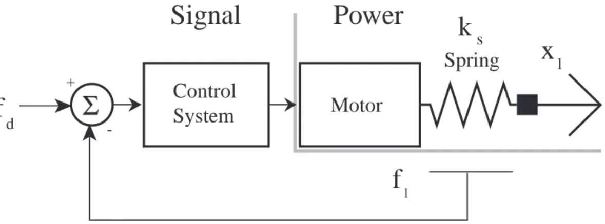
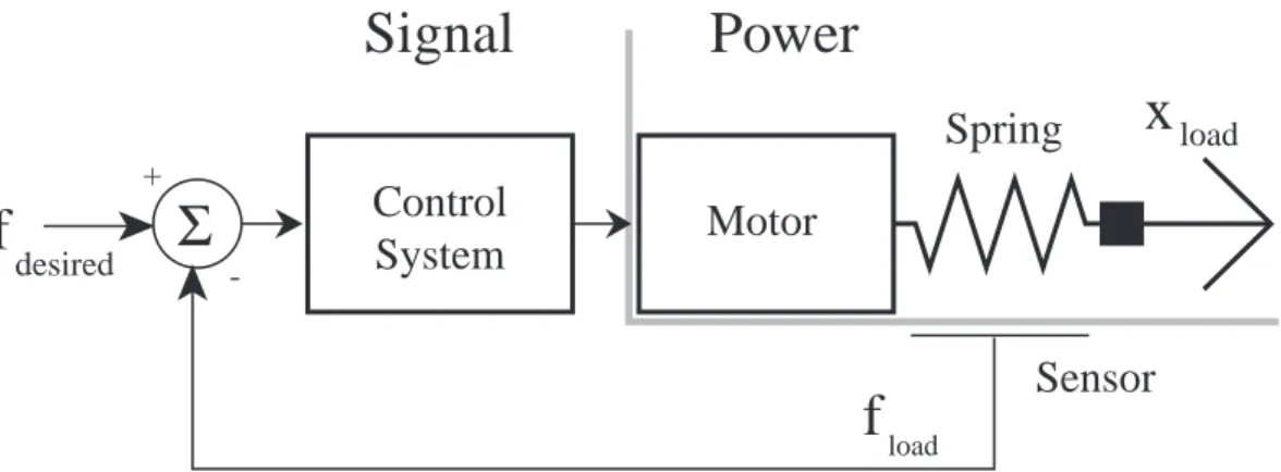
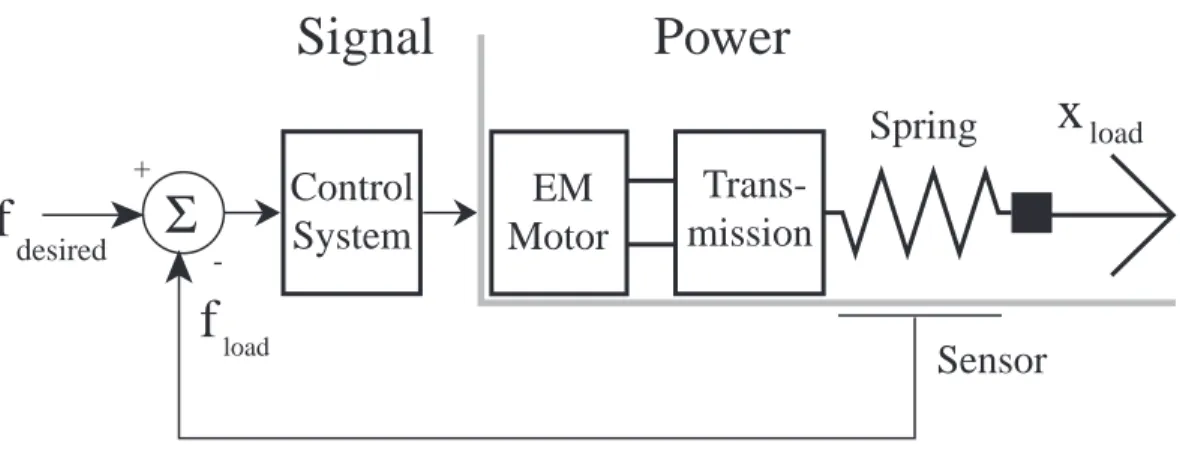
Figure 1-1 shows that series elastic actuators are topologically similar to any motion actuator with a load sensor and closed-loop control system. However, there are two significant differences resulting from the compliant element. First, there is increased energy storage in the spring that cannot be neglected. Second, integration of a compliant load-bearing sensor within a compact actuator can prove challenging. Nevertheless, compact designs have been successfully developed.

3_{A -3dB magnitude of output force to desired force is typically considered the bandwidth. -3dB is roughly 70%.} 4_{Throughout this thesis mechanical output impedance is referred to as impedance or output impedance.}

(20)

load

Control

System

Motor

Sensor

Spring

f

desired +

-Σ

Signal

Power

x

_load

Figure 1-1: Series elastic actuator. The closed-loop actuator is topologically identical to any motion actuator with a load sensor and closed-loop feedback controller. The major difference is that the sensor is very compliant. Low spring stiffness removes gain from the power domain and and thereby allows for increased controller gain in the signal domain while still maintaining desired stability margins.

The primary advantage of series elasticity is that the compliant load bearing sensor lowers the loop gain of the closed-loop system. The control gain can be proportionally increased to maintain the overall loop gain of the actuator at desired stability margins. This allows series elastic actuators to have low output impedance, be tolerant to shock loading and robust to changing loads. In addition, the increased controller gain greatly reduce the effects of internal stiction and other transmission non-linearities to give the actuators clean force output.

Many other research and commercial groups have recognized that purposeful compliance in ac-tuators can be beneficial for force control. Several of these ideas and implementations in both stand-alone actuators and complete robots are described in Chapter 2. For the most part, in the past, the advantages of compliance in actuators, including series elastic actuators, have been explained with intuitive reasoning and not with mathematical demonstration.

In this thesis, I build quantitative understanding for closed-loop control of series elasticity. I also give performance measures for the actuator. These measures include closed-loop bandwidth, large force bandwidth, output impedance and inertial loading effects. These performance measures can be used to help guide actuator design, especially in choosing the stiffness of the elasticity. A brief summary of thesis highlights are given next.

1.3 Highlights of thesis results

The series elastic actuator shown in figure 1-1 is representative of the general model and the two physical actuators built for this thesis. Using minimal control the actuators achieve good bandwidth, low output impedance and large dynamic range.

As a brief summary of the thesis, I focus on results from the physical actuators. I first describe some of their general capabilities such as maximum force, power output and dynamic range. Then, by looking at specific cases of the actuators in operation, we can discuss other actuator measures: bandwidth, output impedance and the effects of an inertial load.

1.3.1 Actuators

Figure 1-2 shows CAD pictures of the two actuators designed, built and tested in this thesis. The left picture is of the hydro-elastic actuator and the right picture is the EM series elastic actuator. Both actuators have similar maximum force levels (400–600 lbs). The hydro-elastic actuator has

(21)

Figure 1-2: CAD models of the hydro-elastic actuator (left) and EM series elastic actuator (right) developed and analyized in this thesis. Both actuators have a force output range on the order of 400–600 lbs. The power output for the hydro-elastic actuator is 1.5 kW and 430 W for the EM actuator. The minimum resolvable force of both actuators is approximately 1 lb due to the noise floor in the sensor. This gives the actuators a dynamic range of the order 500:1.

significantly higher power capabilities (1.5kW) compared with the EM actuator (430 W). The power density is also very high.

Without series elasticity, both actuators have high output impedance and are poor at open-loop force control. However, with series elasticity, the actuators are very force sensitive and can achieve high bandwidth at moderate force amplitudes. The closed-loop actuators have low output impedance. The lowest resolvable force, which is limited by the noise floor of the sensor, is approx-imately one pound, giving a dynamic range on the order of 500:1. The low output impedance also helps to significanly decouple the actuator dynamics from that of an inertial load.

1.3.2 Bandwidth

Bandwidth is a measure of how well the actuator can output a load force or force in the spring, Fl,

given a desired output force, Fd. The closed-loop bandwidth, or the relationship between Fl and

Fd, changes with frequency and can be written as a transfer function of the form

Gcl(s) =

Fl(s)

Fd(s)

.

The proposed bandwidth is measured with the load position of the actuator output held constant. This is analogous to when the actuator is in rigid contact with an unyielding environment or if the actuator is connected to an infinite load inertia.

I examine two cases of bandwidth. The first is the small force closed-loop bandwidth and the second is the large force bandwidth when the actuator is operating at full force and velocity saturation limits.

Small force bandwidth

The fundamental limits in small force bandwidth for series elastic actuators are independent of the spring stiffness that senses the force. The control system gain and the spring stiffness gain each contribute to the loop gain of the closed-loop system. With a lower spring stiffness the controller gain can be increased a proportional amount to bring the loop gain to the desired phase and gain stability margins.

(22)

100 101 102 -30 -20 -10 0 10 Fl /Fd (dB) Experimental Simulation 100 101 102 -200 -150 -100 -50 0 Phase (degrees) f (Hz) Experimental Simulation 100 101 102 -30 -20 -10 0 10 Experimental Simulation 100 101 102 -200 -150 -100 -50 0 f (Hz)

Phase (degree) Experimental_Simulation

Fl

/F

(dB)

d

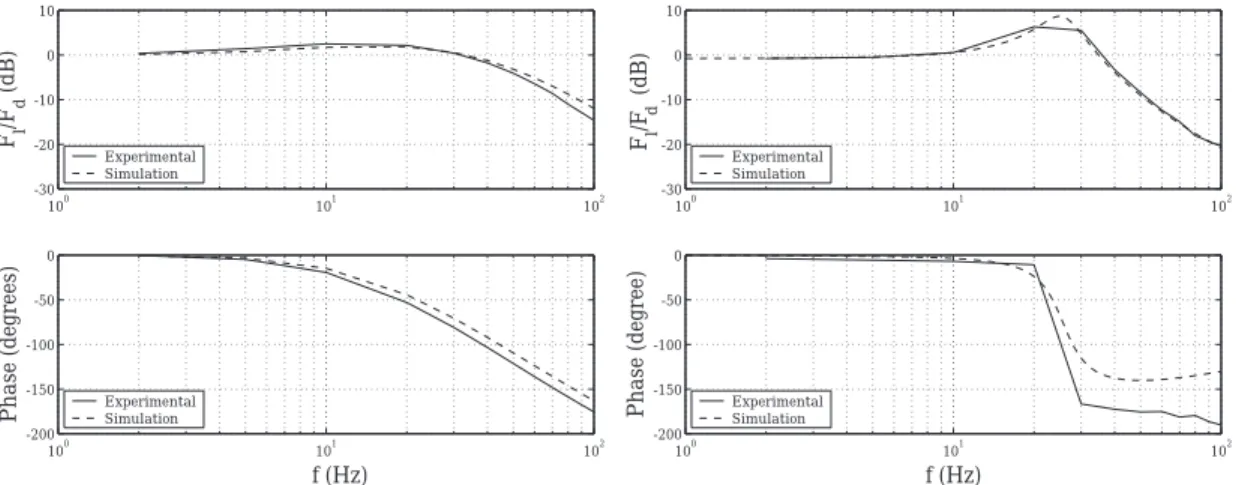
Figure 1-3: real _{Experimental bandwidth of the two prototype actuators. The hydro-elastic} actuator is on the left and the EM actuator is on the right. The magnitude of oscillation for the actuators is 40 lbs. The bandwidth of both actuators is in the range of 30-35 Hz.

Assuming that the actuator is operating in a non-saturated state, we can measure the bandwidth. Figure 1-3 shows the closed-loop bode plots for both the hydro-elastic actuator (left) and the EM series elastic actuator (right). The force amplitude of oscillation for the test is 40 lbs. Each actuator has a bandwidth in the range of 30-35 Hz.

Large force bandwidth

Elasticity requires that there is a large elastic deformation in order to achieve a large force. High force amplitude oscillations require that the motor must move very fast. However, all motors have force and velocity saturation limits. Closed-loop analysis of the series elastic actuator does not apply when the actuator is operating at saturation levels. Motor saturation places a limit on the large force bandwidth. Large force bandwidth is defined as the frequency range over which the actuator can sinusoidally oscillate at a force amplitude equivalent to the maximum output force Fsat at steady

state.

The large force bandwidth or saturation bandwidth, referred to as ωo, is typically less than the

closed-loop bandwidth when using a series elastic force sensor. The actuator can still produce force above ωobut the maximum force capability decreases with increased frequency.

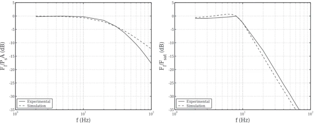
Figure 1-4 shows the large force bandwidth for the hydro-elastic actuator on the left and the EM series elastic actuator on the right. As with the small force closed-loop bandwidth, the large force bandwidth is tested with the load end of the actuator fixed. ωo = 25 and 8 Hz for the hydraulic

and EM actuators respectively. It is important to note there that that the actuators are oscillating sinusoidally at full saturation force (over 400 lbs)!

The large force bandwidth, ωo, for the hydro-elastic actuator is a function of the spring stiffness,

piston area, maximum flow rate of the valve and the supply pressure. For the EM actuator, the large force bandwidth is defined at the natural frequency of spring and reflected motor inertia. Understanding and carefully defining an appropriate ωofor a series elastic actuator is important in

(23)

100 101 102 -35 -30 -25 -20 -15 -10 -5 0 5 f (Hz) F l /P s A (dB) Experimental Simulation 100 101 102 -35 -30 -25 -20 -15 -10 -5 0 5 f (Hz) F l /F sat (dB) Experimental Simulation

Figure 1-4: real Experimental large force bandwidth. The actuators ability to sinusoidally oscil-late at the maximum force, Fsat, at steady state is limited in frequency due to the spring compliance

and motor saturation in force and velocity. The frequency at which that maximum force capabilities of the actuator begin to fall off is defined as ωo. ωo = 25 and 8 Hz for the hydraulic and EM

prototype actuators respectively.

1.3.3 Output Impedance

As defined previously, output impedance is the amount of force at an actuator output given a moving load position. This can be written as a transfer function in the form

Zcl(s) =

Fl(s)

xl(s)

.

Ideally the actuator is a pure force source and has zero output impedance. If this were the case, the dynamics of the actuator would be completely decoupled from that of the load motion. However, since the actuator is a real system, it has some output impedance.

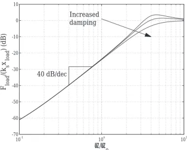
Figure 1-5 shows the calculated the EM actuator’s output impedance as a function of load motion input frequency under PD control. The plot comes from the dynamic equations derived in the thesis. The impedance of the hydro-elastic actuator under PI control is almost identical to that of figure 1-5 and is therefore not shown. The figure has been normalized in frequency by ωoand in magnitude by

the stiffness ksof the physical spring. The load motion is assumed to be a high-impedance position

source. At low frequency the impedance is small. The impedance increases with increased frequency in the limit is equal to ks, the physical spring stiffness.

The passive compliance in the spring and the active control system both contribute to the low impedance of the series elastic actuator.

The spring’s stiffness can be more than two orders of magnitude lower than a standard load sensor. Even without closed-loop control, the spring lowers the impedance. This effect is most noticeable at high frequencies.

The second effect is due to the active control system. With a decreased sensor stiffness, the control gain is increased. This effect is noticeable at low frequencies. Notice that the impedance is rising at 40 dB per decade which means that the output impedance has two zeros at the orgin in the dynamic equation. This implies that at low frequency

Fl= meqs2Xl.

(24)

10-1 100 101 -70 -60 -50 -40 -30 -20 -10 0 10 F load /(k s x load ) (dB) ω/ω o Increased damping 40 dB/dec

Figure 1-5: sim The EM actuator’s output impedance as a function of load motion input frequency under PD control. The plot comes from the dynamic equation derived in Chapter 5. The figure has been normalized in frequency by ωo and in magnitude by the stiffness ksof the physical spring.

At low frequency the impedance is small. The impedance increases with increased frequency in the limit is equal to ks, the physical spring stiffness.

actuator. To give a sense of the equivalent mass, I define it for the EM series elastic actuator

meq =

mm

K

where mm is the reflected motor inertia and K is the overall gain in the control system. In a

series elastic actuator, the control system gain, K, is very large. Therefore, the equivalent inertial impedance, meq, is small relative to the reflected motor mass, mm.

The output impedance is shown graphically in figure 1-6 as a physically equivalent mass in series with the spring driven by the load motion. Eventhough the impedance of the actuator is not zero, it is small.

k

m

_eq _s

x

load

Figure 1-6: Physical equivalent of output impedance. As xl drives at different frequencies, the

impedance of the actuator changes. At low frequency, the impedance looks like an equivalent mass,

meq. At high frequencies, the impedance looks like the physical elasticity of the spring in the

actuator. Even though damping is not shown it is assumed present to limit uncontrolled oscillations at the natural frequency.

(25)

m

_l

x

_l

x

_l

k

F

m

eq d s l

F

_d

Figure 1-7: Series elastic actuator connected to an inertial load. Ideally the actuator is a perfect force source (left). However, when moving and inertial load, the actuator has its physical equiv-alent impedance. Typically, meq is very small in comparison to the load mass, ml. Nevertheless,

understanding the relative magnitude of meq is important.

100 101 102 -25 -20 -15 -10 -5 0 5 F l /F d (dB) 100 101 102 -150 -100 -50 0 50 f (Hz) Phase(degrees) Experimental Simulation Experimental Simulation

Figure 1-8: real Hydro-elastic actuator forces on an inertial load. The inertial load mass and the actuator equivalent mass are 18 kg and 20 kg respectively. Since the two are so close, at low frequency the actuator displays a significant non unity magnitude under PI control. The response magnitude rises as frequency increases and then drops at the closed-loop bandwidth of the actuator.

1.3.4 Load Motion

Series elastic actuators are meant to be used in real-world robots that contact the environment. However, there are many times when such a robot is simply moving an inertial load in free space. In this case, the load motion is defined by the mass of the load, ml, and the force through the actuator.

Ideally, a series elastic actuator can be considered a pure force source within the controlled bandwidth independent of the load mass. However, as just explained, the impedance of the actuator is not perfectly zero. The actuator does have minimal dynamics that must be considered when looking at the force the actuator applies to a freely moving inertial load. Figure 1-7 graphically depicts the difference between the ideal force source (left) and with the impedance model (right).

When ml meq then the dynamics of the actuator are negligible to within the actuator

band-width and the actuator can be considered a force source. However, the closed-loop force transfer function changes at low frequency if the load inertia is close to or less than that of the impedance equivalent mass, meq. In the limit, if there were no load mass, the actuator has nothing to push on

and produces no force.

(26)

load. The inertial load and equivalent mass of the actuator are 18 kg and 20 kg respectively. At low frequency, the force on the load is a little less than half of the desired force. As force frequency increases, the response magnitude rises and then drops at the closed-loop bandwidth of the actuator. In summary, series elastic actuators have many desireable properties as force controllable ac-tuators. The high bandwidth, low impedance, shock tolerance, internal non-linear error rejection and large dynamic range are balanced with reduced large force bandwidth and reduced load force response. Understanding these tradeoffs is the key to successfully applying series elastic actuators in robot systems.

1.4 Thesis Contributions

The contributions of this thesis are:

1. A presentation of a minimal model for series elastic actuators that aids in understanding the fundamental principles of the actuators.

2. The design and construction of a linear hydro-elastic actuator that uses a linear piston and servo valve.

3. The design and construction of a modular electro-mechanical series elastic actuator that uses a brushless DC motor and linear transmission.

4. The development of linear models for both the hydro-elastic actuator and EM series elastic actuator.

5. The clarification between small and large force bandwidth and a discussion of bandwidth limits. 6. The development of intuitive physical equivalent models that represent actuator impedance. 7. The development of a linear model for the actuator connected to an inertial load moving in

free space.

8. The demonstration and explanation of impact tolerance in series elastic actuators.

9. The reformulation of the linear models into dimensionless terms that aids in understanding important relationships in actuator scaling.

10. The explanation of choosing spring stiffness for actuator design and development.

1.5 Thesis Contents

The thesis is organized as follows:

Chapter 1 gives a brief introduction to the background and motivation of the thesis. It also includes a summary of the thesis objectives and covers the key results from the research.

Chapter 2 presents detailed background material and related work covering general ideas of force

control, present-day actuator technology and actuators which use compliance.

Chapter 3 describes a minimal model of series elastic actuators. This model contains all of the

key characteristics of a compliant load sensor used in closed loop force control.

Chapter 4 applies results of chapter 3 to a case study for a hydraulic piston, a hydro-elastic

actuator. The theoretical model is compared with experimental results.

Chapter 5 applies results of chapter 3 to another case study of an electro-magnetic motor with a

gear reduction. The theoretical model is compared with experimental results.

(27)

1.6 Note on thesis data

This thesis includes data from both mathematical models and hardware. The figure captions indicate the source of the data. Simulated figures are marked sim and figures from hardware are marked real. real is also used when both simulated and real data are compared in the same figure. This notation method is adapted from Williamson [76].

(28)

(29)

Chapter 2 Background and Related Work

Robots are very successful at performing tasks that require movement in free space or known en-vironments under position control. Tasks such as spray painting vehicle exteriors, pick and place of IC chips, arc welding and spot welding fit very well into this paradigm. While many robotic applications that use position control have found their way into the commercial sector, robots that contact the surrounding environment and work within kinematic constraints have for the most part been limited to laboratory research. In fact, simple tasks such as driving a screw, turning a crank, assembling toys, and writing on a chalk board are extremely difficult for most robotic manipulators [5]. Instead of position control, these robots require force control. The robots themselves must be capable of accurately modulating and controlling actuator torques and forces.

This chapter explores the background of force control and force controllable actuators and pro-vides explanations of applicable previous work. Some explanations of different techniques and algo-rithms to achieve robot compliance are outlined. The bulk of the chapter discusses capabilities of different actuator systems and how each performs with respect to force control. Actuators with in-tentional compliance, specifically series elastic actuators, are also discussed with examples of related work in both the electro-magnetic and hydraulic domains.

2.1 Force Control

Force Control is the term used to describe the necessary interaction between a robot and an external

unknown environment. The robot must have the capability of sensing and controlling forces in addition to knowing where it is in its work space.

The necessity for force control deserves some discussion. Paynter gives a general explanation for maintaining proper causality when any two physical systems interact energetically [43]. The two systems’ interaction is defined at the interface by a set of orthogonal variables: flow and effort. In a mechanical system, flow is the velocity or motion and effort is the force. In any power domain (such as mechanical, hydraulic, electric, thermal, etc.) there are equivalent flow and effort variables (Table 2.1). The product of these two variables is the power transferred across the system interface. Interestingly, one physical system cannot independently control both the flow and the effort at the point of interface. A system may define and control one of these variables or a relation between the two variables, but not both.

This explanation of general physical system interaction has direct application for why force control is necessary when a robot interacts with an unknown environment. Most workpieces and environments with which a robot will interact are inertially and kinematically constrained. A pallet has mass. A door swings on a hinge. A wall and floor are vertical and horizontal barriers respectively. Given these constraints the environment often defines the flow interaction. This leaves the robot with only the option to modulate the effort. In other words, while the robot can push on and give energy to the environment, it cannot specify how the environment will respond. If the robot tries to control the position at a constrained interface, there exists a basic incompatibility between the two physical systems. Therefore, whenever a robot interacts with an environment or workpiece and is

(30)

Power Domain Effort Flow

Mechanical Force (N) Velocity (m/s) Hydraulic Pressure (Pa) Flow rate (m3/s)

Electric Voltage (V) Current (A)

Thermal Temperature (K) Entropy rate (J/Ks)

Table 2.1: Flow and effort for different power domains. Every power domain has variables that define the flow and effort of the medium. The product of these two variables is the power transferred in the system.

not simply moving around in free space, it must use force control. While it is still important for the robot to understand its own sense of position, it also needs some capability of being compliant in order to effectively match the given constraints. As defined in the introduction, the robot must have low impedance. This allows the causality of the robot-environment interface to maintain a proper relationship.

It is important to point out that all environments do have some compliance. While most con-straints have high stiffness, there are other environments which are very compliant such as sod or carpet. In fact some systems, like water, can exhibit variable compliance depending on the con-ditions. In these cases it may be necessary to control some linear combination of flow and effort. Nevertheless the robot must be capable of being compliant. It cannot be limited to high stiffness. Therefore, responsive force control is essential.

The following three subsections cover different techniques, ideas and algorithms that robot op-erators use in order to match compliance requirements with the environment. This includes passive methods as well as active control. The discussion also outlines some robotic applications where force control can be very useful.

2.1.1 Passive Compliance

A simple method to achieve pseudo force control and low robot output impedance is to have a robot use conventional position control but incorporate passive compliance. Passive compliance can be found in the robot structure, joints, and at the end effector. It differs from active force control in that passive compliance does not use force information for feedback to modulate the control algorithm. There are two major ideas behind passive compliance: low servo stiffness and passive end effectors. By introducing passive compliance into the joints, the loop gain for the position control loop is effectively softened. A similar effect can be achieved by increasing the compliance in the robot structure (links). With a combination of low servo stiffness and low structural rigidity, the robot may be able to successfully interact with a work piece or environment simply by using position control schemes. However, the risk of adding too much compliance to a robot is that the robot may be sloppy in its task execution and may fail in its overall goal [16].

Successful examples of passive compliance in robot joints are the bipedal walking robots built by Honda Research and Development called P2 and P3 (figure 2-1 shows two views of P3). P3 is slightly smaller than P2. Both robots use a compliant damping material as a coupling between the robot actuators and joints [17, 24]. The coupling protects the robot’s actuators from the shock loads in each step and decouples the reflected inertia through the large Harmonic drive gear reduction. To compensate for softened servos, P3 has active force sensors in the ankles which give feedback to the control system and are critical to its walking stability.

Passive end effectors are another successful strategy for helping robots interact with the envi-ronment. This is because many robots only touch the environment at the manipulator endpoint. A robot can use position control to approximately locate the endpoint properly in its workspace. The endpoint then performs its workpiece interaction task. For example, many end effectors have a soft rubber covering. This effectively decouples the robot from the workpiece through the compliance. Biological examples of passive compliance at manipulator end points are human hands and feet.