Directional wave spectra at the regional scale with the KuROS airborne radar: comparisons with models

HAL Id: insu-02132331

https://hal-insu.archives-ouvertes.fr/insu-02132331

Submitted on 16 Nov 2019

HAL is a multi-disciplinary open access

archive for the deposit and dissemination of sci-entific research documents, whether they are pub-lished or not. The documents may come from teaching and research institutions in France or abroad, or from public or private research centers.

L’archive ouverte pluridisciplinaire HAL, est destinée au dépôt et à la diffusion de documents scientifiques de niveau recherche, publiés ou non, émanant des établissements d’enseignement et de recherche français ou étrangers, des laboratoires publics ou privés.

Directional wave spectra at the regional scale with the

KuROS airborne radar: comparisons with models

Eva Le Merle, Danièle Hauser, Céline Tison

To cite this version:

Eva Le Merle, Danièle Hauser, Céline Tison. Directional wave spectra at the regional scale with the KuROS airborne radar: comparisons with models. Ocean Dynamics, Springer Verlag, 2019, 69 (6), pp.679-699. �10.1007/s10236-019-01271-5�. �insu-02132331�

Directional wave spectra at the regional

scale with the KuROS airborne radar:

comparisons with models.

Authors: Eva Le Merle

, Danièle Hauser

et Céline Tison

(1)

_{LATMOS, CNRS-OVSQ, Guyancourt, France}

_{CNES, Toulouse, France}

Abstract

In situ observations, satellite observations, as well as regional observations from airborne remote sensing are very useful to characterize sea-state evolution and related physical processes, improve numerical modelling and contribute to climate variable survey. Directional wave spectra describe the complexity of sea-state and give access to parameters such as directional parameters (mean direction and directional distribution of energy) and frequency parameters (peak frequency, frequency spread). In this paper, directional ocean wave spectra and their parameters, retrieved from observations carried out with the airborne radar system KuROS during two field campaigns, are analyzed. These campaigns provide a very rich variety of meteorological conditions: high wind conditions either fetch-limited cases or mature sea conditions and moderate wind conditions and sea-state dominated by swell. The objective of this paper is to compare the KuROS data set with numerical wave model outputs and buoy observations. This comparison aims first at assessing the performances on main wave parameters (significant wave height, mean direction at the peak, peak frequency) retrieved from KuROS in different conditions (wind sea, swell, mixed seas). And then, to discuss on parameters characterizing the shape of the wave spectra, namely the frequency and the directional spread. Results of the comparisons show that, due to the size of the KuROS radar footprint, ocean waves with dominant wavelengths lower than 200 m are the most appropriate situations for wave retrieval. They also show an overestimation of the model frequency spread and an underestimation of the model directional spread compare to KuROS and buoy data for both campaigns.

Keywords: ocean wave spectrum, numerical wave model, radar observations

1. Introduction

Ocean surface waves play an important role in air/sea interactions, and hence on the coupled ocean/atmosphere system (Cavaleri et al. 2012). Sea-state characterization and prediction are also a major need for maritime activities (navigation, off-shore industry...) and survey and protection of coastal regions. The physical processes that govern the evolution of ocean waves are quite well understood (Phillips 1977), and their modelling using spectral models is widely used (The WAMDI Group. 1988). However, there are still needs to improve some parts of the parameterizations or numerical simplifications used in these models. In particular, non-linear interactions between waves impacts not only the evolution of frequency peak under wind forcing conditions, but also the shape of the spectrum, in terms of both frequency spread and directional spread (Phillips 1977 ; Badulin et al. 2005 ; Resio et al. 2016). These non-linear interactions are usually represented in an approximate way (Hasselmann and Hasselmann 1985). Therefore, observations of these parameters may help to validate model approximations.

Detailed characteristics of wave spectra are fundamental to better account for wave effects in the parametrizations of air-sea fluxes and for various marine or scientific applications (wave-induced erosion, the role of waves in the air-sea interactions or on marine structures (Goda 1977)). For example, frequency spread is a marker of the wave groupiness, which plays an important role especially on marine structures (List 1990). Directional buoys may provide on a regular basis a synthetic information on the spectral properties of the waves, namely the so-called first five coefficients of the Fourier series expansion used to

the directional distribution of ocean wave height at each wave frequency. These parameters are used to provide mean direction and directional spreading as a function of frequency and feed data basis with this information. In addition, the frequency spread can be estimated from the omni-directional spectrum (Saulnier et al. 2011 ; Blackman and Tukey 1959). Also, recently, Wyatt (2019) has shown that HF-radar deployed from coastal sites are able to provide the 5 first Fourier parameters of the wave spectra with a good accuracy. The numerical wave models need to be constrained by wave observations in order to limit the errors due to either parameterizations or to the forcing. The most common way used to constrain the models is to assimilate significant wave height provided by satellite observations. This helps to reduce the errors but needs assumption on the repartition between wind-sea and swell energy. Several studies (Voorrips et al. 1997; Breivik et al. 1998; Law Chune and Aouf 2018) have shown that spectral information from buoys and SAR are necessary to improve numerical wave predictions and to decrease errors due to parametrizations of the model itself. These improvements are visible for regional wave forecast and it indicates the importance to have detailed information about waves at the global scale.

So, facing this need of measuring wave directional information at the global scale, lot of devices using several principles have been developed like HF coastal radars (Wyatt 1991), acoustic Doppler current meters (Schule et al. 1971), microwave and marine radars (Plant et al. 2005), synthetic and real aperture radars (Hashimoto1997 ; Hasselmann and Hasselmann 1991 ; Alpers et al. 1981 ; Engen and Johnsen 1995; Jackson et al. 1985b ; Walsh et al. 1985; Hauser et al. 2005, it is a non-exhaustive list).

Several studies have been leaded on the directional properties of the wave filed. Recently, Wyatt (2019) has shown that HF-radar deployed from coastal sites are able to provide the 5 first Fourier parameters of the wave spectra with a good accuracy. Pettersson et al. (2003) showed that directional spreads around the peak of the omni-directional wave spectra estimated from an airborne real-aperture radar are consistent with buoy measurements (both Datawell directional buoy and a wave gage array). However, the data set was limited to a few collocated points between radar and buoy observations. No analysis of the spatial variation was done at this time.

In the recent years, the airborne radar KuROS (for Ku-band Radar for Observation of Surfaces) has been developed and used to measure the directional spectra of ocean waves (Caudal et al. 2014). It was developed to serve as a demonstrator for the CFOSAT satellite (Hauser et al. 2017), and to help for the geophysical validation. In this framework, KuROS has been used to provide wave information at the regional scale in different oceanographic campaigns. In the present paper, we report on the results obtained from KuROS observations during two field campaigns.The first one (HyMeX 2013) took place in the Lion Gulf in the Mediterranean Sea in 2013, in an area exposed to intense winds. The second field campaign (PROTEVS) took place in the Iroise Sea, near the West coasts of France in 2015. This area is exposed to long swell and local strong tidal currents. These two campaigns correspond to quite different meteorological and surface conditions.

The objective of the present study is twofold. First, the KuROS data set is used in conjunction with numerical wave model outputs and buoy observations to assess the performances on mean (significant wave height, peak direction, peak frequency) wave parameters retrieved from KuROS in different conditions (wind sea, swell, mixed seas). Indeed, although the principle of measurement of wave spectra is well established (Jackson et al. 1985b, Hauser et al. 1992, Caudal et al. 2014), the limits induced by the different assumption in the inversion process still need to be better assessed, in particular in very high sea-states and for waves of scales close to the radar footprint dimension. In these comparisons between KuROS and model results we analyze results from different model versions (different model and wind forcing resolution and account for current). After this global comparison is performed, the spectral shape of KuROS data are analyzed over a subset of KuROS data, namely those identified from the assessment study as the most reliable, and compare to model results. The second objective of this paper is hence to discuss on the parameters characterizing the shape of the wave spectra, namely the frequency spread and the directional spread, obtained from KuROS data, buoy data and model outputs.

The paper is organized as follows. We first recall in section 2 the main characteristics of the radar, explain the principle of estimation of the directional wave spectra and present the different parameters that are studied. Section 3 describes the two experimental campaigns with the different meteorological conditions, and the two numerical models that have been used for the study.

Section 4 presents the overall analysis of the main parameters and discusses the performances and the limits of wave inversion from KuROS. This Section 4 also discusses the results on parameters characterizing the shape of the wave spectra (frequency and angular spread).

2. Radar observations

2.1. The instrument

The KuROS radar is a real aperture Ku-band scatterometer (Caudal et al. 2014). It uses a rotating fan-beam antenna, delivering a full 360° azimuth scanning. The system is mounted on an ATR42 airplane operated by the Service des Avions Français Instrumentés pour la Recherche en Environnement (SAFIRE). The radar system has been developed to make observations between 500 and 3000 m of altitude. Wave observations are made at 2000 m or 3000 m above the ocean surface. The typical flight speed is 100 m/s.

KuROS is made up of two antennas: the low incidence (LI) antenna, around 10° of incidence, dedicated to measure the waves and the medium incidence (MI) antenna, around 40° of incidence, dedicated to measure the wind. These two antennas rotate around the nadir axis in order to have measurements in all the azimuthal directions. In this study we analyzed observations performed with the LI antenna only. The figure 1 shows the KuROS radar with the LI antenna configuration only.

More details about the signal processing and the calibration are in Caudal et al. (2014) and its principle characteristics are gathered in the Table 1.

Campaign 2013 2015

Frequency 13.5 GHz

Transmitted power 11 W

Bandwidth 100 MHz

Pulse duration _{10.33 𝜇𝑠 for the mode 2} 17 𝜇𝑠 for the mode 3 PRF 23 kHz for the mode 3 _{35 kHz for the mode 2} On-board integration time 1 ms On-ground integration time 33 ms

Polarization HH

Range resolution 1.5 m

Mean elevation angle (𝜃$%&') 13.5° 9.5°

Antenna one-way 3 dB aperture in

elevation (𝜃%(%)) 20° 18.4°

Antenna one-way 3 dB aperture in

azimuth (𝜑,-./) 8.6° 12.8°

Antenna rotation speed Chosen by operator: 2.4 or 4.8 rpm

Table 1. KuROS main parameters for the campaigns in 2013 and 2015. Mode 2 (respectively 3) stands for flight altitude at 2000 m (respectively 3000 m).

Figure 1. Schematic view of the KuROS radar. Here, only the LI (low incidence) antenna is indicated as this paper focusses on data acquired only with this antenna. 𝜃 , 𝜃 , 𝜑 stand for the mean elevation angle, the antenna one-way 3 dB

aperture in elevation and the antenna one-way 3 dB aperture in azimuth respectively. Values are in Table 1. dx stands for the projection of a radar range gate on the surface.

2.2. Wave spectrum estimation

The principle of wave spectrum estimation is based on the analysis of the relative fluctuations of the backscattered radar cross section within each footprint. This is the principle originally proposed by Jackson et al. (1985a), and already used by Jackson et al. (1985b) and Hauser et al. (1992) with other instrumental versions of this concept. This is also the concept chosen for the SWIM radar which is carried by the CFOSAT mission (Hauser et al. 2017). It relies on the fact that at near nadir incidence (𝜃 around 10°), the backscattered signal follows a quasi-specular reflection behavior with a large sensitivity with incidence angle, so that the surface normalized radar cross section is mainly sensitive to the local slopes of the long waves.

The elementary radar cross section is defined as 𝜎 = 𝜎6𝐴 where 𝐴 is the elementary backscattering area

(Hauser et al. 2017). By assuming that the radar backscatter signal at the scale of the footprint is not affected by the wind (Freilich and Vanhoff 2003) nor by hydrodynamic modulations, fluctuations of 𝜎 at this scale are then attributed to the tilting effect created by long ocean waves in the line of sight of the radar.

For each scattering area these fluctuations are expressed as:

𝛿𝜎(𝑥, 𝑦) = 𝜎(𝑥, 𝑦) − 𝜎(𝑥, 𝑦) (1)

Where 𝜎 represents the intensity of the radar cross section backscattered by a surface without tilting waves and 𝑥 and 𝑦 stand for the distances along the elevation and the azimuthal direction respectively.

Relative fluctuations are expressed as: 𝛿𝜎 𝜎 = 𝛿𝜎6 𝜎6 + 𝛿𝐴 𝐴 (2)

Assuming that ocean wave slopes are small (less than a few percent), the variation of the incidence angle 𝜃 is equal to the local slope in the elevation direction ?@_?A (Eq. 3) and the dependence of the surface element A can be expressed as a function of incidence (Eq. 4) at the first order:

𝛿𝜃 ≅ −𝜕𝜁 𝜕𝑥 (3) 𝛿𝐴 𝐴 ≅ (cot 𝜃) 𝜕𝜁 𝜕𝑥 (4)

where 𝜁 is the surface elevation.

Using numerical tests, we could estimate that for an incidence angle of 10°, limiting the development to the first order induces errors of less than 1 % on HI

I provided that the surface slopes are less than 3 %.

The relative fluctuations of the normalized radar cross section are also linearly related to the surface slopes at the first order:

𝛿𝜎6 𝜎6 ≅ − 𝜕𝑙𝑛𝜎6 𝜕𝜃 𝜕𝜁 𝜕𝑥 (5)

Combining equations (2, 3, 4 and 5), the fractional modulations of 𝜎 can be expressed as, also at the first order: 𝛿𝜎 𝜎 ≅ cot 𝜃 − 𝜕𝑙𝑛𝜎6 𝜕𝜃 𝜕𝜁 𝜕𝑥 (6)

This expression provides the fractional modulation at the scale of a single surface pixel. In reality, using a real aperture system, the relative fluctuations are integrated over the azimuthal footprint dimension:

𝑚 𝑥, 𝜙 = 𝐺 𝜑

O𝛿𝜎

𝜎 𝑑𝜑

𝐺 𝜑 O_𝑑𝜑 (7)

Where 𝑚 𝑥, 𝜙 is the fractional modulation of the radar cross section integrated over the azimuth direction and 𝜙 the radar look direction. 𝐺 𝜑 _{is the dependence of the antenna gain pattern with the azimuth direction.}

It is further assumed that when integrated over the azimuthal direction, the dependency of HQ_Q is only due to the slopes aligned along the radar look direction (Nouguier et al. 2018).

Under all these assumptions, the wave slope spectrum (noted hereafter as 𝑆 𝑘, 𝜙 ) is linearly related to the modulation spectrum 𝑃/(𝑘, 𝜙) by:

𝑆 𝑘, 𝜙 = 𝐿V

∗

2𝜋 cot 𝜃 −𝜕𝑙𝑛𝜎6

𝜕𝜃

O𝑃/(𝑘, 𝜙) ₍₈₎

Where 𝑃_/(𝑘, 𝜙) corresponds to the Fourier transform of the autocorrelation function of the fractional modulations 𝑚 𝑥, 𝜙 . 𝐿∗V is a geometric correction parameter related to the azimuth radar footprint dimension

𝐿 V by 𝐿∗V = 2 2𝑙𝑛2𝐿V.

In this paragraph we discuss the limits of the inversion model describe here above. Equation (8) relates linearly the density spectrum of the signal fluctuations 𝑃/(𝑘, 𝜙) to the wave slope spectrum 𝑆 𝑘, 𝜙 if, and

only if, the following assumptions are verified:

- 𝜎6 fluctuations at the scale of the radar footprint are only due to the tilt of the long waves

(negligible hydrodynamic modulations) - Ocean wave slopes are less than about 3 %

- The radar gain pattern has a Gaussian shape in the azimuth dimension

- The dimension of the radar footprint is large compared to the wavelength of ocean waves In practice, in order to estimate 𝑃/, the KuROS signal is analyzed in terms of modulations within the

incidence interval from 6° to 20°. With respect to the assumptions mentioned here above, this can be a limitation because hydrodynamic modulations may impact the signal at the largest incidences within this domain. This effect would be an increased roughness preferentially on one side of the waves. This could trigger a systematic asymmetry of the retrieved wave spectrum at ±180° (see Hauser et al. 1996). Such systematic effect was not found on our data. So, we do not expect a significant impact of it.

The inversion model also assumes that wave slopes are sufficient small in order to linearize the relation between fractional modulations of 𝜎 and slopes (Eq. 6). Numerical tests carried out show that this approximation remains valid as far as the slopes are smaller than about 3 %. We will see in Section 4 that the significant slopes in our conditions of observations are in average just at the limit of this value.

In Eq. 8, the antenna gain pattern in azimuth is approximated with a Gaussian shape. This effect appears in the term [_O]∗\ which is constant. So, the impact may induce a bias in the energy level of the wave spectrum but not an impact on the shape of the spectrum.

Finally, the most limiting assumption in the context of KuROS relates to the dimensions of the radar footprint. In the KuROS flight conditions, the radar footprint is about 1000 m in the elevation direction and 450 m in the azimuth direction for a flight altitude of 3000 m. For a flight altitude of 2000 m, the dimension of the footprint is around 750 m × 300 m. The dimension in the elevation (radar look) direction is in principle sufficient to retrieve waves of 300 m (500 m) in wavelength at 2000 m (3000 m, respectively) of altitude. Although, the number of degrees of freedom will be rather low for these types of waves.

Moreover, the inversion principle assumes that the local slopes perpendicular to the look direction (i.e. in the azimuth direction) are averaged out (i.e. zero mean value) thanks to the integration over the gain pattern in

correlation lengths) in the azimuth direction are of the same order of the azimuth beam dimension. This correlation length depends on the directional spread of the sea state and on the wavelength of the ocean waves. It was verified by simulations that in the conditions of KuROS flights, properties of waves for wavelengths larger than 300 m are difficult to retrieve.

The above considerations apply for each look direction of the radar. In addition, the effective directional resolution (also called hereafter directional selectivity) is also limited by the observation geometry. Indeed, it is governed by three characteristics of the radar Jackson et al. (1985a): the finite footprint dimension in azimuth, the radar wave front curvature and the area swept by the antenna during the integration time. The combined effects lead to the following expression for the angular resolution:

𝛿𝜙 = 𝛿𝜙_`,` O+ 𝛿𝜙ab` O (9a)

Where 𝛿𝜙_`,` is the directional resolution of a stationary beam, assuming that the antenna gain has a Gaussian

shape: 𝛿𝜙_`,`= 2 2𝑙𝑛2× 𝜆 2𝜋𝐿_V O + 𝐿V𝑐𝑜𝑡𝜃 2𝐻O O (9b) With 𝐿V the azimuth radar footprint dimension, 𝐻 the airplane altitude, 𝜆 the wavelength of ocean waves and

𝜃 the incidence angle of the radar.

𝛿𝜙ab` in equation (3) is the angle swept out during the pulse integration time:

𝛿𝜙<sub>ab`</sub>= 2𝜋 ∗ 𝑎𝑛𝑡_i00j∗ 𝑇.l`

60 (9c)

With 𝑎𝑛𝑡_{_i00j} the antenna rotation speed of expressed in number of rotations per minute (2.4 or 4.8 rpm for KuROS) and 𝑇_.l` the integration time of the signal (33 ms).

The directional selectivity is shown in Figure (2) as a function of ocean wave wavelength for the two different altitudes of KuROS. For wavelengths of the order of 50 to 100 m the angular resolution is about 20 to 25°. However, for longer wavelengths, of the order of 300m this value increases up to 35° for 3000 m flights and more than 45° for 2000 m flights.

For these reasons, an altitude flight of 3000 m was preferentially chosen in the cases of long swell observations (especially during the PROTEVS campaign in 2015 in the Iroise Sea) whereas flights at 2000 m level were chosen under wind-sea states conditions (most of the HyMeX campaign flights).

For the data analysis, we chose to average the directional information (𝑆 𝑘, 𝜙 in Eq. 8) over 18° angular sectors (which correspond to average over 37 individual values of 𝑆 𝑘, 𝜙 for a rotation speed of 2.4 rpm). 18° is still oversampling compared to the effective resolution, but it agrees with the typical resolution provided by the wave numerical models.

It is interesting to note that, the satellite conditions are much more favorable in terms of angular resolution. Indeed as Fig. (2) shows for SWIM conditions on the CFOSAT, the angular resolution is about 8° whatever is the wavelength.

Figure 2. Directional selectivity for the two KuROS altitudes and for the 10° incidence beam of the SWIM instrument onboard the CFOSAT mission.

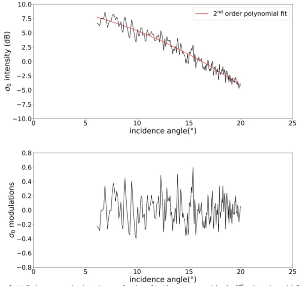
In practice the KuROS radar provides the intensity of the backscattered coefficient as a function of radial distance, integrated onboard over 1 ms. In the post-processing, these signals are post integrated over 33 ms and converted into normalized radar cross section expressed as a function of incidence angle (see Caudal et al. (2014)). A sample obtained after this post processing is shown in Fig (3a). The fractional modulations (plotted in Figure (3b)) are then obtained by removing a 2nd order polynomial fit from the radar cross section signal.

Once the modulations extracted, the modulation spectrum can be computed:

𝑃/ 𝑘, 𝜙 = 𝐹𝑇 𝑚 𝑥, 𝜙 ×𝐹𝑇∗[𝑚 𝑥, 𝜙 ] (10)

Where 𝐹𝑇 stands for the Fourier transform operator, and the asterisk (*) represents the complex conjugate. When applying Eq. (9), we limit the domain to incidence range between 6° and 20°.

The KuROS wave slope spectrum is computed thanks to the equation (8) where the term ?1lQr

?s is estimated

from the 2nd order polynomial fit mentioned above. The wave height spectrum, noted 𝐸 𝑘, 𝜙 , is derived from the wave slope spectrum by:

𝐸 𝑘, 𝜙 =𝑆 𝑘, 𝜙

𝑘O (11)

The full directional wave spectra are estimated by using 30 s data segments which correspond to 1.2 or 2.4 rotations of the antenna, according for its rotation speed. Depending on the acquisition mode of KuROS (alternation between LI and MI antennas or only LI antenna), an estimation of wave spectra is obtained every 3 or 6 km along the flight track for a typical 100 km/s aircraft speed. Considering the along flight advection and the swath of the radar beam, one can consider that the scale associated to our wave spectrum estimation is typically 3 km × 2 km.

With the configuration used for KuROS flights (radial resolution of 1.5 m, elevation footprint dimension of 1000 m in average), wave spectra are inverted in each look direction 𝜙 with a discretization of 128 bins in wavenumber over the interval [0.0049, 0.63 rad.m-1]. The wavenumber resolution is 0.0049 rad.m-1. The wavenumber interval corresponds in the frequency domain to [0.035, 0.4 Hz] when accounting of the wave dispersion relationship in deep water.

The radar technique produces a speckle noise which is removed here by the cross spectra approach proposed by Engen and Johnsen (1995)and recalled in Caudal et al. (2014).

Figure 3. (a) Radar cross section intensity as a function of incidence superposed by the 2nd order polynomial fit. (b) Fractional modulations of the normalized radar cross section as a function of incidence.

In spite of the detrend operation, most of the retrieved spectra exhibit a continuous component at very low wavenumbers (~0.002 rad.m-1_{). In order to suppress this non-physical component, the resulting spectrum is} filtered by looking for a minimum value (or a change of the sign of the derivative) of the spectrum for wavenumbers smaller than a wavenumber limit which is adapt from one flight to another. However, for some cases this method is not efficient, in particular when the wave energy at low frequency is mixed with the continuous component. This happens mainly in long swell cases mentioned in Section 3.2.2.

In the following, the results are also analyzed in terms of frequency spectra are used. For this purpose, KuROS wavenumber spectra are converted into frequency spectra using:

𝐸 𝑘, 𝜙 𝑘 𝑑𝑘 𝑑𝜙 = 𝐹 𝑓, 𝜙 𝑑𝑓 𝑑𝜙 (12)

2.3. Integrated parameters

Directional wave spectra give a complete and detailed information on the distribution of the energy of the waves (or their height) with their wavelength and their direction of propagation. However, for analysis and applications it is appropriate to used characteristic parameters of these wave spectra. The most common ones are the significant wave height (also noted 𝐻w), the frequency peak (𝑓i0,x) and the mean direction (𝜙/0,l),

of the spectra are the angular spread (∆𝜙) and the frequency spread (∆𝑓). They are also important parameters which are governed by the wave hydrodynamics and in particular wave-wave interactions.

In this study, these five parameters have been calculated from the KuROS directional wave spectra expressed as frequency spectra.

The significant wave height 𝐻_w is obtained by calculating the integral of the energy spectrum over all the directions and all the KuROS frequency interval:

𝐻_w= 4 𝐹 𝑓, 𝜙 𝑑𝑓𝑑𝜙 (13)

With 𝐹 𝑓, 𝜙 the directional wave height spectrum, f the frequency. For KuROS and the conditions of observations described here, the domain of integration is limited to frequencies between 0.07 Hz and 0.4 Hz, approximately.

The peak frequency (𝑓i0,x) is defined as the frequency corresponding to the maximum of energy of the

omnidirectional wave height spectrum, which is:

𝐹 𝑓 = 𝐹 𝑓, 𝜙 𝑑𝜙

O] 6

(14) The frequency peak is in practice calculated as the first normalized moment of 𝐹 𝑓 around the peak,

estimated over three frequency bins:

𝑓i0,x= 𝐹 𝑓. ∗ 𝑓. {.l_|}~•€ •‚ .ƒ{.l_|}~•€ „‚ 𝐹(𝑓.) {.l_|}~•€ •‚ .ƒ{.l_|}~•€ „‚ (15)

With 𝑏𝑖𝑛‡_}~•€ the frequency bin corresponding to the maximum of energy of the omnidirectional spectrum.

The mean direction (𝜙/0,l) and the angular spread (∆𝜙) are two parameters which indicate the directional

properties of a wave field. Longuet-Higgins et al. (1963)presented a method to compute these two directional parameters from directional wave riders. These latter provide temporal measurements of the acceleration in three directions, and of 3 angles namely, yaw, pitch and roll. In this approach, the directional distribution is then approximated with a Fourier series truncated to the first five coefficients which are estimated from the co and cross-spectra of temporal series of the different measurements.

𝑎‚ 𝑓 = 𝑄‚O(𝑓) 𝐶OO 𝑓 + 𝐶ŠŠ 𝑓 𝐶‚‚(𝑓) (16)

𝑏‚ 𝑓 = 𝑄‚Š(𝑓) 𝐶OO 𝑓 + 𝐶ŠŠ 𝑓 𝐶‚‚(𝑓) (16’)

With Cnn and Qnm the co and cross spectra expressions:

𝐶

𝑓 =

𝐹 𝑓,

𝑑

𝐶

𝑓 =

𝑘

_{𝐹 𝑓,}

_cos

_𝑑

𝐶

𝑓 =

𝑘

_{𝐹 𝑓,}

_sin

_𝑑

𝐶

𝑓 =

𝑘

_{𝐹 𝑓,}

_sin

_𝑐𝑜𝑠

_𝑑

𝑄

𝑓 =

𝑘𝐹 𝑓,

𝑐𝑜𝑠

𝑑

𝑄

𝑓 =

𝑘𝐹 𝑓,

𝑠𝑖𝑛

𝑑

The first pair of Fourier coefficients is used to calculate the mean direction and the angular spread for each frequency: 𝜙/0,l 𝑓 = arctan 𝑏‚ 𝑓 𝑎_‚(𝑓) (17) ∆𝜙 𝑓 = 2(1 − 𝑟‚ 𝑓 ) With 𝑟‚ 𝑓 = 𝑎‚ 𝑓 O+ 𝑏‚ 𝑓 O (18) (18’) The mean direction and the directional spread are calculated for all frequencies. But in the following, the emphasis is put on the mean direction and directional spread at peak frequency only.

KuROS spectra are symmetrized, so for comparisons with the model data, if the difference between the KuROS mean direction and the model mean direction is larger than 90°, then we add (or subtract) 180° to the KuROS mean direction. The ambiguity is not solved in this study. This could be done with external information such as the wind direction.

There is a lot of way to calculate the spectral bandwidth (Saulnier et al. 2011) but the formula retained for this study is the Blackman and Tukey (1959)formula which use spectrum energy:

∆𝑓 = [ 𝐹 𝑓 𝑑𝑓]

O

𝐹O_{(𝑓)𝑑𝑓} (19)

3. Experimental field campaigns

KuROS data analyzed here have been acquired during two measurement campaigns in 2013 and in 2015. These campaigns are presented in the section below. Different meteorological conditions were encountered as described below. In the present study, KuROS data are compared to wave model data in order to check the performances and the limitations of KuROS. This also challenges the models as KuROS data are acquired at a much better spatial resolution. It enables to better describe small scale variations. Model data are compared to buoy data on a larger data set to check the performances of model data. Buoy data are considered as the reference for the main parameters, especially the significant wave height. In this section the models used for this study are first presented. After that, the two campaigns and the meteorological conditions are presented with illustrations of directional and omni-directional wave spectra representative of the different situations.

3.1. Wave model

Two different wave models of third generation are used. The first one is the Météo-France Wave Model Forecast (MFWAM) based on ECWAM-IFS38R2 code with the ST4 physics (Ardhuin et al. 2010). The second one is the WAVEWATCH-III (WW3) model ((version 4.12 Tolman et al. (2014)).

MFWAM is the French derivative version of the WAM model (Lefèvre et al. 2009) which was the first third generation wave model (The WAMDI Group. 1988). In the configuration used here, it provides directional wave spectra on a longitude and latitude grid with outputs every three hours and with a spectral discretization of 15° in azimuth and with 32 frequency bins in the [0.035, 0.55 Hz] frequency interval. The model was run for the Mediterranean domain, over the period of KuROS observations (February and March 2013) using wind inputs either from a global or from a regional atmospheric model of Météo-France: run1 corresponds to wind forcing from the global ARPEGE model (Courtier and Rochas 1991) with a 10 km resolution; run2

corresponds to wind forcing from the regional French AROME model (Seity et al. 2011) at a 2.5 km resolution. An additional run, called run3, has been performed with the global ARPEGE winds by accounting in the physics of the MFWAM model, for the surface currents. In this case, the current fields have been taken from the global Copernicus Marine Service system with a grid size of 1/4° and with values at 45cm depth. The WW3 model is a third-generation wind-wave model developed by an international team around NOAA (National Oceanographic and Atmospheric Administration) and NCEP (National Centers for Environmental Prediction). The version used in this study is the French version developed by SHOM (Service Hydrographique et Océanographique de la Marine) and Ifremer. It also provides directional wave spectra on a longitude-latitude grid with outputs every hour and with a spectral discretization of 15° in azimuth and with 32 frequency bins in the [0.0373, 0.7159492 Hz] frequency interval. Forcing current is from the MARS2D model (Lazure and Dumas 2008) with a resolution which varies from 2 km in open sea, to 250 m near the coasts. Forcing wind is from ECMWF (European Center for Medium-Range Weather Forecasts) operational analysis and forecasts model at a resolution of 1/8°. For the present work, WW3 fields provided on an unstructured triangular grid are used.

3.2. Campaigns

The KuROS radar data analyzed in this paper have been acquired during two campaigns in 2013 and in 2015. The first campaign was in February-March 2013 in the Lion Gulf in the Mediterranean Sea. It took place during the Hydrological cycle in the Mediterranean Experiment (HyMeX). The second one was in October 2015 in the Iroise Sea near the Brittany coasts during the Prévision Océanique, Turbidité, Écoulements, Vagues et Sédimentologie (PROTEVS) experiment leaded by the French naval service: Service Hydrographique et Océanographique de la Marine (SHOM).

3.2.1. HyMeX campaign

HyMeX is an international program which aims at better understanding the water cycle variability with emphasis on extreme weather events in the Mediterranean basin which is subject to high and extremely variable meteorological conditions (Drobinski et al. 2014). A Special Observation Period (SOP) was organized in February-March 2013 in order to improve understanding of atmosphere-sea interactions in particular in conditions of intense winds.

During this SOP experiment, the French research aircraft ATR42 carried out both in situ measurements in the atmospheric boundary layer (from 30 to 1000 m altitude flight segments) and remote sensing measurements of the oceanic surface with the KuROS radar (at altitude of 2000 and 3000 m). Also, in situ measurements of the oceanic surface have been carried out with the “Lion” buoy system moored at position (42.06N, 4.64E). This system was composed of non-directional Datawell buoy and a Tri-axis directional buoy and has been over flown by KuROS during each flight.

Throughout this campaign, 13 flights have been carried out under two typical meteorological conditions: - Under fetch-limited conditions (9 flights on 9 different days)

- Under moderate to strong alongshore easterly wind conditions (4 flights on 4 different days) Those two typical meteorological conditions are presented hereafter and their corresponding wind fields are shown in Figure (4) for one case of each of these situations.

Figure 4. HYMEX campaign area and typical wind fields corresponding to fetch-limited (left) and strong alongshore easterly wind (right) conditions in the Gulf of Lion (cases of February 15th _{2013 à 12 UTC on the left and of March 6}th ₂₀₁₃

at 12 UTC on the right). Arrows indicate the wind vector and color code is for the wind intensity. Wind fields are from the ECMWF model and are similar to those of the ARPEGE model. The white star represents the Lion buoy position (42.06N, 4.64E).

The directional wave spectra in Figures (5a-b) represent the two typical sea states of the HyMeX campaign. The spectrum on the left-hand side corresponds to a wind sea state. The energy peak is at high wavenumber and the energy peak is spread in frequency and direction. On the right-hand side, the directional spectrum is characteristic of a well-developed sea state. Indeed, the energy peak is at larger wavenumber than for the wind sea wave spectrum (left-hand side). Also, the frequency and the directional spreads are lower than the ones of the wind-sea spectrum. Corresponding MWFAM spectra are shown the Figures (5c-d). There is a satisfying qualitative agreement between the KuROS and the MFWAM spectra. Note that KuROS spectra are more detailed in wavenumber because the resolution of KuROS in wavenumber is higher than the one of MFWAM.

Figure 5. KuROS directional wave slope spectra, on February 15th _{2013 (a) and on March 6}th _{2013 (b), showing the two}

different type of sea states during the HyMeX campaign. Distance from the center corresponds to the wavenumber and polar angle represents the azimuthal direction with the North indicated upward. Spectra are symmetrized because of the 180° ambiguity (see Caudal et al. (2014)). (c) (d) show the corresponding MFWAM spectra. Note that energy color bars are not the same between the two situations.

Fetch limited conditions consist in moderate to strong regional offshore winds which occur during cold outbreaks and are called Mistral (northerly winds) and Tramontane (north westerly winds). According to the ARPEGE atmospheric circulation model, during these 9 flights, offshore wind speeds at 10 m of altitude were from 5 to 17 m/s. Figure (6a) shows an example of KuROS trajectories during a case of fetch limited condition on the 15th of February 2013. The open black squares are the grid points of the model discretized at 10 km and the colored and black squares are all the KuROS measurement points for this flight. The total duration of this flight is 4 hours. In Figure (6a) the multi-colored squared are the positions of the KuROS wave frequency spectra plotted in Figure (6b) with the corresponding color codes on the map (6a). Each spectrum of Fig (6b) correspond to a different fetch distance (from 10 to 120 km). In Figure (6c), collocated MFWAM-run1 spectra are represented with the same color code. Although the shape of the KuROS and

(a) _(b)

MFWAM omnidirectional spectra show some differences, they are in good agreement and show typical behavior of fetch-limited wave growth from the coast to the open sea. With increasing fetch distances, the energy increases, the peak frequency and the spectral frequency width decrease. Also, we clearly observe with KuROS data an overshoot in energy for short fetch spectra with respect to larger fetch spectra as originally observed in the spectra from the JONSWAP experiment (Hasselmann et al. 1973). Indeed, for KuROS spectra, the energy at the peak of the spectrum for a short fetch condition is higher than the energy of a larger fetch wave spectrum, at the same frequency. This phenomenon is hardly visible on the MFWAM spectra in Fig (6c).

Figure 6. Wave height omnidirectional spectra as a function of frequency from KuROS (b) and from MFWAM-run1 (c) under fetch-limited conditions on February 15th _{2013. Each color refers to a measurement point indicated with the same color on the}

map on the left plot (a). The black open squares are the MFWAM ARPEGE version model grid points. The black colored squares show the position of the KuROS data for the same flight, in addition to those shown in color.

In the other typical meteorological situation corresponding to the right part of Figure (4), strong alongshore easterly wind conditions are due to an anticyclonic system located near the coasts of Spain which induces complex winds circulation in the Lion Gulf and strong winds coming from the East that blow along the coasts of France. According to the ARPEGE model, wind speed during these situations was around 20 to 25 m/s except for one day when the wind speed was around 15 m/s, and the anticyclonic system moved towards the Balearic Islands.

Figure (7a) shows an example of KuROS trajectories during the strong easterly wind conditions on March 6th 2013. As in Figure (6), in Figure (7b and 7c) presents subsets of the wave height omnidirectional spectra along the flight track. Here it corresponds to well-developed sea state condition with very high wind speeds (25 m/s according to the ARPEGE model). The evolution of the spectra is different from the example shown in Figure (6), the frequency peak is constant along the flight segment both from KuROS and MFWAM-run1. The energy at the peak of the spectra increases from the southern to the northern part of the segment but this variation is more erratic for the KuROS data than for the MFWAM model spectra. This kind of evolution of spectra indicates that the sea state is a well-developed wind sea. Indeed, using wind information from the model, the wave age is estimated between 0.9 and 3.5, knowing that waves are considered fully developed when their age is more than 1.2 (Donelan et al. 1985).

Figure 7. Wave height omnidirectional spectra evolution of KuROS (b) and of MFWAM-run1 (c) as a function of frequency under strong easterly wind conditions on March the 6th 2013. Each color refers to a measurement point indicated with the same color on the map on the left plot (a). The black open squares are the MFWAM ARPEGE version model grid points. The black colored squares show the position of the KuROS data for the same flight, in addition to those shown in color.

In section (4) below we present an overall analysis of the spectral parameter for all the fetch-limited and

(a) _{(b) (c)}

(a)

3.2.2. PROTEVS campaign

The Iroise Sea is one of the most dangerous sea in Europe for the navigation because this area is characterized by a complex bathymetry and is also subject to intense tide currents with current speeds up to 4 m/s locally, leading to intense interactions between the waves and the currents. In order to better characterize wave-current interactions and storm surge conditions in the Iroise Sea, the SHOM organized in October 2015 the PROTEVS experiment, which combined in situ measurements (wave riders), HF radar observations and the KuROS flights. Five flights have been carried out with KuROS between October 23rd and October 28th of 2015. The area sampled by KuROS during this period is shown in Figure (8). It includes regions close to the shore with islands where surface tidal currents are maximum and also over regions less affected by the current. A Datawell directional buoy was moored at position (48.25N, 5.15W). Another buoy named “Pierres Noires” is also always moored in this area, at the position (48.29N, 4.97W). These buoys were not overflown by KuROS at each flight but the most distant KuROS passage for comparison to the buoys was at approximately 25-30 km. For the study, the data of the “Pierres Noires” buoy are compared with model data because omni-directional wave spectra and directional information were provided.

Figure 8. PROTEVS campaign area and typical current field (from the MARS2D model) corresponding to the low tide condition on October 28th _{at 9h UTC. Arrows indicate the current. White squares are the positions of the wave spectra}

from the five KuROS flights. The white triangle indicates the Datawell buoy position (48.25N, 5.15W). The white star indicates the “Pierres Noires” buoy position (48.29N, 4.97W).

During the KuROS flights, low to moderate wind conditions were encountered with wind speed varying from 3 to 12 m/s (according to the ECMWF model) depending on the day. According the WW3 model, the sea conditions were rather stationary over the 5 days with long swell (between 200 and 300 m wavelength) coming from the west direction. Swell systems were sometimes accompanied by weak wind sea formed by local winds blowing from the North on October 24th 2015 and coming from the South on October 26th and October 28th 2015.

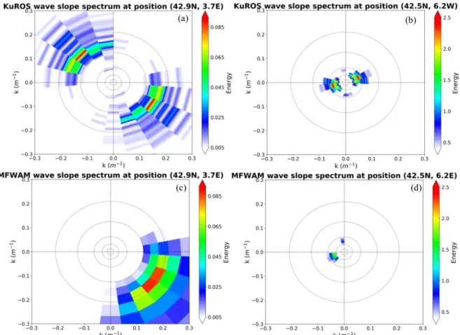
So, during the KuROS flights, two kinds of sea states have been observed. They are illustrated in Figure (9) with two KuROS directional wave slope spectra (a-b) and the two WW3 directional wave slope spectra collocated with the KuROS ones (c-d). The first kind of typical spectrum is plotted in Figure (9a and 9c) and shows a mixed sea condition with a swell component at low wavenumber (0.025 rad m-1) propagating to the East and a wind-sea component at higher wavenumber (0.07 rad.m-1) generated by a wind speed around 10 m/s from South-East. The second type (Figures (9b-9d)) exhibits a pure swell system. The agreement is rather good between the KuROS and the WW3 spectra despite some differences in the energy.

Figure 9. KuROS directional wave slope spectra, on October 26th 2015 (top left) and on October 27th 2015 (top right), showing the two different type of sea states during the PROTEVS campaign. Distance from the center corresponds to the wavenumber and polar angle represents the azimuthal direction with the North indicated upward. Spectra are symmetrized because of the 180° ambiguity (see Caudal et al. (2014)). Bottom left and bottom right plots are the WW3 spectra collocated with the KuROS spectra. Note that energy color bars are not the same between the two situations.

Figure (10) shows the evolution along the flight track for both KuROS (10b) and WW3 (10c) from the coast to the open sea of omnidirectional wave height spectra in the case of October 26th 2015. It shows that there is a mixed sea system with a swell component around 0.08 Hz and a wind sea component around 0.15 Hz.

Figure 10. Wave height omnidirectional spectra evolution of KuROS (middle) and of WW3 (right) as a function of frequency under moderate South wind conditions on October 26th _{2015. On the left, the map of the KuROS point in color}

(each color corresponds to the position of the spectrum). The black open squares are the WW3 model grid points.

Although these two components exist on both KuROS and WW3 spectra, the swell component is more energetic for KuROS spectra than for WW3 spectra, and, on the contrary, the wind sea component is less energetic for KuROS than for the WW3 spectra. Also, the wind sea component is noisier for KuROS, and shows several energy peaks whereas the model indicates a unique energy peak for the wind sea component. Even if the agreement is not perfectly good in terms of energy between the radar and the model, both indicate a mixed sea state and energy peaks are at the same frequencies.

(a) (b)

(c) (d)

In section (4) below, we present an overall analysis of the spectral parameters for all the KuROS measurement points of the PROTEVS campaign.

4. KuROS-model-buoy overall comparisons

Significant wave height, frequency peak and mean direction corresponding to the peak frequency have been calculated from the directional spectra of KuROS data for both campaigns. Then, comparisons have been made with the different data sets of the models. For the HyMeX campaign, the KuROS data set has been compared to the 3 runs of the MFWAM model data detailed in Section 2, and for the PROTEVS campaign, KuROS data set has been compared to the WW3 model data. Also, KuROS and model data have been compared to the buoy data deployed during the both campaigns.

All the data are collocated. The model point is determined as the closest grid point from the KuROS measurement point. The time of the buoy acquisition and the model are the closest one of the KuROS acquisition time. The biggest delay between KuROS and the MFWAM model is 1h30. Between WW3 it and KuROS, the largest delay is only 30 minutes because we have model run every hour.

4.1. Results

Comparisons of 𝐻_w, 𝑓_i0,x and 𝜃_/0,l between KuROS and MFWAM-run2 data for the HyMeX campaign are shown in Figures (11a), (11c) and (11e) respectively.Statistical parameters are detailed in Table 2. Over the whole data set the bias is small (0.07 m) but the standard deviation is significative (0.78 m). The analysis has also been performed by separating in two intervals of 𝐻w larger and lower than 4 m. The agreement is

good for all 𝐻w smaller than 4 m (bias = 0.29 m, standard deviation (std) = 0.52 m), but at larger 𝐻w the

standard deviation becomes larger although the bias is smaller (bias = -0.08 m, std = 0.91 m). The large standard deviation appears for the three comparisons with the different runs of MFWAM (see Table 2) but the standard deviation is more important for the MFWAM-run1 (or run3) data (bias = -0.25 m, std = 1.04 m). So, the higher resolution of AROME (MFWAM-run2) seems to increase the agreement between KuROS and MFWAM 𝐻_w. This is because AROME provides a more detailed wind field with a 2.5 km resolution than the ARPEGE version with its 10 km resolution. It is important to note that all the results obtained with the MFWAM-run1 data are the same as those obtained with the MFWAM-run3 data. So, in the conditions of HyMeX, the current, as considered in the model, has no visible impact on the wave model results. This was more or less expected because the current speed is relatively low in this region (maximum current speeds between 0.2 and 0.3 m/s). In the following, the conclusions for run3 are not detailed because they are similar to those from run1.

Despite the large standard deviation between KuROS and the model at high 𝐻_w, the agreement is rather good for 𝑓i0,x over all sea-state conditions (bias = 0.005 Hz, std = 0.02 Hz).

Concerning the mean directions, the agreement is rather good for all directions in the East to South-West (between 90° to 200°) sector (bias = -2°, std = 16°). The measurement points in this sector correspond to fetch-limited conditions. In the opposite, directions for waves that are going to South-West and North sector have a larger bias and standard deviation (bias = -7°, std = 19°). These measurement points concern the waves with longer wavelength under non-fetch-limited conditions. This difference appears also for the MFWAM-run1 study.

Similarly to the case of the 𝐻w comparison, the higher resolution of AROME (MFWAM-run2) reduces some

discrepancies with respect to run1 corresponding to the ARPEGE wind resolution especially for the 𝐻w, as

explained before, and also for the mean direction parameter in fetch-limited conditions (bias = -13°, std = 22° for the ARPEGE version and bias = -10°, std = 19° for AROME).

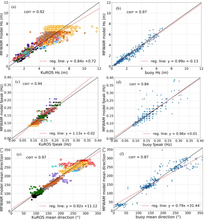
Comparisons between MFWAM-run2 wave parameters and the Tri-axis buoy wave parameters have also been carried on more than 1 month of observations between the 5th of February and the 15th of March 2013. They are shown in Figures (11b), (11d) and (11f). The results indicate a good agreement for 𝐻_w (biais = -0.15 m, std = 0.42 m), for 𝑓i0,x (bias = 0.004 Hz, std = 0.029 Hz) and for 𝜙/0,l despite of a more important

standard deviation than for the KuROS-MFWAM comparisons (bias = -3.5°, std = 43°). For 𝐻_w larger than 4 m, the standard deviation is significantly smaller than the KuROS-MFWAM comparisons (std = 0.56 m). This seems to indicate that the standard deviation of 𝐻w between KuROS and MFWAM at large 𝐻w (> 4 m)

In contrast, for the mean direction, the standard deviation between buoy and MFWAM data is more important than between KuROS and MFWAM (std = 43° and std = 17°, respectively). Regression line and correlation coefficient indicate that KuROS and model data have a better agreement than the model data with the buoy data. At this stage it is however difficult to attribute this discrepancy to inaccuracies in the model or in the buoy data.

Figure 11. Overall comparisons of the MFWAM-run2 principle wave parameters (𝐻w, 𝑓i0,x and 𝜙/0,l) during the HyMeX

campaign with the KuROS (left-hand side) and the Tri-axis buoy (right-hand side) data. In Figures (a), (b) and (c) there are 1271 measurement points. Each color represents one flight. Star symbols are for flights in fetch-limited conditions, open circles are for flights in easterly high wind conditions.For reminder, buoy data are analyzed over 1 month between the 5th

of February and the 15th _{of March 2013. For the buoy comparison, there are 307 measurement points.}

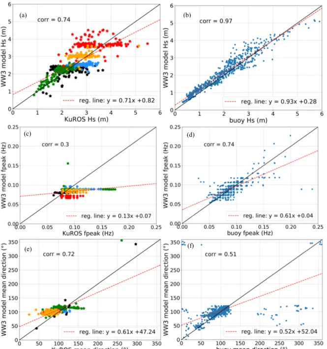
The same study has been carried out for the PROTEVS KuROS data set, but comparisons are made with the WW3 model instead of MFWAM. Comparisons are shown in Figure (12). 𝐻w comparison (Figure (12a))

shows a good agreement for moderate values and a larger dispersion for higher sea states. It is almost the same result as for the HyMeX campaign: the standard deviation for all the measurement points is 0.51 m which is close to the standard deviation of the measurement points of the HyMeX campaign with 𝐻_w lower than 4 m (0.52 m).

(b) (a)

(c) (d)

The agreement on the frequency peak is not as satisfying as for the HyMeX campaign. KuROS frequency peaks have larger variations than the WW3 frequency peaks. The sea states of the PROTEVS campaign are essentially swell system sometimes crossed with wind sea system (blue and green star flights). The scatter is due to these crossed sea systems because KuROS spectra have wind sea component more energetic than the swell component whereas the swell system is more energetic than the wind sea component for the WW3 spectra (see Fig. (10)). There is also a systematic underestimation of KuROS for the frequency peaks of one of the flights (identified by the red star symbol in Fig. (12)). This case is a pure swell sea state with waves of 300 m of wavelength according to the WW3 model. This type of sea state is likely a limiting case for KuROS. It will be discussed in the Section 4.2 below.

Comparison of the mean direction at the peak indicates also a significant standard deviation of KuROS values (bias = 4.6°, std = 14.4°). The regression line and the correlation coefficient indicate also that the comparison is not as good as the HyMeX comparison (corr = 0.72). This discrepancy may be due to the disagreement on the frequency peak between KuROS and WW3 due to differences in the swell and mixed sea identification mentioned here above.

Comparisons between WW3 wave parameters and the “Pierres Noires” buoy wave parameters have also been carried out for a 1-month data set encompassing the PROTEVS campaign (3- 31 October 2015). They are shown in Figures (12b), (12d) and (12f). The results show a good agreement for 𝐻w (bias = 0.14 m, std = 0.30

m). Bias and standard deviations are in Table (3). As for the HyMeX campaign, this conclusion comforts in the fact that the discrepancy between the radar and the model at high values of 𝐻w are due to a scatter in the

KuROS data. The agreement for the peak frequency is rather good except for two points that are around 0.2 and 0.25 Hz for the buoy whereas the model indicates peak frequencies around 0.08 Hz. Those two points have been recorded on the 26th of October in the morning. This is the same day as the green star flight in Figure (12c). KuROS and the buoy both indicate a wind sea more energetic than the swell system. Peak frequencies from KuROS are lower than from the buoy, but this can be explained by the different fetch distances in this situation of southerly to east-southerly winds. The agreement between buoy and WW3 for the mean direction is also satisfactory, although there are some outlier points. They correspond to cases for which the buoy indicates a dominant high frequency wind sea (> 0. 25 Hz) whereas the model indicates a dominant swell system. These points are also outliers in Figure (12d) but are not visible in the plot because of the scale of the graph. That is why correlation coefficients are lower than for the HyMeX comparisons.

Figure 12. Overall comparisons of the WW3 principle wave parameters (𝐻w, 𝑓i0,x and 𝜙/0,l) during the Iroise campaign

with the KuROS (left-hand side) and the “Pierres Noires” buoy (right-hand side) data. In Figures (a), (b) and (c) there are 586 measurement points. Each color represents one flight. For reminder, buoy data are analyzed over 1 month between the 3rd _{of October and the 31}th _{of October 2015. For the buoy comparison, there are 683 measurement points.}

4.2. Discussions on main spectrum parameters

Overall comparisons between the KuROS and the MFWAM-run2 data for the HyMeX data set indicate that the agreement is rather good especially for the fetch-limited cases (stars in Figures (11a), (11c) and (11e)). However, a significant scatter appears for 𝐻w larger than 4 m. Correlatively, comparison of 𝐻w between

MFWAM and buoy data shows a good agreement even for 𝐻w larger than 4 m (bias = -0.15 m, std = 0.42 m).

From this double comparison, we conclude that the standard deviation in the former cases is probably due to the KuROS radar data. Measurement points that have 𝐻_w larger than 4 m show also the least disagreement for 𝜙/0,l compared to the other measurement points. The cases for which comparisons are less satisfying

correspond to well-developed sea state conditions with ocean waves around 200 m of wavelength. For PROTEVS data set, which corresponds to either pure swell cases or mixed swell/wind sea cases, we also find the same type of standard deviation on 𝐻_w and mean direction. In addition, some bias is found for the peak frequency and explained by a different relative energy of wind sea versus swell wind between model and

(a) (b)

(c) (d)

(f) (e)

As presented in section 2.2, the main limitations for the inversion of wave spectra from KuROS are the assumptions on wave slopes, and on correlation length (respectively wavelength) of the ocean waves, which must be small compared to the azimuth (respectively elevation) dimension of the radar footprint. These two factors may lead to some non-linearity in the relationship between radar signal spectra and wave slope spectra.

The significant slope (_“’_

}~•€ with 𝜆i0,x the dominant wavelength) have been estimated from the model in

order to check the assumption of the wave slope. In average, local slopes of the waves, as given by the model, are of 3 % for fetch-limited and strong easterly wind conditions. This value is just at the limit of validity for the linearity. However, as explained above, comparisons under fetch-limited conditions are satisfying, whereas the averaged significant wave slopes are nearly the same between the both conditions. For the PROTEVS data set, the significant wave slopes are between 0.5 % and 1.5 % according to the WW3 model. So, we conclude that the limiting factor is not due to the slopes of the ocean waves for the situations met by the KuROS radar during the field campaigns.

The second assumption that can possibly be a limitation is the size of the footprint compared to length of the waves. Indeed, most of the measurement points obtained during the HyMeX campaign have been acquired at 2000 m of altitude. At this flight altitude, the dimension of the radar footprint is around 700 m in elevation and 300 m in azimuth. The dimension in elevation of the radar footprint is long enough to detect waves of 200 m of wavelength. But in the azimuth direction, the correlation length may be of the order of the footprint dimension. Indeed, using simple simulations of the surface slopes, we found that a swell of 200 m of wavelength simulated with a cos‚” _{angular spreading function induces correlation length perpendicular to}

the propagation direction of 350 m. Correlatively the mean slope in the y direction is also not null. Hence assumption underlying Eq. (7) may be violated. It may bias the retrieved energy of the wave spectrum but can vary from scenes to scenes due to the statistical fluctuation at the surface. Indeed, correlation lengths and mean slopes in the y direction are very fluctuant. This variation could explain the increased standard deviation of 𝐻𝑠 with a mean zero bias.

Finally, a continuous bias is not visible for the comparisons with the KuROS radar data. So, the assumption about the Gaussian shape of the gain pattern does not seem to be a limitation.

In summary, combining the results of both campaigns, we conclude that KuROS provides wave spectra with good consistency with models for cases with ocean waves shorter than about 200 m and that the radar footprint dimension seems to be a limit for longer wave situations.

In the following we concentrate our analysis on additional wave parameters, namely frequency spread and directional spread using a subset of KuROS data corresponding to cases where the hypotheses of the measurement principle cannot be questioned. The selection of the data subset has been done based on the values of mean bias and standard deviation of the difference of 𝐻_w between KuROS and the models analyzed as a function of the frequency peak. By sorting data according to the model peak frequency, all data for which the peak frequency is such that the mean bias of 𝐻w differences is larger than 1 m or the standard deviation

of 𝐻_w differences is larger than 0.8 m are deleted from the data set. As it was expected, it corresponds to measurement points with ocean waves of wavelength higher than 200 m (peak frequency smaller than 0.088 Hz).

4.3. Study of frequency and directional spread

The frequency and angular spread are two parameters that provide interesting information about wave spectra because they are constrained by the physics of the wave (in particular the non-linear interactions). Observations of this kind of parameters are needed to improve and validate the theory and the numerical models.

For this study, ∆𝜙 and ∆𝑓 are estimated using Eq. (18 and 19, respectively) in Section 2.3. ∆𝜙 is computed at the peak of the wave spectrum.

Figures (13a-b) and (14a-b) show these parameters estimated from the KuROS data subset compared to the collocated model values. The same type of comparisons between the Tri-axis buoy and the MFWAM-run2

data are presented in Figures (13c-d) and (14c-d). The data set used for the comparison with the buoy is the same as the one in the Section 4.

From these comparisons it appears that in the conditions of the HyMeX campaign subset (mainly fetch-limited cases),

- the MFWAM model overestimates the frequency width of the spectra compared to KuROS (bias = 0.035 Hz) and also to buoy data (bias = 0.03 Hz) in the same range of frequency spread. Regression lines indicate also the overestimation for both comparisons. So, it is reasonable to conclude that MFWAM generates spectra with energy too widely spread in frequency in these fetch-limited conditions.

- The MFWAM model underestimates the directional spread compared to KuROS (bias = -3.6°) and to the buoy data (bias = -9.3°). Regression lines for both comparisons are similar.

These conclusions are similar for the other MFWAM runs.

During the HyMeX campaign, the airborne radar flew 12 times over the buoy (approximately once per flight). On this limited data set, both the frequency width and the directional spread of KuROS are in good agreement with the Tri-axis buoy data with very small bias (0.0045 Hz on frequency spread, and -2.7° in directional spread).

So, although the standard deviation remains large, and the comparison between KuROS and in situ data is scarce, this triple information from KuROS, MFWAM model and buoy data indicates consistency for the comparisons of MFWAM with KuROS on one side and MFWAM with buoy on the other side. They both seems to indicate that the model fails to reproduce correctly the details of the frequency and the directional properties of the wave spectra in these fetch-limited cases. This may come from some approximations used in the model for the redistribution of energy due to non-linear interactions between different wave components. This results in an insufficient redistribution in directions compensated by a too important redistribution in frequency (and vice-versa).

In the conditions of the PROTEVS campaign, Figure 14 shows that WW3 also overestimates the frequency spread of the spectra compared to the KuROS data set (bias = 0.02 Hz). But in this case, the overestimation of the model spectral width compared buoy data is smaller than in the HyMeX case for the same range of frequency spread (see Fig. (14c)). So, as for the HyMeX campaign, the model overestimates the frequency spread for values lower than 0.12 Hz.

As for the direction spread, similarly to the case the HyMeX campaign with MFWAM, WW3 underestimates this spread compared to both buoy (bias = -7.5°) and KuROS data (bias = -11.7°). Regression lines for both comparisons are also similar and confirm the underestimation.

In summary for the PROTEVS campaign, the analysis on the frequency spread is less conclusive but it seems possible to claim that the WW3 provides too broad distribution of wave energy in directions compared to both KuROS or to buoy data. This conclusion is not depending of the current speed.

Figure 13. Overall comparisons of the MFWAM-run2 wave parameters (∆𝑓 on Figures a-b and ∆𝜙 in Figures c-d) during

the HyMeX campaign with the KuROS (left-hand side, a and c) and the Tri-axis buoy (right-hand side, b and d) data. The red lines represent the regression lines. In Figures (a) and (c) there are 609 measurement points. Each color represents one flight. Star symbols are for flights in fetch-limited conditions, open circles are for flights in easterly high wind conditions. For reminder, buoy data are analyzed over 1,5 months between the 5th _{of February and the 15}th _{of March 2013. For the buoy}

comparison, there are 307 measurement points.

(a) (b)

Figure 14. Overall comparisons of the WW3 wave parameters (∆𝑓 in Figures a-b and ∆𝜙 in Figures c-d) during the

PROTEVS campaign with the KuROS (left-hand side, a, c) and the ‘Pierres Noires’ buoy (right-hand side, b, d) data. The red lines represent the regression lines. In Figures (a) and (c) there are 460 measurement points. Each color represents one flight. For reminder, buoy data are analyzed over 1 month between the 3rd _{of October and the 31}th _{of October 2015. For}

buoy comparison, there are 683 measurement points.

KuROS - MFWAM run 1 KuROS - MFWAM run 2 KuROS - MFWAM run 3 KuROS - WW3

Parameter bias std bias std bias std bias std

𝐻_w -0.0051 m 0.89 m 0.067 m 0.78 m -0.0053 m 0.89 m 0.076 m 0.51 m 𝐻w < 4 m 0.36 m 0.60 m 0.29 m 0.52 m 0.34 m 0.60 m / / 𝐻w> 4 m -0.25 m 1.04 m -0.08 m 0.91 m -0.25 m 1.04 m / / 𝑓i0,x -0.00063 Hz 0.011 Hz -0.0018 Hz 0.013 Hz 0.00043 Hz 0.011 Hz -0.0093 Hz 0.02 Hz 𝜙/0,l -2° 18° -5° 17° -3° 19° 4.6° 14° ∆𝑓 0.030 Hz 0.039 Hz 0.035 Hz 0.041 Hz 0.033 Hz 0.042 Hz 0.025 Hz 0.040 Hz ∆𝜙 -2.0° 5.6° -3.6° 6.8° -1.1° 5.5° -12° 13°

Table 2. Bias and standard deviations (std) of the comparisons of the wave parameters between KuROS and the models. Number of points for KuROS-MFWAM comparisons is: 1271 points of 𝐻𝑠, 𝑓i0,x, 𝜙/0,l and 307 points for Δf and Δ𝜙. Number of points for KuROS-WW3 comparisons is: 586

points 𝐻𝑠, 𝑓i0,x, 𝜙/0,l and 460 points for Δf and Δ𝜙.

(a) (b)