HAL Id: halshs-00966312
https://halshs.archives-ouvertes.fr/halshs-00966312
Preprint submitted on 26 Mar 2014
HAL is a multi-disciplinary open access
archive for the deposit and dissemination of sci-entific research documents, whether they are pub-lished or not. The documents may come from
L’archive ouverte pluridisciplinaire HAL, est destinée au dépôt et à la diffusion de documents scientifiques de niveau recherche, publiés ou non, émanant des établissements d’enseignement et de
Development at the border : a study of national
integration in post-colonial West Africa
Denis Cogneau, Sandrine Mesplé-Somps, Gilles Spielvogel
To cite this version:
Denis Cogneau, Sandrine Mesplé-Somps, Gilles Spielvogel. Development at the border : a study of national integration in post-colonial West Africa. 2010. �halshs-00966312�
Development at the border:
a study of national integration
in post-colonial West Africa
Denis COGNEAU
Paris School of Economics Sandrine MESPLE-SOMPS IRD DIAL Univ. Paris 1 Panthéon Sorbonne Gilles SPIELVOGEL
September 2010
Development at the border: a study of national
integration in post-colonial West Africa
∗
Denis Cogneau
†, Sandrine Mespl´e-Somps
‡, and Gilles Spielvogel
§September 20, 2010
Abstract
In Africa, boundaries delineated during the colonial era now divide young in-dependent states. By applying regression discontinuity designs to a large set of surveys covering the 1986-2001 period, this paper identifies many large and signif-icant jumps in welfare at the borders between five West-African countries around Cote d’Ivoire. Border discontinuities mirror the differences between country av-erages with respect to household income, connection to utilities and education. Country of residence often makes a difference, even if distance to capital city has some attenuating power. The results are consistent with a national integration process that is underway but not yet achieved.
Keywords: Institutions, geography, Africa. JEL classification codes: O12, R12, P52
∗We thank Charlotte Gu´enard and Constance Torelli for their participation in the first stage
of this study. For historical archives, excellent research assistance from Marie Bourdaud and Ang´elique Roblin is gratefully acknowledged. We thank the National Institutes for Statistics of Burkina Faso, Cote d’Ivoire, Ghana, Guinea and Mali for giving us access to the surveys. We last thank seminar participants at Oxford (CSAE), The Hague (ISS), Clermont-Ferrand (CERDI), and Paris (CEPR/EUDN/AFD Conference and PSE), and especially Jean-Marie Baland, Luc Behaghel, Michael Grimm, Marc Gurgand and Sylvie Lambert. The usual disclaimer applies.
†Corresponding author. Paris School of Economics IRD, and DIAL. PSE, 48 bd Jourdan
-75014 Paris. Tel: +33-143136373. E-mail: cogneau@pse.ens.fr
‡Institut de Recherche pour le D´eveloppement (IRD), UMR 225 DIAL, Universit´e Paris
Dauphine. E-mail: mesple@dial.prd.fr
§Universit´e Paris 1 Panth´eon-Sorbonne, UMR 201 ”D´eveloppement et Soci´et´es” (Universit´e
Development at the border: a study of national
integration in post-colonial West Africa
September 20, 2010
1
Introduction: The question of African boundaries
State consolidation is widely considered as the most important issue for the de-velopment of Africa, and state failure is often related to the difficulties raised by artificial boundaries. For the most part, the boundaries between African countries have been fixed by European colonial powers at the end of the 19th century, after the 1884 Berlin Conference and the so-called ”Scramble for Africa” (Brunschwig, 1972; Packenham, 1991; Wesseling, 1991). They were to a large extent arbitrar-ily delineated; nevertheless they have been hardly modified since then (Brownlie,
1979).1
Are African borders still weak and abstract lines drawn on a map, or have they become strong and real discontinuities revealing an ongoing process of na-tional integration? Are border neighboring regions alike or do they rather mirror their respective national core? These are the questions we ask in this paper. 1According to Alesina, Easterly and Matuszevski (2006), 80% of African borders follow
lat-itudinal or longlat-itudinal lines. During the colonial period, borders’ modifications mainly arose from the World Wars and the loss of colonial possessions by Germany then Italy. In the post-independence period, the secession of Eritrea from Ethiopia constitutes the only significant ex-ception to the general rule of borders’ intangibility.
The identification of the impact of national institutions on economic outcomes is traditionally based on correlations extracted from macroeconomic data (e.g., La Porta et al., 1999; Acemoglu, Johnson and Robinson, 2002), whose limitations are more and more discussed (e.g., Pande and Udry, 2005). Recent works exploiting province or district-level data within large nations or empires prove that a higher level of disaggregation, both on outcomes and institutions, can provide new inter-esting results (e.g., Banerjee and Iyer, 2005; Huillery, 2009). Here, drawing from a set of large sample household surveys undertaken around 1990, we compare the development outcomes of neighboring localities on both sides of the borders be-tween Cote d’Ivoire, Burkina Faso, Ghana, Guinea and Mali. We examine a large array of variables including monetary welfare, connection to utilities, and adult literacy. We assess the impact of migration flows in and out border regions. Last, we use regression discontinuity designs to test for the insulating power of national boundaries.
The literature on Africa’s development displays a variety of arguments re-garding the role played by boundaries between states. A first bunch of contribu-tions conveys the idea of boundaries weakness and porosity. According to Herbst (2000), the guaranty from the Organization for African Unity (OAU) and the United Nations discourages African states from investing in territorial control; who holds the capital city holds the country, ”the broadcast of power radiating out [from the political core] with decreasing authority” (Herbst, p.171). These ”territory-states”, as opposed to nation-states, are somewhat in keeping with pre-colonial political institutions, in a persistent context of low population density. Furthermore, African boundaries ”dismember” ethnic groups who still today live on both sides of borders (Englebert, Tarango and Carter, 2002). Common lan-guages and cultures contribute to informal cross-borders flows of goods, money and people. According to Easterly and Levine (1998), growth in African countries is strongly influenced by neighbors, meaning that boundaries do not work as a
powerful insulating device.2 Finally, another class of papers states that climate,
terrain or ecology, rather than national institutions, have a large direct influence on economic outcomes, especially in an agrarian context (e.g., Bloom and Sachs, 1998): in that case again, borders should be very much invisible.
A second strand of the literature rather stresses the salience of national idiosyncrasies and a centripetal effect of boundaries. As noted by Robinson (2002) in his review of Herbst’s book, the boundaries of Latin American countries, who became independent at the beginning of the 19th century and are now considered as well-established nation-states, also exhibit some degree of arbitrariness. Besides, ethnic salience is no fate: Posner (2004) studies two ethnic groups living across the border between Malawi and Zambia, and argues that ethnic identification varies with the demographic size, hence the political weight, of each group. Miguel (2004) also suggests that the promotion of national identity by the Tanzanian leader Julius Nyerere succeeded in canceling out the negative impact of within-village ethnic heterogeneity on public goods provision that one observes in neighboring
villages of Kenya.3 Finally, at the macroeconomic level, the inequality of income
between African countries is larger than usually thought: in Schultz (1998), one can observe that the log variance of GDP per capita in PPP reaches 0.415 in 1989 Africa (including North Africa), i.e. by far the highest level among all other regions 2A related political economy literature considers that African boundaries are strong enough
to be a major impediment to growth, in that they create heterogeneous political entities, but too weak to generate homogenizing forces for national integration. They however do not provide a clear-cut prediction on borders’ insulating power. Easterly and Levine (1997) explain ”Africa’s growth tragedy” by ethnic heterogeneity among national states, and Englebert, Tarango and Carter (2002) also argue that states ”suffocate” because of political culture heterogeneity. Like-wise, Alesina, Easterly and Matuszevski (2006) contend that African boundaries have created ”artificial states” whose difficult political economy hampers growth.
3In comparison with Miguel’s paper, this one looks at differences in development levels rather
than differences in ethnic heterogeneity influence, on a set of five countries instead of two, and in Western, rather than Eastern, Africa. It also provides a more thorough testing of cross-border discontinuities.
in the world. Furthermore, this number is twice as high as in 1960 (0.213); the only other region that records such an intercountry divergence during the same period is East Asia (from Korea to Myanmar), although at much lower levels (from 0.067 to 0.197). Of course, income divergence between African countries could only reflect the divergence of their centers, not so much of their border regions; its is
however difficult to reconcile it with a strong influence of neighbors on growth.4
Section 2 sets down the analytical methodology and argues that the African borders we study can be seen as ”natural experiments” that make it possible to estimate, at least locally, the causal treatment effect of living in one country or another.
Section 3 presents our compilation of survey and geographical data, and how we implement our border treatment effects estimators.
In section 4, we compute simple mean differences between border districts, and show they are often in keeping with national level differences, even though pretty much attenuated in many cases. Border differences in welfare also follow the relative ups and downs of national macroeconomic conjunctures. Besides, we reveal the long-term divergence in adult literacy between Cote d’Ivoire and the four other countries after 1960; strikingly enough, for cohorts born in border districts before independence, only the already existing international border with Ghana made a significant difference. We observe migration flows in and out border regions but show that their influence on comparative development is modest.
In section 5 at last, we implement regression discontinuity designs that for-mally test for the existence of a significant jump in outcomes at national borders; these tests robustly confirm the significance of many but not all border differences 4The insulating power of boundaries is not necessarily for the good: the ’balkanization’ of
Africa is often considered as preventing the exploitation of returns to scale, despite efforts of regional trade integration. However the impact of full political integration is different from a simple size merger, and it can be less easy for two countries to have convergent interests in the former: in Africa, Spolaore and Wacziarg (2005) find only one country-pair for which the cancelation of political borders would be mutually beneficial, i.e. Mali and Niger.
in terms of consumption expenditures, connection to electricity, access to water and adult literacy. It is in the peripheral areas that are the most remote from the countries’ centers (Guinea/Mali/Cote d’Ivoire) that we find border discontinuities to be blurred or erased: the above mentioned ”radiating core” model from Herbst finds here an illustration. Otherwise, when looking at borders that divide coun-tries with close development levels and whose distances to both capital cities are also close (Cote d’Ivoire/Ghana and Mali/Burkina Faso), we still find significant discontinuities whose size and sign may vary with the ups and downs of countries macroeconomic climates.
Section 6 concludes: National borders already matter in Africa, and the country of residence makes a difference.
2
Analytical methodology: Borders as experiments
We ask here whether the borders we study are historical ”natural experiments” that have divided territories with initial identical characteristics, so that any ob-served border discontinuity could be attributed to distinct national idiosyncrasies having emerged later on. In more technical terms, do border differences allow to identify ”national treatment effects”? Consider a person born somewhere in the area now named Cote d’Ivoire. What would her welfare be if Cote d’Ivoire had been colonized by the British instead of the French, like Ghana? It is certainly difficult to say, for at least three reasons: (i) the British could have set different institutions to rule Cote d’Ivoire; (ii) Ghana and Cote d’Ivoire merged would not be the same, if only because of market size and general equilibrium considerations; (iii) even if Ghana’s institutions had been kept the same, we have no clue how Cote d’Ivoire initial characteristics would interact with them. Now take a person born in Cote d’Ivoire at the border of Ghana, and imagine the border was some kilometers further. Including this person into Ghana would have a marginal and insignificant impact on Ghana’s institutions and economy. Besides, it is very prob-able that this close neighbor of actual Ghanaian people shares with them the same
geographical constraints and the same anthropological characteristics.
Let Y be some outcome variable (income, connection to electricity, etc.), as observed over a sample of people living in two countries at the same date. Let
C = 0, 1 be the dummy variable indicating the country of residence. Let Yi(0)
be the outcome if and when the individual (or household) i lives in the country
C = 0, and Yi(1) in the country C = 1. Observed outcome reads:
Yi = (1 − Ci).Yi(0) + Ci.Yi(1) (1)
We are seeking to approach E[Y (1) − Y (0)] that is the average treatment effect (ATE) of living in the country 1 rather than in the country 0. A regression discontinuity (RD) design based on distance to the border appears as an obvious
candidate. Let Di stand for the distance to the border of the locality of residence,
positively signed for country 1 and negatively signed for country 0, so that: Ci =
1{Di ≥ 0}.
2.1 Required assumptions for a border RD
Under the assumption that E[Y (0)|D = d] and E[Y (1)|D = d] are continuous
in d, limd→0+E[Y |D = d] − limd→0−E[Y |D = d] provides an estimation of the
average treatment effect at the border (i.e. at D = 0) (Hahn, Todd, Van Der Klauw, 2001). It is the so-called ”sharp” RD estimator. As Lee (2008) argues in another context, this continuity assumption is difficult to assess and impossible to test. Lee’s reformulation elucidates the conditions under which a RD replicates a random assignment around the threshold D = 0. From now, we refer to Lee’s reformulation. Assume Y is generated by a partially unobservable random variable
W : Y (0) = y0(W ) and Y (1) = y1(W ). W represents individuals, households
or localities ”type” with respect to Y . Last, let F (d|w) stand for the cdf of D conditional on W . Lee’s conditions are as follows (Lee, 2008, pp.679):
(i) F (d|w) is such that 0 < F (0|w) < 1
of W
Condition (i) requires that D can be written D = Z(W ) + e where Z is the predictable component of D and e an exogenous random chance component, so that the probability of receiving treatment is somewhere between 0 and 1 for each type. Condition (ii) implies that conditional density f (d|w) is continuous in d at
d = 0. In our case, this implies that the probability of being allocated on either
side next to the border are the same for each ”type” of individuals w. However, in the overall population, D can be arbitrarily correlated with Y (0) or Y (1); Y may also be directly generated by D, in addition to W (Lee, 2008, p.680). Under these
conditions, the RD estimand is a weighted average of the difference y1(w) − y0(w)
for each type w, with weights equal to the probability of being close to the border:
f (0|w)/f (0).5
At the locality level, these conditions require that border localities are not sorted by ”types” w between the two countries. This randomness of distance to the border stems from the historical hazards of boundaries alignment during the colonial period, that we document thereafter.
At the individual level, Lee’s conditions require that people do not ”manip-ulate” their distance to the border through migration, thus affecting their locality of origin ”type”. It is typically an issue for embodied outcomes like human
cap-ital. International migration based on y1(w) − y0(w), or more generally on w, is
obviously the worst case. However, even internal migration flows based on w are a source of bias, because the center of one country can be more attractive than the other for a given type w (for instance, more good schools or good jobs in Abidjan than in Accra). In section 4, we correct for migration bias by computing mean differences between border natives rather than between border residents.
As we do not observe types w we cannot test directly for the validity of these assumptions, namely that the distribution of the ”types” w is the same on both 5Another obvious condition is to have a non empty border, i.e. f (0) > 0 where f (d) is the
sides very near the border. However, as Lee argues, we can test for the absence of discontinuity in the distribution of predetermined observable variables X, like geographical or anthropological variables. We perform this kind of test in section 5. We also check the continuity of the density f (d) at d = 0.
Due to differences in countries’ shape and spatial organization, a specific variable has only few chances to pass this test: the distance to the country capital
city.6 Herbst’s model of radiating core cited in introduction justifies granting a
special attention to this variable. We can think of estimating directly this model by introducing the distance to the capital city as a control in the RD estimation. However, the interpretation of this kind of estimates would be highly heroic, as it is difficult to think of any real world experiment that would simulate a large 200 or 300 kilometers move of the capital city of any of these countries. In 1983 Cote d’Ivoire official administrative capital indeed became Yamoussoukro, but Abidjan still remained by far the largest city in terms of population and income. It can also be argued that for a locality within the border region the counterfactual impact of being annexed by the neighboring country indeed includes a change of capital city, and consequently a jump in the distance to it. For instance, reduced distances to the core are a structural advantage of small size countries that should not be discarded from our estimates. The RD border treatment effect is anyway local; it cannot be read as the differential advantage of dwelling or being born in one country, under a ”veil of ignorance” that would hide the exact place of residence or of birth. In particular, differential discrimination by the central states against some border regions also enter in our estimates. Non-local national treatment effects, or even their difference, cannot be identified, and one can doubt they have any meaning at all.
6For instance, if we consider the Cote d’Ivoire borders with its four neighbors Ghana, Guinea,
Mali and Burkina Faso, they are on average in our samples respectively 236, 566, 637 and 528 km away from Abidjan, against 346 km from Accra, 639 km from Conakry, 302 km from Bamako and 368 km from Ouagadougou. The difference is by far the highest in the case of the border with Mali.
2.2 Historical background and arbitrariness of borders
To further comfort the RD assumptions, we document the alignment of the boundaries we are interested in, drawing from the historical literature and from a
dedicated research in French colonial archives.7 Hargreaves (1985) confirms that
the drawing of boundaries in Western Africa was arbitrary to a large extent. The data collected by Englebert, Tarango and Carter (2002) indicate the presence of
the same ethnic groups on both sides of each border.8 We additionally test for
geographical and anthropological continuity at borders using our survey data (see section 5). In the case of the border of Cote d’Ivoire with Ghana, long-lasting negotiations between the two colonial powers finally resulted in partitions of pre-colonial political entities in the middle part of the border (Gyaman, Indenie, Sefwi); in its southern part (Sanwi), a rebelion unsuccessfully challenged the border align-ment after independence. The three other borders of Cote d’Ivoire are much less clearly demarcated on the field, however they were never contested or challenged. The hazards of French conquest and of the wars against the Almami Samori Ture at the end of the 19th century very much presided to the boundaries alignment within the French Empire; they also resulted in partitions of some former political entities (Kenedugu, Kong and Bouna kingdoms). Those borders were only sta-bilized after World War I; the border with Burkina-Faso (Haute-Volta) was even erased between 1932 and 1947, and then redrawn in its 1919 version. We also use French data on these border regions during the early colonial era (1910-1928), and explore differences in initial conditions between the seven out of eight border areas that pertained to the French empire: Pairwise comparisons do not reveal signif-icant differences in initial conditions between border sides, whether in terms of
indigenous population density, European settlement or trade tax revenue.9 Hence
7Appendix A provides detailed descriptions of the border areas involved in our estimations,
as well as illustrations of the randomness implied in the alignment of these boundaries during colonial times.
8Data is accessible at http://www.politics.pomona.edu/penglebert/, accessed July 8, 2009. 9See table A.1 in appendix A.
we can be fairly confident that present-day national boundaries do not divide areas that were already different in pre-colonial or early colonial times.
3
Data and implementation of border RD estimators
3.1 Data on development outcomes
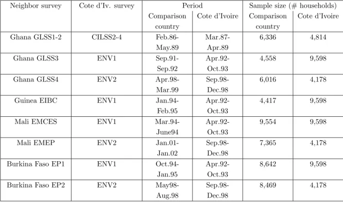
We gather a large database made of 14 multi-topic household surveys: 5 for Cote d’Ivoire, 4 for Ghana, 2 for both Burkina Faso and Mali, and 1 for Guinea; those surveys were implemented between 1985 and 2001. We divide the time line into three periods: 1986-1989, 1992-1994 and 1998-2001. Table 1 lists pairwise compar-isons between Cote d’Ivoire and one of its neighbors, and provides survey names and household sample sizes. For the sake of space the bulk of this paper focuses on Cote d’Ivoire borders; however, section 5 additionally considers the borders between adjacent Cote d’Ivoire neighbors (Guinea/Mali and Mali/Burkina Faso, and Burkina Faso/Ghana). We summarize here the variables construction, more details being provided in appendix B.
[ Insert Table 1 about here ]
The first surveys for Cote d’Ivoire and Ghana are ”integrated” Living Stan-dard Measurement Surveys (LSMS) designed by the World Bank in the 1980s; the other surveys are inspired from them. In all cases, face-to-face interviews were conducted by trained staff.
We pay a lot of attention to the measurement of outcome variables in order to achieve strict comparability between surveys and countries. We construct a household expenditures variable under a common methodology, including all cur-rent expenditures like food, clothing, transportation, housing and imputed cur-rents, etc., and expenditures for education; we only exclude too infrequent or badly mea-sured expenditures like those in health, durable goods, and transfers. We also extract the value of consumption of own food production (except for Mali 1994),
that we add to household expenditures to obtain our total consumption variable. As surveys sometimes cover periods where price inflation was high, we use monthly data on national consumer price index and express individual household consump-tion in a common base-year (1988, 1993 or 1998). Comparisons of household consumption levels are then made in current dollars at base year exchange rates and prices (1988, 1993 or 1998). Cote d’Ivoire, Burkina Faso and Mali share the same currency unit, the CFA franc, so that conversion in dollar is innocuous. For Ghana and Guinea, we use either the official exchange rate or the parallel market exchange rate as reported by African Development indicators (World Bank, 2008). We check that these survey figures for household consumption are consistent with national accounts figures (appendix B). We also compare non-food budget shares, that are unaffected by base price levels and exchange rates, and should be posi-tively correlated with consumption levels.
We also extract a dummy variable indicating whether the household is con-nected to electricity; we additionally consider a dummy for access to water other than rainfalls or rivers. Those welfare variables involve public investments on the supply side and private income on the demand side.
Finally, adult literacy is measured as the self-assessed capacity to read and to write. There is some influential variation in the question asked (read a newspa-per vs read) that prevents comparison between the 1980s LSMS surveys (for Cote d’Ivoire and Ghana) and the others; we are therefore cautious not to mix or com-pare incomparable sources. We also extract the dummy variable saying whether the individual has ever attended school, and check that its evolution across cohorts is broadly in line with that of adult literacy. In the case of Guinea, we disregard
the literacy variable which is little comparable to others.10
10These surveys are more suited to our purpose than Demographic and Health Surveys (DHS)
that are also available for the same set of countries, some of which also including GPS data. First, income or consumption data is absent from DHS surveys. Second, most individual data on adults is restricted to 15 to 49 years-old women, or to rather small sub-samples of men. Third, the set of DHS surveys for Cote d’Ivoire, the pivotal country of our analysis, is reduced to years
3.2 Geographical data
For all these surveys, the sample designs are regionally stratified and two-stage. Within each strata, a first random draw of primary sampling units (PSUs, or survey clusters) is made among a list of localities or cities sub-sectors established from the most recent national census. After enumeration of households within PSUs, a fixed number of households is then randomly drawn in each. Each cluster contains between 12 and 25 surveyed households. The resulting sample comes with a set of unequal weights attached to each PSU (except in the GLSS1 and 2 surveys which are self-weighted).
Within each survey, we first select border areas using the administrative divisions at hand (see figure B.1 in appendix B), and compute simple mean differ-ences at borders that are compared to national mean differdiffer-ences, in section 4. We tighten a bit this selection by excluding the districts whose all survey PSUs are too far, that is more than 100 km away, from the borders; this leads us to restrict our comparisons to the southern parts of the borders of Cote d’Ivoire with Ghana and Guinea. As district and country of birth is known for each individual in Cote d’Ivoire, Ghana and Guinea, we are also able to identify internal and international migrants in these countries. This allows computing mean differences between bor-der natives rather than borbor-der residents. This alternative borbor-der comparison is particularly meaningful when looking at human capital variables across time, as we do in section 4.
In most surveys, excepting Cote d’Ivoire 1998 and Ghana 1992, having the detailed names of survey PSUs allows to code the precise latitude and longitude of even small localities. For each survey cluster, we compute the distance to each border and match its coordinates with NASA datasets that provide geographical indicators: altitude, rainfalls (1984-2001), distance to the closest river within the hydrological basin. Again, more details about variable definition and construction
1994 and 1998, with a very small sample (2,100 households) for this latter year; in the case of Guinea, the first DHS is for 1999.
are provided in appendix B. Thanks to this geo-referencing, we abstract from each country’s administrative divisions and we are able to implement regression discontinuity designs in section 5.
3.3 Implementation of border RD estimators - Optimal bandwidth
and Placebo RDs
To implement the border RD estimator described in section 2, the regression func-tions E[Y (1)|D = d, C = 1] and E[Y (0)|D = d, C = 0] must be estimated around the border point D = 0. The rather small number of survey clusters (localities) on both sides of the border precludes using more flexible but slowly converging non-parametric estimators. We therefore need to add parametric assumptions, as is also very often done in the literature.
The simplest (and strongest) one is to assume that E[Y |D = d] is constant in administrative districts next to the border. This is what we do in section 4, where we simply compute simple mean differences between residents or natives of border districts. This assumption also allows us to exploit some survey data where
the exact location, and hence distance to the border, are not available.11
However, it is certainly debatable that outcomes could be independent from the distance to the border, even within some range. First, localities that are far from the border are also more often closer to the country center, and their expected benefit of being aggregated to the center may be greater than for peripheral lo-calities. Second, distance to the border can be correlated to both observable and unobservable characteristics that also influence outcomes, in particular geography or anthropology. In section 5, to relax this assumption of invariance, we estimate the two regression functions E[Y (1)|D = d, C = 1] and E[Y (0)|D = d, C = 0] by locally linear regressions within a large set of bandwidths:
11Of course, even if outcomes vary with the distance to the border, the magnitude of such
border differences is still revealing of how much border regions look like each other, and may still be contrasted with country mean differences. But it can not be interpreted as the causal effect of the country of living.
Y = γ(h).C + α0(h) + β0(h).D + [β1(h) − β0(h)].C.D + ε (2)
for −h ≤ D ≤ h, with h ∈ {50, 55, 60, ..., 145, 150}.
Like in section 2 notations, C = 0, 1, is the country of residence (e.g., C = 1 in Cote d’Ivoire, 0 in other countries), and D is the distance to the border: C = 1{D ≥ 0}. In the case of discrete outcomes, like connection to electricity, we use a probit specification instead of a linear specification, and in the case of non-food expenditures share, that ranges between 0 and 1, a logistic transformation (ln(x) − ln(1 − x)) is applied; the standard errors of border discontinuities are then computed using the delta-method. Errors (ε) are always clustered by surveys PSUs.
Regarding the choice of the bandwidth h, we implement the ”leave one out” cross-validation procedure described in Lee and Lemieux (2009), and inspired from former contributions of Ludwig and Miller and Imbens and Lemieux (Lee and Lemieux, 2009, pp.40-43). The idea is to predict by linear regression the
out-come Yi of observations i close enough to the cutoff (Di ≤ ∆), while using only
observations on the relevant side of i: Di − h ≤ D < Di if i is on the left of
the cutoff (in our case Di < 0 and Ci = 0), or alternatively Di < D ≤ Di + h
if i on the right of the cutoff (i.e. Di ≥ 0 and Ci = 1). The optimal
band-width then minimizes the average prediction error: hoptCV = arg minhCVY(h), with
CVY(h) =
P
|Di|≤∆(Yi− ˆY (Di))
2.
In the case of the border of Cote d’Ivoire with Ghana, this procedure proves a bit difficult to apply because of a large spatial heterogeneity: Abidjan, the capital city of Cote d’Ivoire, is 100 km away from the border, and its marginal inclusion
in the samples used for computing local predictors ˆY (Di) results in large increases
in prediction errors and hence in CV (h) level. In appendix C, figure C.4 plots
CVY(h), for Y = cash expenditures per capita, against h with limit distances ∆ =
25, 50 and 100 and for each border. With the Ghana border, whatever the subset of observations we select, Abidjan is responsible for a hump in the CV criterion whose
location and width change with the value of ∆. This characteristic of the Cote d’Ivoire/Ghana border at least suggests that Abidjan should be excluded from the computation of equation (2), and hence that bandwidths strictly lower than 100 km should be preferred. From the subset with maximum distance ∆ = 25 and with the
constraint h < 100, we determine hoptCV = 80. With the other borders, the CV (h)
criterion reveals much less sensitive to the choice of ∆. We then straightforwardly
select hoptCV for ∆ = 100. The CV (h) minima all point to rather large optimal
bandwidths: respectively 130, 120 and 135 kilometers for the borders with Guinea,
Mali and Burkina Faso.12
Alternatively to the determination of an optimal bandwidth, we also plot the estimated border discontinuity, γ(h) of equation (2) against all possible bandwidth
h between 50 km and 150 km, in order to check its robustness with respect to
bandwidth choice.
For the bandwidth hoptCV whose determination has just been discussed, we also
run ”placebo RDs” that shift the border by a given number of kilometers k. We
define D(k)= D + k and C(k) = 1{D(k) ≥ 0} and successively run:
Y = γ(k).C(k)+ α(k)0 + β0(k).D(k)+ [β1(k)− β0(k)].C(k).D(k)+ ε (3)
for −hoptCV ≤ D(k) ≤ hopt
CV and k ∈ {−100, −95, ..., 0, ..., 95, 100}. By plotting γ(k)
against k we can then check for the existence of discontinuities at other cutoffs than the actual border. In the cases where a significant border discontinuity is
found (i.e. γ(0) significantly different from zero), we check in particular that the
discontinuity fades away on each side for ”high enough” absolute values of k like
|k| = 25 km, i.e. γ(−25) = γ(25)= 0.
4
Border differences versus national differences
12As for the four other borders we consider later on, i.e. Guinea/Mali in 1993-94, Burkina
Faso/Mali in 1993-94 and 1998-2001 and Burkina Faso/Ghana in 1998, we apply the same method with ∆ = 100 and find respectively hoptCV=75, 125, 125 and 105.
We start our empirical analysis by looking at district level information, i.e. we draw comparisons between the means in outcomes of administrative districts located on both sides of a given border. As already mentioned, this simple procedure has two advantages: first, it allows including survey years for which the precise location of surveys PSUs is unknown (Cote d’Ivoire 1998 and Ghana 1992); second, for some borders and years, it allows the calculation of districts of birth (rather than of residence) mean differences, hence correcting for some of the bias attached to migration.
The figures 1 and 2 display on a map the means of cash expenditures per capita and the rates of connection to electricity for the period 1992-94. The two maps isolate the administrative border areas from the rest of the countries. Let us underline that the 1992-94 period is the worst of all for Cote d’Ivoire, as it corresponds to the climax of the economic crisis that opened in 1989 and closed with the CFA franc devaluation in 1994. Still, these figures illustrate that the higher development of the Cote d’Ivoire country center translates to peripheral border districts. Around the year 1993, we estimate national levels of cash ex-penditures per capita to be 395$ in Cote d’Ivoire against 222$ in Ghana, 217$ in
Guinea, 113$ in Burkina-Faso and 174$ in Mali.13 Contrasts between border
dis-tricts are statistically significant, and very close in magnitude, in three cases out of four: with Ghana (+93$ at the advantage of the Cote d’Ivoire side), Burkina Faso (+86$) and Mali (+110$). These are large differences amounting to 50% of border districts income in the case of Ghana, and even 100% in the cases of the two others. Hence, even for the 1993 bad year, on the grounds of monetary welfare or income poverty, people should have preferred to live in Cote d’Ivoire rather than in another neighboring country, or at least should have been indifferent in the case of Guinea. The same conclusion holds with connection to electricity (figure 2): Cote d’Ivoire significantly dominates its three northern neighbors, even Guinea, 13Corresponding figures for total consumption are 478$, 281$, 255$ and 149$ with no number
border districts in these countries being barely connected, whereas the difference is not significant with Ghana. Comparisons for the earlier (1986-89) or the later (1998-2001) periods deliver the same message: better to live in Cote d’Ivoire, even if differences are often attenuated at borders (see detailed tables at the end of appendix B).
[ Insert Figures 1 and 2 about here ]
For comparisons where districts of birth are available on both sides, i.e. with Ghana and Guinea, we can correct for internal migrations in and out border districts, by looking at mean differences between border natives wherever they live in the country, in the spirit of an equality of opportunity approach of welfare. International migrations are negligible in those two cases and are disregarded. Given the higher relative income of Cote d’Ivoire center in all years, these modified comparisons turn even more favorable to this country, without changing the broad picture. Results not presented show that the most salient change occurs for the comparison with 1994 Guinea in terms of electricity connection (+24 percentage points instead of +17).
For Mali and Burkina Faso where district of birth is not recorded, we can still implement an imperfect correction for international migrations: (i) we identify na-tionals of these two countries in the Cote d’Ivoire surveys (we stick to nationality because country of birth is not available in the Cote d’Ivoire surveys for 1992-93 and 1998); (ii) assuming uniform international migration rates across regions of Mali and Burkina Faso, we reweigh these international migrants and include them in the difference in means computation. For males born 1930-80, this proce-dure results in international migrants weighting respectively 6 and 10% in native populations. Here, as Malian and Burkinab`e migrants benefit from better living conditions in Cote d’Ivoire, putting them back in their country of origin slightly attenuates the estimated national and border contrasts; however, the correction for internal migrations from Cote d’Ivoire northern borders to the country center
plays in the other direction.
Estimations of in- and out-migration rates for border areas are also broadly consistent with differences in living standards (see appendix B for details). Indeed, northern Cote d’Ivoire displays high rates of internal out-migration towards the country center: net outflows of males born between 1930 and 1980 respectively reach 16, 25 and 12% of native populations in border districts with Guinea, Mali and Burkina Faso. Conversely, internal migration inflows and outflows are bal-anced on the Guinea side, this confirming the relative wealth of this region (that already appeared no poorer than its Cote d’Ivoire counterpart in figure 1). As for the cases of Mali and Burkina Faso, the welfare advantage of living in Cote d’Ivoire finds an additional powerful illustration in international migration patterns: in-deed, Malian and Burkinab`e migrants are no less numerous in the border districts of Cote d’Ivoire than in the center of this country (see again appendix B).
The border districts between Cote d’Ivoire and Ghana display positive inflows of migrants on both sides, being main cocoa producing regions and lying rather close to the capital cities Abidjan and Accra. Here, the availability of three surveys on each side for 1986-89, 1992-93 and 1998 allows to study the temporal link between border differences and national differences, thus providing a more dynamic approach to the insulating power of country boundaries. This is what figure 3 illustrates for a variety of welfare indicators.
[ Insert Figure 3 about here ]
The period between 1989 and 1993 designates the end of the golden age for Cote d’Ivoire while for Ghana it corresponds to the beginning of recovery after twenty years of macroeconomic collapse. Then, between 1993 and 1998, Cote d’Ivoire experiences a rebound, following the devaluation of the CFA franc, while growth plummets in Ghana. As seen in the top left picture of figure 3, these differences in macroeconomic developments translate into the variations of the Cote d’Ivoire/Ghana total consumption gap that falls from 432$ per capita in
1988 to 158$ in 1993, and then rises again to 255$ in 1998; these surveys figures are pretty much consistent with national accounts. In comparison with the national level, border differences are attenuated, but still reflect the convergence between the two countries: the consumption per capita gap falls from 345$ to 130$ between 1988 and 1993, and then remains stable. Other outcomes strikingly exhibit the same two patterns: border differences are attenuated in levels but follow the same evolutions as national differences. This is the case for cash expenditures (not shown), non-food expenditure shares (top right picture), and for the two other variables depicted in the bottom panel of figure 3: connection to electricity and improved or safer access to water.
The insulating power of country boundaries can also be observed for longer term evolutions over fifty years, like with adult literacy figures for cohorts born between the middle of the colonial era (1930) to cohorts born twenty years after countries’ independence (1980). The six graphs of figure 4 depict separately for men and women the evolution of literacy across time, with cohorts’ date of birth on the horizontal axis and differences in the share of literate individuals on the vertical axis. This difference is estimated by regressing the literacy dummy on a quartic (polynomial of degree four) of date of birth, for each country, each gender and each population (whole country natives or border natives/residents). Confidence intervals are derived from variance-covariance matrices estimated with PSUs clustering. As corrections for migration are even more relevant for embodied human capital, we also consider border natives (long dash lines) aside to border residents (short dash lines) comparisons. As Cote d’Ivoire internal migrants are slightly more educated than stayers, and more relatively so than in other countries, comparisons are a bit more in favor of Cote d’Ivoire when taking natives instead of residents, the only exception being women at the Ghana border. Furthermore, in the case of Burkina Faso and Mali, it is internal (within Cote d’Ivoire), rather than international migrants (from the two northern countries), who make the difference. Anyhow, the contrast between natives and residents differences in means is never
statistically significant.
The graphs tell the story of the gradual emergence of a Cote d’Ivoire ad-vantage in terms of literacy, whatever the neighboring country that is considered. The comparison with Ghana shows Cote d’Ivoire catching up during the colonial era, and then achieving a little better, at least for males born after 1955 and for women born after 1970. This differential performance appears as quickly at the border as at the national level. Additional (not reported) analysis of primary school enrolment data shows that this result is obtained through a spread of school enrolment combined with a higher efficiency of schooling in Cote d’Ivoire, i.e. a higher return of a school year in terms of literacy. In all former French colonies, the spread of primary school was so limited before the end of World War II that almost no difference is observed between border districts natives born before 1945 in Cote d’Ivoire, Guinea, Mali and Burkina Faso. Afterward, the border differ-ences in literacy progressively emerge; they do so at a lower pace than the national differences, as is revealed by the fact that solid lines (national) always dominate dashed lines (border), especially at northern borders: the Cote d’Ivoire educational expansion is indeed strongly biased towards the country core. It is with Burkina Faso that border differences don’t seem very acute, even for the youngest cohorts born during the 1970s.
[ Insert Figure 4 about here ]
5
Development discontinuities at borders
This last section further explores the robustness of welfare differences that were identified at the borders of Cote d’Ivoire with its four neighbors, and looks at whether these differences can be given a causal interpretation in terms of ’coun-terfactual history’, as stated in section 3. We build on the coding of latitude and longitude of survey clusters that allow computing regression discontinuity (RD) estimators at the border of Cote d’Ivoire with Ghana for the period 1986-89, and
at the borders of Cote d’Ivoire with Guinea, Mali and Burkina Faso for the period 1992-94. Other comparisons in other periods are precluded because the names of survey clusters are absent from the Ghana survey for 1992-93 and from the Cote d’Ivoire survey for 1998. Still, we can also look at the border discontinuities be-tween neighbors of Cote d’Ivoire that happen to be adjacent. This makes a set of four additional country-period pairs: Guinea/Mali in 1993-94, Burkina Faso/Mali in 1993-94 and in 1998-2001, and Burkina Faso/Ghana in 1998.
Figure 5 draws the map of the survey clusters for the above mentioned pairs at Cote d’Ivoire borders, within a 100 kilometers bandwidth around each border. In this section, with the computation of the distance to the border for each survey cluster, we completely abstract from the arbitrary grid imposed by administrative districts. Unfortunately, as precise location of birth place is not available for mi-grants, we are unable to include them in estimation. But fortunately, the previous section has shown that not correcting for migration only generates a very limited and most often insignificant downward bias against Cote d’Ivoire.
[ Insert Figure 5 about here ]
As recommended by Lee and Lemieux (2009), we first test for the continuity of the distance to the border density at the cutoff point (distance to border equal
to zero).14 For each country-period pair, we plot the relative sample weights of
10 kilometers range bins along the whole support of the distance to the border variable; we also regress the sample weights on a quartic of distance to the border. This latter polynomial fit reveals that density continuity is slightly debatable in the case of the border with Burkina Faso. The map of figure 5 indeed exhibits a low density of survey clusters on the Cote d’Ivoire side; the middle part is in particular empty, as it includes a national park. We have no reasons to believe that this discontinuity reflects cross-border endogenous migration flows; indeed, these flows would be expected to run from Burkina Faso to Cote d’Ivoire.
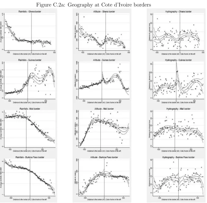
We then check for the absence of discontinuities in predetermined variables, in keeping with the spirit of the tests for observational comparability of treatment and control groups in randomized designs. Three geographical variables are exam-ined: rainfalls (average millimeters per day over the 1984-2001 period), altitude (in meters above the sea level), and hydrography (distance in kilometers to the closest river within the hydrological basin). We additionally look at latitude for North-South oriented borders and at longitude for West-East borders; in the case of the borders of Guinea with Cote d’Ivoire and Mali, and of Burkina Faso with Mali, we look at both.
We last test for the continuity in ethnic composition, using the shares of two broad ethnic groupings: the Akan at the Cote d’Ivoire/Ghana border and the Mande-Voltaic at the three other borders. The locally linear estimator described in equation (2) shows that we can most often reject with confidence the existence of border discontinuities in geography or ethnic composition, for all bandwidths between 50 km and 150 km in four cases out of eight, or at least for the optimal
bandwidth hoptCV that we selected in two additional cases (Cote d’Ivoire with Ghana
and Burkina Faso).15 The two exceptions that arise are the borders of Guinea.
At the border with Cote d’Ivoire a discontinuity is observed for rainfalls, altitude and hydrography: the Guinea side is 200 meters more elevated, further away from rivers, and receives a rain supplement of 3.7 millimeters per day. At the border of Mali, the Guinea side appears 180 meters lower in altitude and more distant to rivers by 10 kilometers, however no difference in rainfalls is observed. We conclude that the comparisons at Guinea borders can be questionable because of boundaries following terrain discontinuities and rivers, as our research concerning the alignment of boundaries indeed confirms (see appendix A).
We now turn to border discontinuities in development outcome variables. We first focus on cash expenditures per capita because this variable constitutes the most obvious welfare indicator. Total consumption expenditures, i.e. including
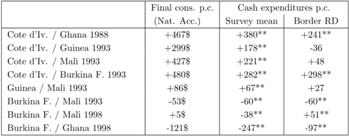
consumption of own food production, is more dependent on differences between surveys and on pricing choices, and is not available for Mali 1994. Results obtained for this latter variable are however consistent with those obtained with the former. We also look at the non-food expenditures share (the denominator being here total consumption). The first column of figure 6 features the results of equation (2) esti-mation of discontinuities in cash expenditures per capita at the four Cote d’Ivoire borders and for the whole span of bandwidths ranging from 50 km to 150 km; the second column presents the results of equation (3) placebo border discontinuities. Figure 7 provides the same for the four borders between Cote d’Ivoire neighbors. Table 2 gathers the results obtained at optimal bandwidths whose determination was explained in section 3 above, and which are indicated by vertical lines in the first columns of figures 6 and 7; the RD estimates are compared with differences in final consumption expenditures per capita from national accounts and with differences in national means of cash expenditures per capita from the surveys.
[ Insert Figure 6 about here ]
Two large discontinuities are revealed at the borders of Cote d’Ivoire with Ghana and Burkina Faso, while at the borders with Guinea and Mali results convey a much more ambiguous conclusion.
In the case of Ghana, a jump of around 200 dollars (at 1988 prices and dollar) is observed with bandwidths ranging between 50 km and 95 km, as well as with wider ones above 145 km (see top left graph of figure 6). For bandwidths ranging between 100 km and 140 km, the inclusion of Abidjan, the capital city of Cote d’Ivoire, into the estimation sample results in a steep downward slope to the border and in a spurious cancelation of the border effect. At the selected bandwidth of 80 km, the discontinuity reaches 241 dollars, compared to 341 dollars for the national means difference, and 467 dollars for national accounts final consumption (table 2); bandwidths larger than 140 km also point to the same magnitude. Hence, as with border districts comparisons in means (see above section 4), some attenuation
occurs at the border, but we still find a very significant contrast in income when crossing the border. Placebo regressions show that this 241$ discontinuity no longer holds as soon as the border line is shifted by more than 25 kilometers on either side (figure 6, top right graph). On the Cote d’Ivoire side (right part of the graph), the placebo discontinuities that arise at higher distances, a negative one at around 35 kilometers followed by a positive one around 80 kilometers, are due to the already mentioned Abidjan perturbation.
In the case of Burkina Faso, almost all bandwidths point to a discontinuity ranging between 200 and almost 300 dollars (figure 6, left graph of second row), the maximum of 298 dollars being reached at the optimal bandwidth of 135 km (table 2), here with no attenuation with regard to the national means difference. Here again, the placebo RDs are very neat and confirm that the discontinuity
indeed lies at the border and not elsewhere.16
[ Insert Table 2 about here ]
Conversely, Guinea and Mali figures only exhibit significant discontinuities for bandwidths lower than 75 km that we cannot entirely rely upon. Indeed, at optimal bandwidths of respectively 130 and 120 kilometers, the estimated border treatment effects are small in magnitude and insignificant. In the case of the Guinea border, the result fits with the negative and insignificant district-level mean differences already observed in section 4. We should also recall that it could uncover geographical discontinuities that make its interpretation difficult. In the 16In relative terms, that is when divided by the estimate at D = 0 for the corresponding
comparison country, these numbers mean respectively a doubling of cash expenditures when crossing the Ghana border toward Cote d’Ivoire, and a tripling at the Burkina Faso border. Very similar figures are obtained when taking total consumption instead of cash expenditures. When looking at non-food expenditures share, in the case of Ghana a significant discontinuity of more than 7.5 percentage points is only observed with bandwidths over 140 km, while in the case of Burkina Faso a large discontinuity ranging between 10 and 20 percentage points is observed at almost all bandwidths.
case of the Mali border, the outcome varies with distance to the border on the Cote d’Ivoire side, cash expenditures being lower for households who live closer to the border. This explains why the RD estimate is not the same as from district-level mean differences. All we can say is that the discontinuity lies between 0 and 100 dollars, and as such is much lower than the one observed at the Burkina Faso border, despite the fact that the two northern countries have rather close national incomes (table 2).
These discontinuities in cash expenditures at Cote d’Ivoire borders are strik-ingly consistent with the discontinuities prevailing at borders between Cote d’Ivoire neighbors, that are displayed in figure 7 and in the bottom part of table 2. The border between Guinea and Mali again provides an ambiguous figure: no discon-tinuity at all when taking bandwidths from 50 to 110 km, the optimal bandwidth being set at 75 km; or some Guinean advantage between 100 and 150 dollars with bandwidths ranging from 110 to 150 km. Among the triangle formed by border areas between Cote d’Ivoire, Guinea and Mali, we cannot definitely reject the wel-fare ranking Cote d’Ivoire > Guinea > Mali that corresponds to national accounts or national samples figures. However, we cannot reject either the assumption of an homogenous space. And at optimal bandwidths, border discontinuities rather tell that Cote d’Ivoire = Guinea = Mali, or at least that discontinuities in income are too small to be identified. And geographical discontinuities that were spotted above come to blur the picture even more.
[ Insert Figure 7 about here ]
Conversely, among the triangle formed by border areas between Cote d’Ivoire, Burkina Faso and Ghana, the welfare ranking is clearer, even if discontinuities are evaluated at different periods: Cote d’Ivoire > Ghana > Burkina Faso. Indeed, the last graph of figure 7 and the last row of table 2 show that an unambiguous discontinuity holds at the border between Ghana and Burkina Faso in 1998, with a 50$ or so advantage for Ghana (at 1998 prices and dollar exchange rates). The
border discontinuities are pretty much consistent with Cote d’Ivoire remaining wealthier than Ghana even in 1993 or 1998, in spite of some convergence since 1988, but with Ghana standing in between Cote d’Ivoire and Burkina Faso, as reflected by official national accounts data and border districts comparisons mentioned in section 4.
Between Mali and Burkina Faso, it is striking that at optimal bandwidths there is a small Malian advantage of 60$ around the years 1993-94, then followed by a Burkina Faso advantage of 51$ in the years 1998-2001. The latter figure of switched positions is less robust than the first in terms of bandwidth variation, but we can tell that the border discontinuity most probably lies between 0 and 50$ in 1998-2001. Anyway, the two figures are rather consistent with the evolution of national accounts and national samples contrasts that reveal a melting down of the Malian income advantage. Like in the 1986-1998 evolution analyzed in section 4 figure 3 at the Cote d’Ivoire/Ghana border, this is revealing of the insulating power of borders that help in preserving countries from the macroeconomic ups and downs of neighbors. Indeed, 2001 is a bad year for Mali as it corresponds to a long-lasting strike of cotton producers who are located in the southern part of the country, i.e. near the borders with Cote d’Ivoire and Burkina Faso. Last, if we stick to the 1993-94 figure, we preserve the following transitive ranking Cote d’Ivoire ≥ Mali > Burkina Faso.
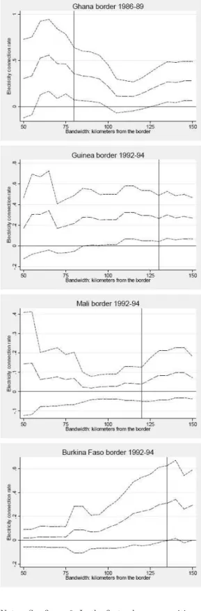
Figure 8 displays RDs estimates and Placebo RDs for connection to electric-ity. With this variable, inference is more difficult due to spatial auto-correlation. However, the Cote d’Ivoire advantage is fairly robust at the borders with Ghana and Guinea: in both cases, the border RD is estimated between 15 and 50 percent-age points of connected individuals. It is also salient at the Burkina Faso border, and using the optimal bandwidth delivers the same order of magnitude i.e. around 30 percentage points, although the RD coefficients are less robust to bandwidth variation. Conversely, the Cote d’Ivoire advantage is definitely canceled out at the borders with Mali. In the case of Mali, the 25 percentage points difference provided
by district-level analysis gets down to an insignificant 5 points difference with the 120 kilometers optimal bandwidth. Like with the consumption comparisons exam-ined above, the lack of precision and arbitrariness of the administrative grid can explain the bias of district-level means comparisons: in particular, the southern part of Cote d’Ivoire border districts includes larger cities (Odienne, Boundiali, Korhogo) that are well-connected, whereas villages located near the border are
not.17
[ Insert Figure 8 about here ]
Turning back to the case of Guinea, the connection to electricity figure seems to contradict the absence of discontinuity in terms of living standards, and to be revealing of a difference between the determinants of public investment and of private income; however, the geographical discontinuities that were spotted at this border could also explain why more mountainous areas on the Guinea side have less chances to be connected. Still, no discontinuity in connection to electricity is observed at all the other borders between Cote d’Ivoire neighbors (results not shown), even if the coastal countries, Ghana and Guinea, display much higher national rates (respectively 27 and 20% in 1992-94) than landlocked countries, Mali and Burkina Faso (both 5% only). This allows to consider that it is truly the higher public investment effort of wealthier Cote d’Ivoire that translated into peripheral areas, the border with Mali standing as an exception.
We last look at discontinuities in adult literacy, to be compared with na-tional and district-level differences depicted in figure 4 shown above. For the sake of space we only summarize the results here. RD estimates are broadly in line 17Access to safe water other than rainfall and rivers (wells, taps, etc.) also jumps at the borders
of Cote d’Ivoire with Ghana (by more than 20 percentage points) and with Burkina Faso (by more than 35 points) at optimal bandwidths. No discontinuities are found at the borders with Guinea and with Mali. In the case of Guinea however, the hydrographic discontinuity already spotted, with Guinean localities being further away from rivers, precludes an unambiguous conclusion.
with border residents mean differences of figure 4. Recall that we cannot correct here for migration, as distance to the border is not available for internal migrants (only district of birth is recorded, not precise place of birth). As already seen, this generates a little attenuation bias of the Cote d’Ivoire advantage. For men born between 1930 and 1959 a large discontinuity is observed at the advantage of Ghana against Cote d’Ivoire (more than 20 percentage points), but thanks to Cote d’Ivoire catching up, this advantage is canceled out for men born after 1960. No discontinuity in adult literacy is observed between border residents of the four former French colonies for people born before 1960, i.e. before national boundaries came into being. Conversely, for people born after independence, some disconti-nuities are observed at optimal bandwidths: at the border of Cote d’Ivoire with Guinea for women (around 20 percentage points), and at the border with Burkina Faso for both men and women (20 points again). In this latter case, district-level mean comparisons of figure 4 reveal more blurred than RDs; consistently enough, between Ghana and Burkina Faso a significant RD of around 20 points is observed for both men and women born after 1960, at the advantage of the former country. Finally and again, the border of Cote d’Ivoire with Mali provides a more ambigu-ous picture, as we detect no significant RD whether in adult literacy or in past school attendance (ever been at school), in contrast with what figure 4 suggested. To summarize, the advantage of being included in one of the two wealthiest countries, first Cote d’Ivoire and second Ghana, is still fairly visible very far from the capital cities Abidjan and Accra and from the coast, in the northeastern area around Burkina Faso, where we spot large discontinuities prevailing in terms of monetary welfare, connection to electricity or access to water, and adult literacy. In the northwestern part around Guinea and Mali, the existence of border dis-continuities is much less obvious, depending sometimes on the bandwidth that is chosen, the less ambiguous case being electricity connection at the Cote d’Ivoire / Guinea border. This northwestern part, and in particular the border with Mali, is precisely the furthest away from the capital city of Cote d’Ivoire, Abidjan, so that
Herbst’s model of radiating core finds here an illustration. However, when look-ing at borders which divide countries with closer levels of development and whose distance to both capital cities is broadly the same, like between Cote d’Ivoire and Ghana on the one hand, or Burkina Faso and Mali on the other hand, signifi-cant discontinuities are also observed, even if of smaller magnitude. The size and the sign of these discontinuities are determined by the ups and downs of the na-tional macroeconomic climates, which is revealing again of the insulating power of national borders.
6
Conclusion: Borders matter
In Africa, boundaries delineated during the colonial era now divide young independent states. The borders between Cote d’Ivoire and four of its neigh-bors (Ghana, Guinea, Mali and Burkina Faso) separate fairly comparable areas in terms of geography, anthropology and pre-colonial history. Nevertheless, by ap-plying regression discontinuity designs to a large set of household surveys covering the 1986-2001 period, this paper identifies many large and significant jumps in welfare at borders. Border discontinuities mirror the differences between country averages with respect to household income, public investment and education, and are revealing of the centripetal forces of national markets and public investment policies. Taking into account migration flows does not change this diagnosis, as
they are rather part of the story.18 However, distance to the capital city has a
strong power of attenuation, so that border discontinuities are blurred or even erased in the most remote peripheral areas. These results are very consistent with a national integration process that is underway but not yet achieved. National borders already matter in Africa, and the country of residence makes a difference.
18As shown, intense and selective migration flows run from peripheral areas to the centers, but
international migrants from poor landlocked countries also find beneficial to settle just on the other side of the border next to their country of origin.
Figure 1: Cash exp enditures p er capita: National and b order lev els around 1993 Reading: The map distinguishes the administrativ e b order districts means and the rest of the coun try means. In the case of the b orders with Mali and Burkina F aso, the F erk essedougou district is included in b oth b order means on the Cote d’Iv oire side (see also app endix A, figure A.1). Unit: 1993 prices and 1993 dollars.
Figure 2: Connection to electricit y: National and b order lev els around 1993 Reading: The map distinguishes the administrativ e b order districts means and the rest of the coun try means. In the case of the b orders with Mali and with Burkina F aso, the F erk essedougou district is included in b oth b order means on the Cote d’Iv oire side (see also app endix A, figure A.1).
Figure 3: Living standards across time at Ghana border
Coverage: Households (weighted by household size and sample weights).
Reading: National means computed from surveys are in solid line, border means (along with upper and lower bounds of 95% confidence intervals) are in dashed lines. In the first graph, national accounts private consumption per capita is added (top line, long dash). Errors are clustered by PSUs.
Figure 4: Literacy at Cote d’Ivoire borders
Coverage: Individuals born 1930-1980 (1974 for Ghana comparison).
Note: OLS fits of quartics in date of birth. National (solid line): Country natives (Cote d’Ivoire, Ghana and Guinea) or country residents (Mali and Burkina Faso). Border natives line (long dash): For Ghana and Guinea borders, only internal migrants on both sides. For Mali and Burkina Faso, internal migrants from border areas only on the Cote d’Ivoire side; nationals from Mali and Burkina Faso in Cote d’Ivoire surveys are included in
Figure 5: Map of b order clusters (100 kilometers band) # # # # # ## # # # # # # # # ## # # # # # # # ## # # # # # # # # # ### # ## ## # # # ### # ####### # # ## ###### ### ##### ### ###### ##### # ## # ### # # # # # # # # ### # # # # ### # # # # ### # # # ## # # # # # ## # # ## # # # # # # ### #### # # ### #### # # ### ### # # ####### # # ##### # # #### # # # # # # ### # # # ### # # # ### # # # # # # ## # # # # # # ## # # # # # # ## # # # # # # # # # # # # # # # # # # # # # # # # # # # # # # ########## # # # # ###### # # # # ##### # # # # # # # ## # # # ## # # # ## # # # # # # # # # # # # # # # # # ## # # ## # # # ## # # # # # # ### # # # # # # # # # # # ## # # # # # # # ######## ### # # # # ######## ### # # # # # # # # # ## # # # ######## ### # # # # # # ## # ## # # # # # # # # # # # # # # # # # # # # # # # # # # # # # # # # # # # # # # # # # # # # # # # # ## ## ### # # # # # # ### # # # # # ## # # # # # ## # # # # # ## # # # # ######### # # # # # ## ## # ### ############### # # ## # # # # # # # # # # # # # # # # # # # # ## ##### # # # # # # # # # # # # # # # # # # # # # # # # # # # # # # # # # # # # # # # # # # # # # # # # # # # ## A tla n tic O c e a n B u rk in a F a s o C ô te d 'Iv o ir e G u in e a M a li G h a n a L ib e ri a Reading: Eac h dot corresp onds to a PSU not further aw ay than 100 kilometers from the b order. A t the Cote d’Iv oire / Ghana b order, only surv ey clusters for the 1986-1989 p erio d are plotted; at the three other b orders, only surv ey clusters for 1992-1994 are plotted.
Figure 6: Cash expenditures per capita: Discontinuities at Cote d’Ivoire borders
1st column: RDs at borders estimated by locally linear regressions with variable bandwidths, see equation (2) in the text. The estimated coefficient of the Cote d’Ivoire dummy γ(h) is plotted against bandwidth h, with a 95% confidence interval band. Vertical lines indicate optimal bandwidths hoptCV (cross-validation criterion, see text). 2nd column: Placebo RDs, see equation (3) in the text. Bandwidths hoptCV are those indicated in the 1st column. The estimated coefficient for the discontinuity γ(k) at a fictional border (cutoff) shifted from the actual border by k kilometers, is plotted against k, with a 95% confidence interval band.
Figure 7: Cash expenditures per capita: Discontinuities at borders between Cote d’Ivoire neighbors
Notes: See figure 6. In the first column, a positive number indicates a welfare advantage for the first country
Figure 8: Connection to electricity: Discontinuities at Cote d’Ivoire borders
Table 1: Surveys
Neighbor survey Cote d’Iv. survey Period Sample size (# households) Comparison
country
Cote d’Ivoire Comparison country
Cote d’Ivoire Ghana GLSS1-2 CILSS2-4
Feb.86-May.89
Mar.87-Apr.89
6,336 4,814
Ghana GLSS3 ENV1
Sep.91-Sep.92
Apr.92-Oct.93
4,558 9,598
Ghana GLSS4 ENV2
Apr.98-Mar.99
Sep.98-Dec.98
6,016 4,178
Guinea EIBC ENV1
Jan.94-Feb.95
Apr.92-Oct.93
4,417 9,598
Mali EMCES ENV1
Mar.94-June94
Apr.92-Oct.93
9,554 9,598
Mali EMEP ENV2
Jan.01-Jan.02
Sep.98-Dec.98
7,365 4,178 Burkina Faso EP1 ENV1
Oct.94-Jan.95
Apr.92-Oct.93
8,642 9,598 Burkina Faso EP2 ENV2
May98-Aug.98
Sep.98-Dec.98
8,469 4,178
Note: The three first Ivorian (CILSS 2 to 4) and the two first Ghanaian (GLSS 1 and 2) surveys are stacked in order to obtain large samples covering the 1986-89 period.