FIERAsystem: A Fire Risk Assessment Model for Light Industrial Building Fire Safety Evaluation

(1)

Publisher’s version / Version de l'éditeur:

Vous avez des questions? Nous pouvons vous aider. Pour communiquer directement avec un auteur, consultez la

première page de la revue dans laquelle son article a été publié afin de trouver ses coordonnées. Si vous n’arrivez

Questions? Contact the NRC Publications Archive team at

PublicationsArchive-ArchivesPublications@nrc-cnrc.gc.ca. If you wish to email the authors directly, please see the first page of the publication for their contact information.

https://publications-cnrc.canada.ca/fra/droits

L’accès à ce site Web et l’utilisation de son contenu sont assujettis aux conditions présentées dans le site LISEZ CES CONDITIONS ATTENTIVEMENT AVANT D’UTILISER CE SITE WEB.

Research Report (National Research Council of Canada. Institute for Research in

Construction), 2002-11-01

READ THESE TERMS AND CONDITIONS CAREFULLY BEFORE USING THIS WEBSITE.

https://nrc-publications.canada.ca/eng/copyright

NRC Publications Archive Record / Notice des Archives des publications du CNRC : https://nrc-publications.canada.ca/eng/view/object/?id=52857fa6-fdd5-4fc6-b74e-0b73a18cee30 https://publications-cnrc.canada.ca/fra/voir/objet/?id=52857fa6-fdd5-4fc6-b74e-0b73a18cee30

NRC Publications Archive

Archives des publications du CNRC

For the publisher’s version, please access the DOI link below./ Pour consulter la version de l’éditeur, utilisez le lien DOI ci-dessous.

https://doi.org/10.4224/20378844

Access and use of this website and the material on it are subject to the Terms and Conditions set forth at

FIERAsystem: A Fire Risk Assessment Model for Light Industrial

Building Fire Safety Evaluation

(2)

FIERAsystem: A Fire Risk Assessment Model for Light Industrial

Building Fire Safety Evaluation

Bénichou, N.; Kashef, A.; Torvi, D.;

Hadjisophocleous, G.; Reid, I.

IRC-RR-120

November 2002

(3)

FIERAsystem: A Fire Risk Assessment Model for Light Industrial

Building Fire Safety Evaluation

Noureddine Benichou, Ahmed Kashef, David Torvi, George Hadjisophocleous, and Irene Reid

Research Report #120

November 2002

Fire Risk Management Program Institute for Research in Construction National Research Council Canada

(4)

List of Figures

FIGURE 1 SIMPLE CORRELATION COMPONENTS... 3

FIGURE 2 MODIFICATION OF HEAT RELEASE RATE USING SUPPRESSION EFFECTIVENESS VALUE, η... 9

FIGURE 3 QUANTITIES USED TO CALCULATE FIRE DEPARTMENT RESPONSE AND INTERVENTION TIME... 11

FIGURE 4 EXAMPLE OF FIRE SPREAD IN A MULTI-COMPARTMENT BUILDING... 18

FIGURE 5 PROCEDURE FOR FIERASYSTEM HAZARD ANALYSIS... 19

FIGURE 6 HAZARD ANALYSIS SUMMARY... 20

FIGURE 7 FIERASYSTEM FIRE RISK ASSESSMENT PROCESS... 21

List of Tables

TABLE 1 PROCEDURE FOR FIERASYSTEM HAZARD ANALYSIS... 17

(5)

Nomenclature

A area (m2)

CO concentration of carbon monoxide (ppm)

D diameter (m)

E emissive power (kW/m2) END expected number of deaths

F radiation view factor (dimensionless)

f fraction of heat release rate that is considered radiative (dimensionless) FID fractional incapacitating dose (dimensionless)

g acceleration due to gravity (m/s2)

H height (m)

k factor to account for effect of compartment walls (dimensionless) P probability (dimensionless)

POP population

Q heat release rate (kW) q" heat flux (kW/m2)

r distance (m)

S experimental parameter (m-1) SF safety factor (dimensionless) T temperature (°C, K)

t time (s)

V thermal dose ((kW/m2)4/3·s)

ν burning rate (m/s)

VCO2 multiplication factor for CO2-induced hyperventilation (dimensionless)

Y probit function (dimensionless)

%CO2 concentration of carbon dioxide (percentage)

Greek Letters

a fire growth coefficient (kW/s2)

η suppression effectiveness value (dimensionless)

τ atmospheric transmissivity

ξ dummy variable for integration

Subscripts

act at time of activation

amb ambient C compartment ce ceiling impingement CO carbon monoxide D death e emissive ep effective plume f fire, flame HG hot gases i index m modified max maximum resid residual S hot gas layer

s smoke

TG toxic gases

TR thermal radiation

(6)

1. INTRODUCTION

As Canada and other countries move from prescriptive-based building codes to performance/objective-based codes, new design tools are needed to aid in demonstrating that compliance with these new codes has been achieved. One such tool is the computer model FiRECAM™, which has been developed over the past decade by the Fire Risk

Management Program of the Institute for Research in Construction at the National Research Council of Canada (NRC). FiRECAM™ is a computer model for evaluating fire protection systems in residential and office buildings that can be used to compare the expected safety and cost of candidate fire protection options.

To evaluate fire protection systems in light industrial buildings, a new computer model is being developed. This model, whose current focus is aircraft hangars and warehouses, is based on a framework that allows designers to establish objectives, select fire scenarios that may occur in the building and evaluate the impact of each of the selected scenarios on life safety, property protection and business interruption. This model will assist engineers and building officials in evaluating, in a clear and concise manner, whether a selected design satisfies the established objectives for a building. The new computer model is called FIERAsystem, which stands for Fire Evaluation and Risk Assessment system.

FIERAsystem uses time-dependent deterministic and probabilistic models to evaluate the impact of selected fire scenarios on life, property and business interruption. The main FIERAsystem submodels calculate fire development, smoke movement through a building, time of failure of building elements, and occupant response and evacuation. In addition, there are submodels dealing with the effectiveness of fire suppression systems and the response of fire departments.

FIERAsystem has been designed as a tool that can be used to do a performance-based fire protection engineering design. It is intended to be used by a wide variety of individuals, including fire protection engineers, building officials, fire service personnel and researchers. Although FIERAsystem has a user-friendly interface, the system is intended to be used by qualified individuals, who receive appropriate training in the use of the software. The individual models included in the overall system are based on accepted fire protection engineering practice and were chosen to give an appropriate level of sophistication, and still result in a system that could be efficiently run on a desktop personal computer. This would allow use of the system by all of the intended parties, and facilitate the examination of multiple fire scenarios and fire protection engineering options. It is the selection of the individual models to be included in FIERAsystem, and the development of the process by which the individual models were combined into the overall system model, which provided the main challenge to the team that developed FIERAsystem. The individual models chosen and the overall system model are described in subsequent sections in this report.

The current report describes the framework for the new model, individual submodels used for calculations, and the information that the model provides to the design engineer or building official. The framework that FIERAsystem uses to conduct a hazard analysis and the process used to perform a risk analysis are also discussed in the report.

(7)

2. FRAMEWORK OF FIERAsystem MODEL

The FIERAsystem model allows the user to perform a number of fire protection engineering calculations in order to evaluate fire protection systems in industrial buildings. At start-up, FIERAsystem provides several calculation options, which allow the user to: Ø use standard engineering correlations,

Ø run individual submodels, Ø conduct a hazard analysis, or Ø conduct a risk analysis. 2.1 Simple correlations

The standard engineering correlations model (FIERAscor) is a collection of relatively simple equations and models that can be used to quickly perform simple fire protection engineering calculations. The current version of FIERAscor contains procedures for calculations in the general areas of fire development, plume dynamics, smoke movement, egress, fire severity and ignition of adjacent objects. A more complete listing of the

correlations that are included in FIERAscor is given in Figure 1. 2.2 Individual submodels

Individual submodels in FIERAsystem can be used to evaluate single components of a fire safety design, such as the time of activation of heat detectors or sprinklers, the time to flashover and the time of failure of construction elements. This allows the user to calculate the quantities of interest to them, without having to do a complete FIERAsystem analysis. Each individual model has its own user interface and is designed as a stand-alone piece of software. The user, therefore, only has to enter the input data required by that particular model, rather than having to enter all of the information required by all of the models in the complete system.

It should also be noted that FIERAsystem could be used to evaluate whether a fire protection system for a building will satisfy specific fire safety objectives. This can be done using individual submodels, or through a hazard or risk analysis. An example of the use of FIERAsystem in evaluating compliance with fire safety objectives can be found in Reference [2].

The individual submodels included in FIERAsystem are described in the next section.

2.3 System flexibility

FIERAsystem provides flexibility in performing fire protection engineering

calculations. The system model has been set up so that a calculation can be performed to evaluate a single part of the fire protection system by running only a single submodel, such as the detection model. A complete hazard or risk analysis can also be conducted using the models supplied with FIERAsystem. Alternatively, this hazard or risk analysis can be

performed using a combination of some of the FIERAsystem models and information from datafiles. Recognizing that in many cases, fire protection engineers must still rely on empirical data, where models have not yet been developed, these datafiles can include fire

(8)

test data. Datafiles containing results from other computer fire models can also be used. This flexibility allows FIERAsystem to be used by designers of many different types of buildings, since modifications can be made to individual submodels, without having to change the rest of the system model.

Figure 1 Simple correlation components

FIERAscor

Fire Development Plume Smoke Others

Egress Time

Fire Severity

Radiant Ignition of Adjacent Fuel Heat Release Rate for a

t² Fire

Heat Release Rate for a Pool Fire

Heat Release Rate for a Fully Developed Fire

Heat Release Rate of Decay Thomas Flashover Correlation McCaffrey Flashover Correlation Flame Height

Lateral Flame Spread

Plume centerline Temperature

Entrained Mass Flow Rate Average Plume

Temperature

Plume Filling Rate

Plume Gas Density

Plume Rise

Plume Diameter

Compartment Temperature during

Pre-Flashover

Volume Rate of Smoke

Smoke Filling

Atrium Temperature Rise

Ceiling Jet Temperature Compartment Temperature during

(9)

3. FIERAsystem SUBMODELS

In FIERAsystem, various models are used to make the necessary calculations to evaluate candidate fire protection systems. Each model can be run independently, or in conjunction with other models to perform a complete risk or hazard analysis. The main FIERAsystem submodels are described briefly in this section. More detailed information on each of these submodels can be found in separate publications (e.g., [3,4]).

3.1 Fire Development

Models are currently available in FIERAsystem for the following fire scenarios: Ø liquid pool fires,

Ø storage rack fires, and

Ø t2 fires (i.e., the heat release rate is assumed to be proportional to the square of the elapsed time, which is often used to simulate fires).

Each of the Fire Development Models calculates the quantities that characterize the fire (heat release rate, temperature and thermal radiation heat fluxes) as functions of time. Currently, the equations used are standard engineering correlations, such as those found in the SFPE Handbook of Fire Protection Engineering [5]. For example, a confined, enclosed pool fire was chosen as one of the fire scenarios in the case studies, described in

Appendix A. The heat release rate at any time, Q(t), is calculated by assuming that the pool fire can be described as an ultra-fast t2 fire, using the following equation [6]:

2

t a

Q(t)= Eq. 1

Where:

Q = the heat release rate of the fire at any time (kW), and α = the fire growth coefficient (kW/s2)

= 0.1876 kW/s2.

This heat release rate is limited to the maximum heat release rate possible based on either the amount of fuel in the compartment or the oxygen that can be supplied to the fire from the compartment and through ventilation openings.

The duration of a confined pool fire is calculated using the volume of fuel burned, the dike area and the burning rate of the fuel, which are specified by the user. The model assumes that the diameter of a confined pool fire increases linearly with time from 0.3 m to the maximum diameter, Dmax, entered by the user. The assumption that the initial diameter

of the fire is 0.3 m is based on calculating the diameter for which a heat flux of 140 kW/m2 is predicted using a simple point source representation of a 100 kW fire size with 40% of the heat release rate assumed to be radiative. While the point source model generally under-predicts heat fluxes relatively close to a fire, it still provides a simple method of ensuring that the nominal diameter is realistic for the particular fire being modelled. A 100 kW fire is about the size of a fire in a small wastepaper basket. This is thought to be a good estimate of the initial size of any fire that would be of interest to the engineers using FIERAsystem.

(10)

The assumption that the diameter increases linearly with time is based on the fact that the maximum fuel-controlled heat release rate of a fire is a function of the area of the fire, which is a function of the square of the diameter of the fire. Therefore, as a t2_fire

assumes that the heat release rate is a function of the square of the elapsed time, it follows that the diameter will be a linear function of time for a t2 fire. The time required to reach this maximum diameter, tmax, is given by the following equation [7]:

(

)

1/3 max f max max D gv D 564 . 0 t = Eq. 2 Where:

νf = the burning rate of the fuel (m/s), and

g = the acceleration due to gravity (m/s2).

The thermal radiation heat fluxes from the pool fire to a point on a plan located 1 m above the ground are calculated using the solid flame model of Mudan and Croce [7]. The current two-zone model assumes that the visible portion of the flame emits a relatively high amount of thermal radiation, while the non-visible gases do not emit a significant amount of thermal radiation. The following equation is used to calculate thermal radiation heat fluxes at a distance, q′′(t), from the fire:

SF ) t ( F " q ) t ( " q = e τ Eq. 3 Where:

q"e = the emissive power of the pool fire (kW/m2);

F(t) = the view factor from the pool fire to the point, calculated using the height and diameter of the flame (0 ≤ F ≤ 1);

τ = atmospheric transmissivity (assumed to be 1.0, because of the relatively short distances considered); and

SF = a safety factor (default value = 1).

A height of 1 m was chosen so as to be representative of the mid-section of a

person. The lower, high-emitting portion of the fire is assumed to have an emissive power of 140 kW/m2, while the upper, low-emitting portion is assumed to have an emissive power of 20 kW/m2. The emissive power of the flame, q"e, is then calculated using the following

equation: ) e 1 ( E e E " q SD s SD f e = − + − − Eq. 4 Where:

Ef = the maximum emissive power of the visible portions of the fire (kW/m2),

= 140 kW/m2

Es = the maximum emissive power of the smoky portions of the fire (kW/m2),

= 20 kW/m2

D = diameter (m)

(11)

= 0.12 m-1.

Equation 4 was developed to estimate the average emissive power of large, sooty hydrocarbon fires using experimental data reported in the literature.

At each time step, the heat flux from the pool fire is calculated at the outside of each of a number of rings located from the center of the room to the boundary of the

compartment. These heat fluxes are used by the Life Hazard model to calculate the probability of death from exposure to high heat fluxes.

The Fire Development Model supplies the Building Element Failure Model, which is described later, with information to calculate the convective and radiative heat fluxes from the fire to the boundaries of the compartment. First the temperature at the centreline of the visible portion of the flame (Tf) is assumed to be 980°C and the emissivity of the fire is

assumed to be 1.0. This temperature and emissivity correspond to the thermal radiation heat flux of 140 kW/m2 assumed earlier for the visible portion of the flame. The ceiling impingement temperature (Tc) at any time is calculated using the following equation [8]:

5/3 c H 2/3 (kQ(t)) 0.22 amb T (t) c T = + Eq. 5 Where:

Tamb = the ambient temperature (°C);

k = a factor to take into account the effect of the compartment walls on the

temperature of the hot plume gases;

= 1 (if no walls are nearby);

= 2 (if the fire is close to one wall – default value); = 4 (if the fire is in a corner); and

Hc = the compartment height (m).

Alpert and Ward [8] stated that Equation 5 was derived from empirical data and was not valid when the flames are either very close to the ceiling or very far away from the ceiling; therefore, it cannot predict temperatures greater than 825°C accurately. Therefore, if the temperature predicted by Equation 5 is greater than the 980°C temperature assumed for the flames, the model limits the ceiling impingement temperature to 980°C.

While the heat transfer to the ceiling of a compartment can be calculated using the ceiling impingement temperature, an effective plume temperature based on the flame and ceiling impingement temperatures is calculated in order to determine time to failure of the walls of the compartment. This is because of the fact that the FIERAsystem Building Element Failure Model uses only a single temperature to represent the effects of the fire on the walls (e.g., the hot gas temperature in a fire resistant test furnace). Therefore, the FIERAsystem Fire Development Model calculates an effective plume temperature (Tep) to

account for heat transfer from both the visible flame and the hot gases in the fire plume above the visible flame to the walls. This effective plume temperature is calculated based on a simple model of the thermal radiation heat transfer from the flame and hot gases. The view factors from the flame and hot gases are assumed to be proportional to their surface areas, and hence their heights. The initial wall temperature is assumed to be close to

(12)

ambient. All emissivities are assumed to be one, and only thermal radiation heat transfer between the walls and the flame and hot gases are considered. The total thermal radiation heat flux from the flames and hot gases is then equated with the thermal radiation heat flux calculated using a single effective plume temperature, Tep4(t):

(t) T H (t) H 1 (t) T H (t) H ₄ ce c f 4 f c f     − + = (t) T_ep4 Eq. 6 Where:

Hf(t) = the height of the flame (m),

Hc = the height of the compartment (m),

Tce(t) = ceiling impingement temperature (K),

Tf(t) = flame temperature (K), and

Tep(t) = effective plume temperature (K).

3.2 Smoke Production and Movement

FIERAsmoke is a two-zone model developed at NRC for calculating smoke

production and spread through the compartments in a building. For each of the two zones, differential equations based on mass, energy and species conservation are solved, subject to boundary and initial conditions based on user input. These equations consider the combustion process, vent flows, plume entrainment, and conduction, convection and

radiation heat transfer. The output of this submodel provides information on the temperature and thickness of smoke layers and species concentrations throughout the building. Thermal radiation heat fluxes from the smoke layer in each compartment are also calculated by the model. More details on this model can be found in Fu and Hadjisophocleous [3].

3.3 Fire Detection

Activation times of heat detectors, smoke detectors and sprinkler heads are determined using the Fire Detection Model. When the model is run on its own, the user is asked to specify the location of the fire source and the locations and types of any detectors or sprinklers. In an automated hazard analysis, the fire source is assumed to be centered between the detectors and sprinklers, resulting in the largest possible distance from the detectors and sprinklers. The time-dependent heat release rate and effective diameter of the fire source are also input. Standard engineering correlations are used to predict the temperatures and velocities at different locations within the fire plume, ceiling jet and smoke layer [9].

This information is then used to calculate the temperatures of all detection elements in the space with time. The time-dependent temperature of each detection element (or rate of temperature increase, for rate of rise detectors) is then used to determine the activation time of each heat detector and sprinkler head in the space. Information on the smoke layer is used to predict the activation time of smoke detectors in the space. Activation times for detectors and sprinklers are used to help determine the occupant response time and the fire department response time.

(13)

3.4 Building Element Failure

Times to failure for the structural elements and barriers in the building are estimated using the Building Element Failure Model. Presently, the program can perform calculations for steel beams and columns, concrete slabs, wooden beams and columns, and wood-frame walls and floors. The user may choose to conduct the calculations based on standard fire protection engineering correlations, or use numerical techniques, such as finite difference heat transfer models, for some structural elements. The output of these models consists of the predicted time of failure of the structural element or barrier and, in some cases, the yield stress and modulus of elasticity at elevated temperatures. The predicted failure times of the building elements are used by the fire-spread submodel to calculate spread of fire from the compartment of fire origin to other compartments in the building.

3.5 Suppression Effectiveness

The Suppression Effectiveness Model calculates the effect of automatic suppression systems on fires in the building. The model requires the user to input a suppression

effectiveness value (η) from 0 to 1.0, which quantifies the ability of the automatic

suppression devices to extinguish the fire scenarios being considered. This value is then used to modify the fire heat release rate, diameter, thermal radiation heat fluxes and plume temperature. The heat release rate curve, Q(t) (from the Fire Development Model or another source) is input to the Suppression Effectiveness Model. The suppression

effectiveness value is used to produce a modified heat release rate curve, Qm(t) (Figure 2).

It is assumed that if the suppression system effectiveness is 1.0, the fire is controlled so that the heat release rate remains at its value at the time of automatic suppression system activation (i.e., Qm = Qact). This assumption is conservative, as the sprinkler may in fact

extinguish the fire. If the effectiveness is 0, the original heat release rate curve (Qo) will not

be modified (i.e., Qm = Qo). If the effectiveness is between 0 and 1.0, the modified heat

release rate will be calculated at each time step using the following equation:

Qm(t) = (1.0-η)*( Qo(t) – Qact(t) ) + Qact (t) Eq. 7

In the case where heat release rate values decay, any value of Q(t) which is below

Qact is not modified in any way. This helps ensure that the suppression effectiveness model

does not increase the value of Q(t) in this situation.

Heat fluxes and temperatures are then corrected using the modified heat release rate data. If it is assumed that the thermal radiation heat fluxes (q”(t)) at a distance (r) from a fire of heat release rate (Q(t)) can be calculated, assuming a point source model, using the following equation: 2 r 4 ) t ( fQ ) t ( " q π = Eq. 8 Where:

f = the fraction of the total heat release rate that is considered to be radiative. In Equation 8, the thermal radiation heat flux is proportional to Q(t). Therefore, the Suppression Effectiveness Model modifies the thermal radiation heat fluxes using the following equation:

(14)

) t ( q ) t ( Q ) t ( Q ) t ( q " o o m " m = Eq. 9

As the Suppression Effectiveness Model can accept input from fire tests and other models, theory based on the point source method was used. This was thought to be the easiest way to treat heat flux data, even if some models may use a different approach to calculate heat fluxes (e.g., Equation 4).

Figure 2 Modification of heat release rate using suppression effectiveness value, η

In Equation 5, the difference between the ceiling impingement and ambient temperature is proportional to Q2/3. Therefore, the modified ceiling impingement temperature (Tce-o(t)) is determined using the following equation:

3 / 2 o m amb o ce amb m ce ) t ( Q ) t ( Q T ) t ( T T ) t ( T       = − − − − _{Eq. 10}

The ambient temperature, Tamb, in Equation 10 is assumed to be 20°C. The flame

temperature, Tf, is assumed to be 1000°C by the Suppression Effectiveness Model. If an

emissivity of 1.0 is also assumed, this corresponds to a thermal radiation heat flux of approximately 150 kW/m2.

In order to calculate the modified equivalent plume temperature, Equation 6, the original equivalent plume, Tep-o(t), and ceiling impingement temperatures, Tce-o(t), are input to

the Suppression Effectiveness Model for each time step. First, the original ratio of the flame to compartment height is calculated from Equation 6 using the original equivalent and plume temperature and the assumed flame temperature of 1000°C. The Suppression

Effectiveness Model then modifies the ratio of the flame to compartment height. The height of the flames above a fire can be calculated using Heskestad’s correlation [8]:

0 100 200 300 400 500 0 20 40 60 80 100 120 140 160 180 200 H ea tR e lea se R a te (k W ) Time (s) Activation Time = 0.0

η

= 0.5

η

= 1.0

η

(15)

(

)

0.4 f(t) 0.011kQ(t)

H = Eq. 11

Where k was defined previously with Equation 5.

From Equation 11, the flame height is proportional to Q0.4_{. Therefore, the}

Suppression Effectiveness Model modifies the ratio of the flame to compartment height using the following equation:

4 . 0 o m c o f c m f ) t ( Q ) t ( Q H ) t ( H H ) t ( H       = − − _{Eq. 12}

The modified flame to compartment height ratio, Hf - m(t), and ceiling impingement

temperature, Tce-m(t), in Equation 10 are then used along with the assumed flame

temperature of 1000°C to calculate the modified equivalent temperature using the following equation: ) t ( T ) t ( T H ) t ( H 1 ) t ( T H ) t ( H 4 m eq 4 m ce c m f 4 f c m f − − − − ₌     − + Eq. 13

Equivalent temperatures based on the flame and ceiling impingement temperatures are then output to the FIERAsystem Boundary Element Failure Model in order to determine the heat transfer to the boundaries and the time of failure of these boundaries.

3.6 Fire Department Response and Effectiveness

The Fire Department Response Model is used to determine the expected fire

department response and intervention times, which are calculated using the times estimated for notification, dispatch and preparation, travel and set-up (see Figure 3). These

calculations are based on factors such as the fire scenarios selected by the user and activation times for the detectors in the building. The presence of fire alarms in the building (and if they are connected directly to the fire department), occupant response to fire cues or other warning signals, the location of the building relative to the fire department, and

pre-planning, are also considered in the calculations.

Fire starts Fire is reported FD unit is notified FD unit leaves fire house FD unit arrives at scene of fire Unit begins firefighting activities Fire is extinguished Notification Time Dispatch Time Preparation Time Travel Time Firefighting Time Setup Time Response Time Intervention Time Time

(16)

Figure 3 Quantities used to calculate fire department response and intervention time

Once fire department activities begin, the effectiveness of these activities is

estimated by the Fire Department Effectiveness Model according to information on the fire development at the time suppression commences and the resources (e.g., equipment, water and human resources) a available to the fire department. Factors such as the nature of the department (e.g., professional, volunteer or a combination of both), and firefighter

experience and training are also considered in this calculation. 3.7 Occupant Response and Evacuation

The Occupant Response and Evacuation Models are used to track the movement of occupants in the building during the selected fire scenarios, based on the occupant

characteristics entered by the user. Calculations take into account the processes of perception (occupants become aware of fire by means of direct perception of fire cues, warning by alarm or others, etc.), interpretation (occupants make decision to respond), and action (e.g., occupants call fire department, pull alarm, begin to evacuate, etc.). This is different from most occupant evacuation models, which assume that the occupants respond immediately to a fire alarm, or cue, which is not the case in occupant evacuation field studies or real life [10]. Once the occupants respond to the fire, the submodel calculates their movement, taking into account their locations, characteristics, fire development and smoke movement.

3.8 Life Hazard Model

The FIERAsystem Life Hazard Model [4] calculates the time-dependent probability of death for occupants in a compartment due to the effects of being exposed to high heat fluxes and hot and/or toxic gases. The Life Hazard Model uses input from other FIERAsystem models that describe the heat fluxes (Fire Development and Smoke

Movement Models) in the compartment, and the temperature and chemical composition of hot gases (Smoke Movement Model).

The time-dependent probability of death from exposure to high thermal radiation heat fluxes, PTR, at a given location in the compartment, is calculated using the sum of the heat fluxes from the fire (calculated by Fire Development models) and from the hot smoke layer (calculated by the Smoke Movement Model). The revised vulnerability model of Tsao and Perry [11] is used to calculate the probability of death from the heat flux data. This model uses the following probit equation:

V ln 56 . 2 8 . 12 Y = − + Eq. 14 Where:

Y = the probit function, and

V = the thermal dose ((kW/m2)4/3·s).

The thermal dose, V, is calculated using the following equation [12]: ∫ = t 0 3 / 4 dt )) t ( " q ( ) t ( V Eq. 15

(17)

Where:

q" = the incident heat flux (kW/m2_{), and} t = the exposure duration (s)

For a square wave heat flux (i.e., a constant value), Equation 15 reduces to the following equation: t )) t ( " q ( ) t ( V = 4/3⋅ _{Eq. 16}

The probit function, Y, is then used to determine the probability of death due to thermal radiation heat fluxes:

ξ π ξ d e 2 1 ) t ( P 5 Y 2 TR 2 ∫ = − ∞ − − Eq. 17

The probability of death due to breathing toxic gases, PTG, is calculated using the

same techniques originally developed for FiRECAM™ [13]. The FIERAsystem Life Hazard model only considers the toxic effects of CO and CO2, because, in most practical fire

situations, the effects of CO are the most important. CO2 will affect the rate of breathing and

hence will affect the intake of CO. The fractional incapacitating dose due to CO (FIDCO) is

calculated using the following equation and the concentration of CO at a specified height in the compartment of interest:

(

)

_dt 30 ) t ( CO ppm 10 x 2925 . 8 ) t ( FID t 0 036 . 1 4 CO ∫ ⋅ = − Eq. 18 Where:

FIDCO(t) = the fractional incapacitating dose of CO, and

CO(t) = the concentration of CO at time t (ppm)

The FID is defined such that the dose will be lethal when FID = 1. The default height for these calculations is 1.5 m. While it can be argued that all individuals can crawl under a smoke layer at this height, this height was chosen so as to be conservative. The user can also specify other heights for this calculation, depending on the occupancy.

The concentration of CO2 is used to calculate a factor, VCO2, which is used to

increase the FIDCO to incorporate the increase in the breathing rate due to CO2:

(

)

(

)

8 . 6 9086 . 1 ) t ( CO % 2496 . 0 exp ) t ( VCO₂ = ⋅ 2 + Eq. 19 Where:

VCO2(t) = the multiplication factor for CO2 -induced hyperventilation, and %CO2(t) = the percentage of CO2 in the compartment of interest.

(18)

The total fractional incapacitating dose for toxic gases is calculated using the following equation: ) t ( VCO ) t ( FID ) t ( FID_TG = _CO ⋅ ₂ Eq. 20

This FID is then used as the probability of death due to breathing toxic gases (i.e., PTG = FIDTG).

The FIERAsystem Life Hazard model also considers the probability of death due to breathing or being exposed to hot gases, PHG. This probability is equal to the FID for exposure to hot gases, calculated using the following equation [14]:

dt )) t ( T 0273 . 0 1849 . 5 exp( 60 1 ) t ( FID t 0 _S HG ∫ ⋅ − ⋅ = Eq. 21 Where:

TS(t) = the temperature of the hot gases at a height of 1.5 m in the compartment of

interest (°C).

Equation 21 is based on data from the literature for human tolerance times in experimental exposures to dry and humid air at elevated temperatures. A FIDHG of 1.0 is

said to represent the point where a person would become incapacitated by the exposure to the hot gases because of heat stroke, skin burns and/or respiratory tract burns.

The total probability of death, PD(t), at a given location in the compartment is

calculated using the union of the individual probabilities of death from being exposed to high thermal radiation heat fluxes, and breathing hot or toxic gases:

) t ( P ) t ( P ) t ( P ) t ( PD = TR ∪ TG ∪ HG Eq. 22

In order to calculate the total probability of death in any compartment using the FIERAsystem Life Hazard model, the compartment is first divided into a number of rings from the fire, as described earlier in the Fire Development model section. Equation 22 is used to calculate the total probability of death within each of the rings. The total probability of death for the compartment is then calculated using a weighted sum of the probabilities of death in each of the rings:

C i D i i C D A A ) t ( P ) t ( P ∑ = − − Eq. 23 Where:

PD-C(t) = the total probability of death for compartment C,

PD-i(t) = the probability of death for ring i,

Ai = the area contained inside ring i, and

(19)

3.9 Expected Number of Deaths

The expected number of deaths model calculates the number of occupants expected to die in each compartment with time as a result of exposure to toxic and/or hot gases and thermal radiation. This calculation is based on the residual population in each compartment computed by the evacuation model and the probability of death in that compartment

computed by the Life Hazard model. At each time step, the expected number of deaths is computed by multiplying the probability of death at that time with the residual live population at that time: ) t ( POP ) t ( P ) t ( END resid C C D−C ⋅ − ∑ = Eq. 24 Where:

END(t) = the expected number of deaths in the building at time t,

PD-C(t) = the probability of death for compartment C at time t, and

POPRESID-C(t) = the residual live population in compartment C at time t.

The total number of deaths for each fire scenario is then used by the Expected Risk-to-Life model, together with the probability of each scenario, to calculate the Expected Risk to Life (ERL).

3.10 Economic Model

The Economic model calculates, using inputs provided by the users, the following building and content’s costs and fire losses:

Ø Capital cost of building construction Ø Capital cost of building contents Ø Capital cost of fire protection systems

Ø Annual cost of fire protection systems maintenance and associated activities Ø Cost of building and contents damage during a fire

The economic model was developed so that a variety of construction materials, contents and fire protection systems can be used in the calculation of the total building value and the costs of damages. It was designed to follow commonly used practices for estimating the cost of construction projects so that these estimates can be applied as inputs to the model. Although the user is provided with a sample set of building components, contents and fire protection system types, this set can be easily changed and customized by the user.

Damages to the building and contents are estimated for each fire scenario using information from the Fire Development and Smoke Movement submodels and the

sensitivities of the building and contents to the presence of smoke, heat and water, which are user inputs. These damage estimates are then used along with the cost information to estimate the value of the property loss for each fire scenario. Combined with the probability of each scenario, FIERAsystem calculates the Fire Cost Expectation (FCE).

(20)

3.11 Water Requirements Model

The water requirements model estimates the amount of water, which is needed by the fire department to control and extinguish fires, which may occur in the building and to provide exposure protection for adjacent buildings. The heat release rate curve is first determined taking into account the parameters, which influence fire development (e.g, building construction, type of linings, fire load, compartmentation, and appropriate fire resistance ratings). The fire department response time is then calculated, taking into account detection, any automatic suppression (and its effectiveness), and fire department characteristics.

The effect of manual suppression operations on the heat release rate curve for the fire is then calculated. Once this is known, the required water flow rate is then calculated as a function of time. This information is provided to the user, and the required flow rate at the time of fire department response is highlighted. The required flow rate to prevent ignition of neighbouring buildings is also provided. A detailed description of the water requirements model can be found in [15,16].

3.12 Radiation to Adjacent Buildings Model

The radiation to adjacent buildings model determines the heat fluxes to adjacent buildings, given their distances from the building being considered by FIERAsystem, the area of unprotected openings and fire resistance rating for the exterior walls on each side of the building and the occupancy of the building. The presence of a combustible roof is also considered. These calculations are based on information in the 1995 National Building Code of Canada [17] and previous research conducted by the Fire Risk Management Program at NRC. These heat fluxes can be compared with the minimum heat fluxes necessary to ignite the materials on the exterior walls of adjacent buildings.

3.13 Downtime Model

The Downtime Model calculates the amount of time that operations in a building will be shut down after a fire. The user inputs information on the expected downtime for various levels of fire damage. This information is then compared with estimates of damages to the building and contents for the fire scenarios selected by the user based on information from the Fire Development and Smoke Movement submodels and the sensitivities of the building and contents. Based on this comparison, an expected downtime for operations in the building is calculated.

(21)

4. OVERAL SYSTEM PERFORMANCE

This section presents the framework of the FIERAsystem model and how it is used to conduct the fire hazard and risk analysis of a building.

4.1 HAZARD ANALYSIS PROCEDURE

Hazard analysis estimates the consequences of a specific fire scenario beginning in a specific compartment in the building. In FIERAsystem, the results of hazard analysis are the expected number of deaths and the expected cost of property damage. The steps involved in hazard analysis for a multi-compartment building (e.g., Figure 4), are shown in Table 1 and Figure 5.

The user first specifies the compartment of fire origin and the fire scenarios that would occur in each compartment. Each possible scenario is a combination of factors such as: type of fire, compartment of fire origin, whether or not the fire department will arrive if notified and whether or not the suppression system will activate properly. In order to make hazard analysis calculations manageable, FIERAsystem only considers fire spread to adjacent compartments. For example, in Figure 4, where the compartment of fire origin is Compartment A, only fire spread to Compartments B and C would be considered. Fire spread to Compartment D would be ignored. The Fire Development submodels then calculate quantities that characterize fires, such as heat release rates, temperatures, and heat fluxes, as functions of time. For the example in Figure 4, this would involve simulating Scenarios 1, 2 and 3 in Compartments A, B and C. The process then continues as per Table 1 and Figure 5 with the end result for each scenario being the expected number of deaths and the expected fire losses. Figure 6 shows a “Hazard Analysis Summary” interface indicating which submodels are ready to run. It should be noted that the Hazard analysis can only be run if all models are checked and ready to run.

4.2 Risk Analysis Model

The calculation of risk is based on the results of several variant hazard analysis calculations for each possible scenario. A set of four runs for each fire scenario, set at the beginning of the scenario, will be created. The four basic variants will be:

§ Suppression system does not activate, fire department does not respond § Suppression system activates, fire department does not respond

§ Suppression system does not activate, fire department responds § Suppression system does activate, fire department responds

Running the risk analysis requires the user to input the rate of occurrence for each of the scenarios. The scenario occurrence rate is used to multiply the number of deaths for that scenario computed through the hazard analysis calculations. The sum of this product for all scenarios considered is the overall life risk for the building.

y) Probabilit * (Deaths Risk ios All_scenar∑ = Eq. 25

(22)

The overall risk is a measure of the expected number of deaths per year in the building as a result of all fire scenarios that may occur in the building. Figure 7 summarizes the calculation procedure for the risk analysis process conducted by FIERAsystem.

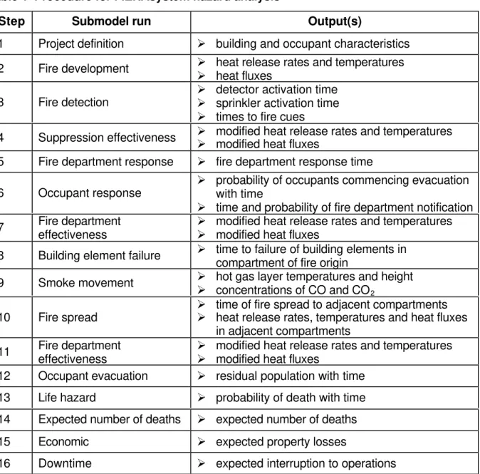
Table 1 Procedure for FIERAsystem hazard analysis

Step Submodel run Output(s)

1 Project definition Ø building and occupant characteristics 2 Fire development Ø heat release rates and temperatures

Ø heat fluxes

3 Fire detection Ø detector activation time_{Ø sprinkler activation time} Ø times to fire cues

4 Suppression effectiveness Ø modified heat release rates and temperatures Ø modified heat fluxes

5 Fire department response Ø fire department response time

6 Occupant response Ø probability of occupants commencing evacuationwith time Ø time and probability of fire department notification 7 Fire department

effectiveness Ø modified heat release rates and temperatures_{Ø modified heat fluxes} 8 Building element failure Ø time to failure of building elements in

compartment of fire origin

9 Smoke movement Ø hot gas layer temperatures and height Ø concentrations of CO and CO2

10 Fire spread Ø time of fire spread to adjacent compartments_{Ø heat release rates, temperatures and heat fluxes} in adjacent compartments

11 Fire department effectiveness

Ø modified heat release rates and temperatures Ø modified heat fluxes

12 Occupant evacuation _{Ø residual population with time} 13 Life hazard Ø probability of death with time 14 Expected number of deaths _{Ø expected number of deaths} 15 Economic Ø expected property losses

(23)

(24)

Select Scenario Fire Department Response Model Calculate fire department response time

Occupant Response Model

Calculate time of fire department notification Calculate probability of fire department notification Calculate probability of occupant response(t)

Fire Department Effectiveness Model

Calculate FD suppressed HRR(t) and plume temp's(t) Calculate FD suppressed heat fluxes(t,c) Start Hazard Analysis End Hazard Analysis Suppression Effectiveness Model

Calculate sprinkler suppressed heat

fluxes(t,r)

Modify time to critical heat flux Calculate sprinkler suppressed HRR(t) and plume temp's(t) Detection Model Calculate sprinkler activation time Calculate time of fire cue Calculate smoke detection time

Fire Development Model

Calculate heat flux(t,r)

Calculate time to critical heat flux Calculate heat release rate(t) and plume temperatures(t) Economic Model Calculate cost of damage to building(c) Calculate cost of damage to contents(c) Expected Number of Deaths Model

Calculate number of occupants who have died(t,c) Calculate residual population(t,c) Calculate number of occupants who have exited(t,c)

Life Hazard Model

Calculate probability of death(t,c) Occupant Evacuation Model Calculate probability of exit(t,c) Building Element Failure Model Calculate time of failure of COF building elements

Fire Spread Model Calculate HRR and plume temp's of fire in adjacent compartments (t,c) Calculate heat flux of adjacent compartments (t,r,c) Smoke Movement Model

Calculate CO2(t,c) and

CO(t,c) concentrations

Calculate time to fire ignition from

hot gasses(c) Interface

height(t,c), lower layer temp.(t,c), and upper layer

temp.(t,c)

(25)

(26)

Start Risk Analysis Get input

Loop through possible fires

Last possible fire?

Calculate Probability of Scenario Occurrence, P(Sc)i Calculate Expected Number of Deaths Calculate Probable Fire Losses Possible fires & probabilities

Probability of fire dept. arrival

Probability of suppression system activation Building life and interest rate

Cost of building and contents Cost of Fire Protections systems

Sum Risk to Life and Risk of Fire

Losses

Calculate Fire Cost Expectation

Hazard Analysis

Write ERL & FCE to output

End Risk Analysis

No

Yes

Loop through Fire Department & Suppression system combinations Last FD & SS combination? No Yes

Fire Department Arrives Fire Department does not Arrive Suppression system activates Suppression system does not activate

(27)

5. CONCLUSIONS

A new computer model, FIERAsystem, has been developed to evaluate risk from fires in light industrial buildings using a systems approach. FIERAsystem has been developed as a tool to assist fire protection engineers, building officials, fire service personnel and

researchers, and can be used to conduct hazard and risk analyses, and to evaluate whether a selected design satisfies established fire safety objectives. While the model is primarily designed for use in warehouses and aircraft hangars, it can be modified for application to other industrial buildings.

The new-developed FIERAsystem provides great capabilities and flexibility in conducting hazard and risk assessments. Individual submodels of FIERAsystem could be used as stand-alone models or collectively to evaluate fire safety in a building.

(28)

6. REFERENCES

1. Yung, D., Hadjisophocleous, G.V., Proulx, G. and Kyle, B.R., "Cost-Effective Fire-Safety Upgrade Options for a Canadian Government Office Building", Proceedings,

International Conference on Performance-Based Codes and Design Methods, 1996, Ottawa, ON, pp. 269–280

2. Hadjisophocleous, G.V., Benichou, N., Torvi, D.A. and Reid, I.M.A., “Evaluating

Compliance of Performance-Based Designs with Fire Safety Objectives”, Proceedings,, 3rd International Conference on Performance-Based Codes and Fire Safety Design Methods, 2000, Lund University, Sweden.

3. Fu, Z. and Hadjisophocleous, G.V., “A Two-Zone Fire Growth and Smoke Movement Model for Multi-Compartment Buildings”, Fire Safety Journal, Vol. 34, 2000, pp. 257-285. 4. Torvi, D.A., Raboud, D.W., and Hadjisophocleous, G.V., “FIERAsystem Theory Report:

Life Hazard Model”, IRC Internal Report No. 781, Institute for Research in Construction, National Research Council of Canada, Ottawa, ON, 1999.

5. SFPE Handbook of Fire Protection Engineering, Second Edition, National Fire Protection Association, Quincy, MA, 1995.

6. Evans, D.D., “Ceiling Jet Flows”, SFPE Handbook of Fire Protection Engineering, Second Edition, National Fire Protection Association, Quincy, MA, 1995 pp. 2-32–2-39. 7. Mudan, K.S. and Croce, P.A., “Fire Hazard Calculations for Large Open Hydrocarbon

Pool Fires”, SFPE Handbook of Fire Protection Engineering, Second Edition, National Fire Protection Association, Quincy, MA, 1995, pp. 3-197–3-240.

8. Alpert, R.L. and Ward, E.J., “Evaluation of Unsprinklered Fire Hazards”, Fire Safety Journal, Vol. 7, 1984, pp. 127-143.

9. Yager, B., Kashef, A., Benichou, B., and Hadjisophocleous, G.V., “FIERAdetection Model (DTRM) Theory Report,” IRC Internal Report No. 841, Institute for Research in Construction, National Research Council Canada, Ottawa, ON, 2002.

10. Proulx, G., "Evacuation Time and Movement in Apartment Buildings", Fire Safety Journal, Vol. 24, 1995, pp. 229–246.

11. Tsao, C.K. and Perry, W.W., “Modifications to the Vulnerability Model: A Simulation System for Assessing Damage Resulting from Marine Spills (VM4)”, Report CG-D-38-79, U.S. Coast Guard Office of Research and Development, Washington, DC,1979. 12. Eisenberg, N.A., et al., “Vulnerability Model: A Simulation System for Assessing

Damage Resulting from Marine Spills (VM1)”, Report CG-D-137-75 (NTIS AD-A015 245), U.S. Coast Guard Office of Research and Development, Washington, DC, 1975. 13. Hadjisophocleous, G.V. and Yung, D., “A Model for Calculating the Probabilities of

Smoke Hazard from Fires in Multi-Storey Buildings”, Journal of Fire Protection Engineering, Vol. 4, 1992, pp. 67-80.

14. Purser, D.A., “Toxicity Assessment of Combustion Products”, SFPE Handbook of Fire Protection Engineering, Second Edition, National Fire Protection Association, Quincy, MA, 1995, pp. 2-85-2-146.

15. Torvi, D.A., Hadjisophocleous, G.V., and Hum, J., “A New Method for Estimating the Effects of Thermal Radiation from Fires on Building Occupants”, accepted for

(29)

presentation at the ASME 2000 International Mechanical Engineering Congress and Exposition, 2000, Orlando, FL.

16. David Torvi, Ahmed Kashef, Noureddine Benichou, and George Hadjisophocleous, “FIERAsystem Water Requirements Model (WTRM)”, Fire Risk Management Program, Institute for Research in Construction, National Research Council Canada, Internal Report 851, May 2002.

17. National Building Code of Canada 1995, Canadian Commission on Building and Fire Codes, National Research Council of Canada, Ottawa, ON, 1995.

(30)

APPENDIX A – CASE STUDY  FIERAsystem ANALYSIS OF A SUPPLY BUILDING

To demonstrate the use of FIERAsystem, a case study analysis of a supply building is being performed. The building will be referred to, in this report, as the “Supply Building”. The study will include an analysis of fire and smoke spread in the building, and the

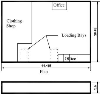
evacuation of occupants. The Supply Building includes two main areas, namely, the older and the new sections on the south and the north sides of the building, respectively. The presence of fire and barrier walls between the original and the addition north sections allows the Supply Building to be modelled using only the older portion of the building. The older section includes a large shipping and receiving area with loading bays. There is also a clothing shop and offices. The offices and clothing shop areas have two levels. Figure A1 shows the floor plan and elevation of the compartments being modelled. In the

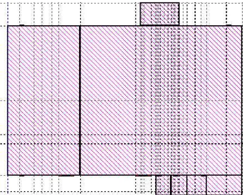
FIERAsystem simulation, the Supply Building has been simplified by using the equivalent volumes of building space, as seen in Figure A2. Placing the offices outside the building, while simplifying the computations, does not affect the accuracy of the model predictions. It should be noted that the travel paths for occupants of the offices were determined in

accordance to the actual locations of the offices. All internal doors are assumed open and all external doors are assumed closed.

One possible location for a fire is the main floor western office. This office consists of standard office materials such as desks, files, and chairs. Another possible location for a fire is the clothing shop. Many military clothing articles are stored and distributed in this location. Clothing Shop Office Office Plan Elevation

All dimensions are in metres.

Loading Bays

(31)

Figure A2 Compartments Modelled using FIERAsystem

Fire Scenarios

A potential fire scenario occurs in the western office. The office has a floor area of 31.44 m2. There are two windows to the exterior and two interior windows and a door. A medium t2 fire is assumed to represent this fire scenario. The fire is assumed to occur in the centre of the room and is estimated to reach a maximum heat release rate of 11 MW at 980 s. The heat release rate curve is shown in Figure A3.

Fire Development

Figure A3 shows the heat release rate curve for the western office, predicted by the fire development submodel. The fire is estimated to reach flashover at 580 s, and the maximum heat release rate of 11 MW at 980 s.

(32)

0 2000 4000 6000 8000 10000 12000 0 200 400 600 800 1000 1200 1400 1600 1800 2000 Time (s)

Heat Release Rate (kW)

Figure A3 Predicted Heat Release Curve for the 11 MW Fire in the Western Office

Detection and Suppression

The fire is assumed to be located in the middle of the office and underneath a combination detector. The detector is assumed to have an RTI of 33 m1/2s1/2, an activation temperature of 57

°

C or activation rate of rise of 8 °C/s. There are no sprinklers in the western office. The detector in the office is predicted to activate at 62 s after ignition. The series of sprinklers located in the main loading area and the clothing shop were not

activated in the analysis.

Fire Department Response and Effectiveness

The fire department is assumed to be notified by an automatic alarm that sounds with the activation of the detector. The fire department is located on the military base, 0.5 km away from the Supply Building. The fire department response submodel calculates the dispatch, preparation, and travel time to be 110 s, 231 s, and 78 s, respectively. When these times are added to the notification time of 62 s, determined by the time of detector activation, it is predicted that the fire department will respond in 481 s. The fire department is expected to set up within 300 s. Therefore, the fire department intervention time is 781s.

The effectiveness of the fire department is expected to affect the results of the simulation as the predicted intervention time (781 s) occurs prior to reaching the peak heat release rate (980s).

Occupant Response

It is assumed that there are 17 occupants in the building. As shown in Figure A4, all occupants in the compartment of fire origin are predicted to take action in approximately 300 s, and all occupants in the remaining compartments are predicted to take action in

approximately 700 s. The time the fire department would be notified by an occupant is compared with the time that the fire department is notified due to the activation of the

(33)

that the fire department is automatically notified when the detector activates at 62 s.

Therefore, the notification time calculated by the occupant response submodel is not used in the current calculations.

0 0.1 0.2 0.3 0.4 0.5 0.6 0.7 0.8 0.9 1 0 200 400 600 800 1000 1200 1400 1600 1800 2000 Time (s)

Probability of Occupant Action

Compartment of Fire Origin Adjacent Compartment Other Compartment