TEX twocolumn style in AASTeX63
The LSST DESC DC2 Simulated Sky Survey
THELSST DARKENERGYSCIENCECOLLABORATION(LSST DESC)
BELAABOLFATHI,1DAVIDALONSO,2ROBERTARMSTRONG,3ÉRICAUBOURG,4HUMNAAWAN,5, 6YADUN. BABUJI,7, 8
FRANZERIKBAUER,9, 10, 11RACHELBEAN,12GEORGEBECKETT,13RAHULBISWAS,14JOANNER. BOGART,15, 16
DOMINIQUEBOUTIGNY,17KYLECHARD,7, 8JAMESCHIANG,15, 16CHUCKF. CLAVER,18JOHANNCOHEN-TANUGI,19, 20
CÉLINECOMBET,21A
NDREWJ. CONNOLLY,22 S
COTTF. DANIEL,22S
ETHW. DIGEL,15, 16A
LEXDRLICA-WAGNER,23, 24, 25 RICHARDDUBOIS,15, 16E MMANUELGANGLER,20E RICGAWISER,5T HOMASGLANZMAN,15, 16 P HILLIPEGRIS,20S ALMANHABIB,7 ANDREWP. HEARIN,7K ATRINHEITMANN,7F ABIOHERNANDEZ,26R ENÉEHLOŽEK,27, 28J OSEPHHOLLOWED,7M USTAPHAISHAK,29 ŽELJKOIVEZI ´C,30MIKEJARVIS,31SAURABHW. JHA,5STEVENM. KAHN,15, 16, 18, 32J. BRYCEKALMBACH,22
HEATHERM. KELLY,15, 16EVEKOVACS,7 DANILAKORYTOV,7, 8K. SIMONKRUGHOFF,18CRAIGS. LAGE,33FRANÇOISLANUSSE,34
PATRICIALARSEN,7L
AURENTLEGUILLOU,35N
ANLI,36E
MILYPHILLIPSLONGLEY,37R
OBERTH. LUPTON,38
RACHELMANDELBAUM,39Y
AO-YUANMAO,5 ,*PHILMARSHALL,15, 16J
OSHUAE. MEYERS,3M
ARCMONIEZ,40 CHRISTOPHERB. MORRISON,30A
NDREINOMEROTSKI,41P
AULO’CONNOR,41H
YEYUNPARK,41J IWONPARK,15, 32, 16 JULIENPELOTON,40 D ANIELPERREFORT,42, 43J AMESPERRY,13S TÉPHANEPLASZCZYNSKI,40A DRIANPOPE,7 ANDREWRASMUSSEN,15, 16K EVINREIL,15, 16A ARONJ. ROODMAN,15, 16E LIS. RYKOFF,15, 16 F. J AVIERSÁNCHEZ,1, 23 SAMUELJ. SCHMIDT,33D ANIELSCOLNIC,44C HRISTOPHERW. STUBBS,45 J. A NTHONYTYSON,33T HOMASD. URAM,7 ANTONIOVILLARREAL,7C HRISTOPHERW. WALTER,44M ATTHEWP. WIESNER,46W. M
ICHAELWOOD-VASEY,42, 43J
OEZUNTZ,47 1Department of Physics and Astronomy, University of California, Irvine, Irvine, CA 92697, USA
2Department of Physics, University of Oxford, Denys Wilkinson Building, Keble Road, Oxford OX1 3RH, United Kingdom 3Lawrence Livermore National Laboratory, Livermore, CA 94550, USA
4Université de Paris, CNRS, CEA, Astroparticule et Cosmologie, F-75013 Paris, France
5Department of Physics and Astronomy, Rutgers, The State University of New Jersey, Piscataway, NJ 08854, USA 6Leinweber Center for Theoretical Physics, Department of Physics, University of Michigan, Ann Arbor, MI 48109, USA
7Argonne National Laboratory, Lemont, IL 60439, USA 8University of Chicago, Chicago, IL 60637, USA
9Instituto de Astrofísica and Centro de Astroingeniería, Facultad de Física, Pontificia Universidad Católica de Chile, Casilla 306, Santiago 22, Chile 10Millennium Institute of Astrophysics (MAS), Nuncio Monseñor Sótero Sanz 100, Providencia, Santiago, Chile
11Space Science Institute, 4750 Walnut Street, Suite 205, Boulder, Colorado 80301 12Department of Astronomy, Cornell University, Ithaca, NY 14850, USA
13EPCC, University of Edinburgh, United Kingdom
14The Oskar Klein Centre for Cosmoparticle Physics, Stockholm University, AlbaNova, Stockholm, SE-106 91, Sweden 15SLAC National Accelerator Laboratory, Menlo Park, CA 94025, USA
16Kavli Institute for Particle Astrophysics and Cosmology, Stanford University, Stanford, CA 94305, USA 17Univ. Grenoble Alpes, Univ. Savoie Mont Blanc, CNRS, LAPP, 74000 Annecy, France
18Rubin Observatory Project Office, 950 N. Cherry Ave., Tucson, AZ 85719, USA 19Univ. Montpellier, CNRS, LUPM, 34095 Montpellier, France
20LPC, IN2P3/CNRS, Université Clermont Auvergne, F-63000 Clermont-Ferrand, France 21Univ. Grenoble Alpes, CNRS, LPSC-IN2P3, 38000 Grenoble, France
22DIRAC Institute and Department of Astronomy, University of Washington, Seattle, WA 98195, USA 23Fermi National Accelerator Laboratory, PO Box 500, Batavia, IL 60510, USA
24University of Chicago, Chicago IL 60637, USA
25Kavli Institute for Cosmological Physics, University of Chicago, Chicago, IL 60637, USA 26CNRS, CC-IN2P3, 21 avenue Pierre de Coubertin CS70202, 69627 Villeurbanne cedex, France 27David A. Dunlap Department of Astronomy and Astrophysics, 50 St. George Street, Toronto ON M5S3H4
28Dunlap Institute for Astronomy and Astrophysics, 50 St. George Street, Toronto ON M5S3H4 29Department of Physics, The University of Texas at Dallas, Richardson, TX 75080, USA 30Department of Astronomy, University of Washington, Box 351580, Seattle, WA 98195, USA
31Department of Physics & Astronomy, University of Pennsylvania, 209 South 33rd Street Philadelphia, PA 19104-6396, USA 32Department of Physics, Stanford University, Stanford, CA 94305, USA
33University of California-Davis, Davis, CA 95616, USA
34AIM, CEA, CNRS, Université Paris-Saclay, Université Paris Diderot, Sorbonne Paris Cité, F-91191 Gif-sur-Yvette, France 35Sorbonne Université, CNRS, IN2P3, Laboratoire de Physique Nucléaire et de Hautes Énergies, LPNHE, 75005 Paris, France
36School of Physics and Astronomy, University of Nottingham, University Park, Nottingham, NG7 2RD, United Kingdom 37Department of Physics, Duke University, Durham NC 27708, USA
38Princeton University, Princeton, NJ, USA
39McWilliams Center for Cosmology, Department of Physics, Carnegie Mellon University, Pittsburgh, PA 15213, USA 40Université Paris-Saclay, CNRS/IN2P3, IJCLab, Orsay, France
41Brookhaven National Laboratory, Upton, NY 11973, USA
42Department of Physics and Astronomy, University of Pittsburgh, Pittsburgh, PA 15260, USA
43Pittsburgh Particle Physics, Astrophysics and Cosmology Center (PITT PACC), University of Pittsburgh, Pittsburgh, PA 15260, USA 44Department of Physics, Duke University, Durham NC 27708, USA
45Dept. of Physics and Dept. of Astronomy, Harvard University, Cambridge, MA 02138, USA 46Benedictine University, Lisle, IL, 60532, USA
47Institute for Astronomy, University of Edinburgh, Edinburgh EH9 3HJ, United Kingdom
Abstract
We describe the simulated sky survey underlying the second data challenge (DC2) carried out in preparation for analysis of the Vera C. Rubin Observatory Legacy Survey of Space and Time (LSST) by the LSST Dark Energy Science Collaboration (LSST DESC). Significant connections across multiple science domains will be a hallmark of LSST; the DC2 program represents a unique modeling effort that stresses this interconnectivity in a way that has not been attempted before. This effort encompasses a full end-to-end approach: starting from a large N-body simulation, through setting up LSST-like observations including realistic cadences, through image simulations, and finally processing with Rubin’s LSST Science Pipelines. This last step ensures that we generate data products resembling those to be delivered by the Rubin Observatory as closely as is currently possible. The simulated DC2 sky survey covers six optical bands in a wide-fast-deep (WFD) area of approximately 300 deg2 as well as a deep drilling field (DDF) of approximately 1 deg2. We simulate 5 years of the planned 10-year
survey. The DC2 sky survey has multiple purposes. First, the LSST DESC working groups can use the dataset to develop a range of DESC analysis pipelines to prepare for the advent of actual data. Second, it serves as a realistic testbed for the image processing software under development for LSST by the Rubin Observatory. In particular, simulated data provide a controlled way to investigate certain image-level systematic effects. Finally, the DC2 sky survey enables the exploration of new scientific ideas in both static and time-domain cosmology. Keywords:methods: numerical – large-scale structure of the universe
1. INTRODUCTION
In the coming decade, several large sky surveys will collect new datasets with the aim of advancing our understanding of fundamental cosmological physics well beyond what is cur-rently possible. In the language of the Dark Energy Task Force (DETF, Albrecht et al. 2006), Stage IV dark energy surveys such as the Dark Energy Spectroscopic Instrument (DESI) survey1 (DESI Collaboration et al. 2016), the Vera
C. Rubin Observatory Legacy Survey of Space and Time (LSST)2 (LSST Science Collaboration et al. 2009; Ivezi´c
et al. 2019), the Euclid survey3(Laureijs et al. 2011), and the
Nancy Grace Roman Space Telescope survey4(Spergel et al.
2015;Dore et al. 2019) promise to transform our
understand-ing of basic questions such as the cause of the accelerated
ex-*NASA Einstein Fellow
1 www.desi.lbl.gov/the-desi-survey 2 www.lsst.org
3 www.cosmos.esa.int/web/euclid,www.euclid-ec.org 4 roman.gsfc.nasa.gov
pansion rate of the Universe. The LSST Dark Energy Science Collaboration (DESC5) was formed in 2012 (LSST Dark
En-ergy Science Collaboration 2012) to prepare for studies of
fundamental cosmological physics with the Vera C. Rubin Observatory LSST. DESC plans an ambitious scientific pro-gram including joint analysis of five dark energy probes that are complementary in constraining power within the cosmo-logical parameter space and in handling systematic uncer-tainties, and together result in Stage IV-level constraints on dark energy (The LSST Dark Energy Science Collaboration
et al. 2018). The challenge faced by the LSST DESC is to
build software pipelines to analyze the released LSST data products and unlock the statistical power of the LSST dataset while robustly constraining systematic uncertainties. More-over, these pipelines must work at scale on a dataset that is substantially beyond current surveys in size and complexity.
To meet this challenge, the DESC is iteratively developing analysis pipelines based on the current state of the art and
then analyzing simulations and precursor data in a series of “data challenges” (DCs) that increase in scope and complex-ity. The first data challenge (DC1) is described inSánchez
et al.(2020); in DC1 a full end-to-end simulation pipeline to
generate LSST-like data products was implemented. DC1 covered ten years of data taking in an area of ≈40 deg2
and the simulations were carried out in r-band only. The input catalog for DC1 was based on the Millennium sim-ulation semi-analytic galaxy catalog (Springel et al. 2005), which is embedded in the LSST catalog simulation frame-work, CatSim (Connolly et al. 2010,2014). Image simula-tions were carried out with imSim (DESC, in preparation), and the resulting dataset was then processed with the Ru-bin’s LSST Data Management Science Pipelines software stack6(throughout the paper we refer to it as LSST Science Pipelines), developed by the Rubin’s LSST Data Manage-ment (DM) team. The main focus in DC1 was the investi-gation of systematic effects relevant for large-scale structure measurements (the galaxy catalog within CatSim does not provide shear measurements), as well as the validation and verification of its end-to-end workflow.
In this paper, we describe the second data challenge (DC2) which goes well beyond DC1 in several ways. Working groups within DESC plan to use DC2 for tests of many pro-totype analysis pipelines that are being developed. A selec-tion of these includes pipelines for measuring weak gravi-tational lensing correlations, large-scale structure statistics, galaxy cluster abundance and masses based on weak lensing, supernova light curve recovery, and inference of ensemble redshift distributions for samples based on photometric red-shifts. To optimize the scientific return of LSST, individual probes cannot be treated in isolation; cross-correlations be-tween them must be properly understood and exploited to sharpen obtainable results as well as to open new avenues of discovery. In order to enable tests across a broad range of sci-ence cases, DC2 covers all six optical bands ugrizy that will be observed by the LSST and the area compared to DC1 is in-creased by a factor of 7.5 to ≈300 deg2to strike a balance
be-tween computational cost and analysis value. Another major development compared to DC1 is the integration of a new ex-tragalactic catalog, called cosmoDC2, described inKorytov
et al.(2019). Based on the Outer Rim simulation (Heitmann
et al. 2019), which has 200 times the volume of the
Millen-nium run (Springel et al. 2005), cosmoDC2 not only covers a large area to encompass the 300 deg2required for DC2 but
also includes shear measurements and employs an enhanced galaxy modeling approach. A new interface to CatSim was developed, followed by a workflow for the image simulation generation analogous to DC1. The technical implementation of the workflow itself was completely redone to enable scal-ing to thousands of compute nodes.
Carrying out an ambitious program such as the one de-scribed here requires many careful tests, code optimization and validation, and efficient workflow designs. In order to
6 pipelines.lsst.io
accomplish this complex set of tasks, we implemented a staged series of activities, following the strategy that would be used for an actual survey: We first executed the equiva-lent of an engineering run to then advance to a science-grade run. The engineering run, or Run 1, had several stages in which we developed and implemented the full end-to-end pipeline, tested our new approach for generating an extra-galactic catalog, investigated two different image simulation tools, PhoSim (Peterson et al. 2015) and imSim, processed the simulated images using the LSST Science Pipelines, and created a set of tutorials for the collaboration to enable mem-bers to start interacting with the data products. The engineer-ing runs covered a limited area of 25 deg2out to redshift z = 1
and were used to identify and eliminate many shortcomings in the overall set-up. Run 2, one of two science-grade runs, covers the full target area of DC2: a 300 deg2 patch out to
z= 3. The other science-grade run, Run 3, covers the Deep Drilling Field (DDF), a 1 deg2patch within the 300 deg2that
contains additional time-varying objects. In this paper we focus on Runs 2 and 3 but provide information about Run 1 wherever useful.
The paper is organized as follows. First, inSection 2, we describe the requirements on the extragalactic components for DC2 as set by the needs of the relevant probes of cosmic acceleration. Next, inSection 3we describe details regard-ing the DC2 survey design and the observregard-ing cadence. The DC2 survey includes a wide-fast-deep (WFD) area as well as a DDF.Section 4provides an overview of the end-to-end workflow we have implemented. Detailed descriptions of the different workflow steps are provided in the following sec-tions: starting with the generation of the extragalactic catalog and the input catalogs for the image simulations (Section 5), to the image simulations themselves inSection 6, to the final image processing inSection 7. The resulting data products and our data access strategy are detailed in Section 8 and
Section 9. We conclude inSection 10. Finally,Appendix A
provides an overview of the calibration products required to for the data processing with the LSST Science Pipelines, and
Appendix Bsummarizes the acronyms and the main
simula-tion packages used in the paper.
2. DC2 REQUIREMENTS
The generation of an end-to-end survey simulation, from extragalactic catalogs to processed data products that can be used to test analysis methodology, is a very ambitious under-taking. When designing and planning such a project, several competing considerations must be taken into account. For each component in the simulation we evaluate whether real-istic models based on first principles are available and feasi-ble to implement within our availafeasi-ble human and computing resources, or whether we must use approximate or empiri-cal models. LSST will enter new observational territory and we have to decide what approximations (if any) we need to predict the unexplored data – for example, the galaxy pop-ulations that will be observed by LSST clearly cannot be predicted from first principles, but rather require approxi-mate modeling approaches and some degree of extrapolation
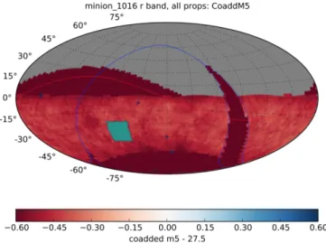
Figure 1. Image of the sky along with possible coverage by LSST observations (red, Jones et al. 2015) from the minion_1016 sur-vey simulation shown in Aitoff projection. The blue line marks the Galactic equator and the red line the Ecliptic. More details are pro-vided in Section 3. The green region shows the area on the sky that is covered by DC2 and is simply overlaid on the coadded depth skymap.
from current observations. When undertaking detailed im-age simulations, we may accept approximate models to real-ize substantial computational efficiencies while still enabling the majority of our expected use cases. Finally, the LSST Science Pipelines are still under very active development. Therefore, we may exclude certain effects from the simula-tions if the current version of the LSST Science Pipelines cannot account for them and if they would dominate over smaller effects that are of interest to us.
When DC2 was conceived, the LSST DESC working groups put forward a range of requirements to enable many tests and science investigations that they planned to carry out with DC2. When deciding which features would be truly im-portant for DC2, the interplay between cost and benefit had to be carefully considered, given available time and resources.
In the following we provide an overview of the basic re-quirements for DC2 in Section 2.1, including size, depth and simulated survey duration, followed by a discussion of the science requirements as put forward by the LSST DESC working groups inSection 2.2. We will carefully highlight which science requirements have been met and which remain to be met in future simulation campaigns.
2.1. Basic Requirements
The DC2 Universe aims to capture a small, representative area of the sky as observed in the LSST.Figure 1shows the area that DC2 covers in comparison to an earlier baseline LSST footprint. Basic specifications for the generation of DC2 concern the size of the simulated area, the number of survey years to be simulated, the bands to be included, and the redshift range to be covered.
The DC2 area spans 300 deg2. This size provides a good
compromise between computational cost for the image simu-lations and processing and areal size sufficient to derive cos-mological constraints for weak lensing and large-scale struc-ture measurements. The area is similar to areas covered by Stage II and early Stage III surveys and therefore has been proven to enable meaningful cosmological investigations.
When considering the number of years in the survey to simulate, the cost of the image simulations and also the cost for the processing of the data were taken into account. The working groups requested several survey years to investigate improvements of cosmological constraints over time. The difference between 5 and 10 survey years was viewed as hav-ing a minor effect on this study; the difference between one and five years of observations, however, in terms of not only depth but also the homogeneity of the dataset, is consider-able.
The number of bands simulated strongly affects the com-putational requirements for the image simulations. It was decided that the opportunities for science projects with DC2 were greatly enhanced if all bands were included.
Finally, the redshift reach and magnitude limits needed to be set. Here, the biggest challenge is the modeling capability for the extragalactic catalog that underlies DC2. Very faint galaxies, for example, require an extremely high resolution simulation. Our approach for cosmoDC2 is based partly on an empirical modeling strategy and approximations had to be implemented for high-redshift galaxies. An extensive dis-cussion of these challenges and how they were overcome is given inKorytov et al.(2019).
2.2. Science Considerations
The DC2 Universe has several different components that are important for LSST DESC to enable the science and pipeline tests that will prepare the collaboration for data arrival. First, a representative extragalactic component is needed that covers many features of the actual observed galaxy distribution, including realistic colors, sizes and shapes, and accurate spatial correlations. In addition, the DC2 Universe also includes our local neighborhood, e.g., Milky Way stars and galactic reddening. For this we employ a range of observational data provided via the LSST soft-ware framework CatSim (Connolly et al. 2010,2014). Since LSST is a ground-based survey, observing conditions from the ground also need to be modeled for each 30 second in-tegration, which is referred to as a “visit”. Finally, the tele-scope and the camera add a number of instrumental effects to the images that have to be either corrected or compensated for. In DC2, the aim is to capture all of these components – the extragalactic and local environments, observing condi-tions from the ground and instrumental and detector artifacts. We defer the detailed discussion of our implementation of ef-fects due to the local environment and observations to
Sec-tion 5.
In this section we focus on the science considerations for the DC2 Universe to investigate probes of cosmic accelera-tion relevant to LSST DESC. For a comprehensive review of
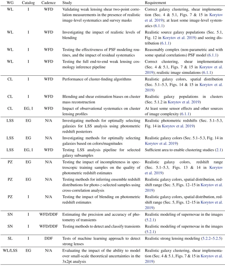
Table 1. DC2 science opportunities, and simulation requirements to enable those opportunities, for different LSST DESC Working Groups. ‘I’ denotes the image catalog and ‘EG’ the extragalactic catalog. The working group acronyms are: WL – weak lensing, CL – clusters, LSS – large-scale structure, PZ – photo-z, SN – supernova, SL – strong lensing. The entry for ‘cadence’ indicates either WFD or DDF for the science cases using image simulations, or N/A for those science cases that primarily rely on the extragalactic catalog. The ‘Requirement’ column also includes a link to the section in this paper or reference to other papers where readers can learn about the feature implementation intended to produce simulations that meet this requirement.
WG Catalog Cadence Study Requirement
WL I WFD Validating weak lensing shear two-point corre-lation measurements in the presence of realistic image-level systematics and survey masks
Correct galaxy clustering, shear implementa-tion (Sec. 4 & 5.1, Figs. 7 & 15 in Korytov et al. 2019); at least some image-level system-atics (6.1.1)
WL I WFD Investigating the impact of realistic levels of blending
Realistic source galaxy populations (Sec. 5.1, Fig. 12 inKorytov et al. 2019) and seeing dis-tribution (6.1.1)
WL I WFD Testing the effectiveness of PSF modeling rou-tines, and the impact of residual systematics
Reasonably complex (non-parametric and with some spatial correlations) PSF model (6.1.1) WL I WFD Testing the full end-to-end weak lensing
cos-mology inference pipeline
Correct clustering, shear implementation (Sec. 4 & 5.1, Figs. 7 & 15 inKorytov et al. 2019); realistic image simulations (6.1.1) CL I WFD Performance of cluster-finding algorithms Realistic galaxy colors, spatial distribution
(Sec. 5.1–5.3, Figs. 14 & 15 inKorytov et al. 2019)
CL I WFD Blending and shear estimation biases on cluster mass reconstruction
Realistic galaxy populations in clusters (Sec. 5.1.2 inKorytov et al. 2019)
CL EG, I WFD Impact of observational systematics on cluster lensing profiles
At least some sensor effects and other sources of image complexity (6.1.1)
LSS EG N/A Investigating methods for optimally selecting galaxies for LSS analysis using photometric redshift posteriors
Realistic photometric redshifts (Sec. 5.1–5.3, Fig. 14 inKorytov et al. 2019)
LSS EG N/A Investigating methods for optimally selecting galaxies based on colors/magnitudes
Realistic galaxy colors (Sec. 5.1–5.3, Fig. 14 in
Korytov et al. 2019) LSS EG, I WFD Testing LSS analysis pipeline for selected
galaxy subsamples
Sufficient area to enable clustering studies (2.1)
PZ EG N/A Testing the impact of incompleteness in spec-troscopic training samples on the quality of photometric redshift estimates
Realistic galaxy colors, redshift range (Sec. 5.1–5.3, Figs. 13 & 14 in Korytov et al. 2019)
PZ EG N/A Testing methods for inferring ensemble redshift distributions for photo-z-selected samples using cross-correlation analysis
Realistic galaxy colors, spatial distribution, red-shift range (Sec. 5, Figs. 12–15 inKorytov et al. 2019)
PZ I N/A Testing the impact of blending on photometric redshift estimates
Realistic galaxy colors, spatial distribution, red-shift range (Sec. 5, Figs. 12–15 inKorytov et al. 2019)
SN I WFD/DDF Estimating the precision and accuracy of pho-tometry of transients
Realistic modeling of supernovae in the images (5.2.1)
SN I WFD/DDF Testing methods to detect and classify transients Realistic modeling of supernovae in the images (5.2.1)
SL I DDF Tests of machine learning approach to detect strong lenses
Realistic strong lensing modeling (5.2.2–5.2.5)
WL/LSS EG N/A Evaluating the impact of the ability to model over small-scale theoretical uncertainties in the 3x2pt analysis
Realistic galaxy clustering, shear implementa-tion (Sec. 4 & 5.1, Figs. 7 & 15 inKorytov et al. 2019)
observational probes of cosmic acceleration, see, e.g.,
Wein-berg et al.(2013). For an LSST DESC specific discussion,
we refer the reader to the LSST DESC Science Requirements Document (The LSST Dark Energy Science Collaboration
et al. 2018). The LSST DESC working groups that focus on
cosmological probes and photometric redshifts provided a set of considerations that drove the design of the simulated sur-vey as summarized inTable 1. These are further discussed in this section.
2.3. Weak Lensing
Weak gravitational lensing is sensitive to the geometry of the Universe and to the growth of structure as a function of time (for a recent review, seeKilbinger 2015). Cosmological weak lensing analysis involves measuring the minute distor-tions of faint background galaxies that are induced by the gravitational potential of the matter distribution located be-tween the source galaxies and the observer. Weak lensing is hence sensitive to both dark and luminous matter alike, as it does not rely on luminous tracers of the dark matter density field. However, achieving robust cosmological con-straints from weak lensing requires exquisite control of ob-servational and astrophysical systematic effects. Simulations that are tailored to the survey at hand are one important ingre-dient in systematics mitigation. For a recent, comprehensive overview of all sources of systematic uncertainty in cosmo-logical weak lensing measurements, see, e.g.,Mandelbaum
(2018). The papers presenting the weak lensing catalogs and cosmological weak lensing analyses from ongoing surveys provide examples of how the key systematics are character-ized and mitigated in practice (e.g.,Zuntz et al. 2018;Abbott
et al. 2018;Mandelbaum et al. 2018;Hikage et al. 2019;
As-gari et al. 2020;Giblin et al. 2020).
Studying observational systematics such as shear calibra-tion bias and photometric redshift calibracalibra-tion bias requires synthetic catalogs with realistic galaxy shapes, sizes, mor-phologies and colors. It is important that these quantities scale correctly with redshift, and that galaxy color-dependent clustering is included. Blending of the light from spatially overlapping sources is one of the most difficult effects to cor-rect for when measuring the shapes and colors of galaxies (e.g.,Samuroff et al. 2018). Hence it is very important that the clustering has flux, size and color distributions that are well matched to real galaxies to ensure that the full challenge of color-dependent blending due to both chance projections and galaxy clustering is present in the simulations. Color gra-dients in the galaxy spectral energy distribution (SED) and color-dependent galaxy shapes are important to include in order to correctly model the interdependence of measuring shapes in the different photometric bands and to extract the photometric information for a given set of cuts in the catalog
(Kamath et al. 2020).
The point-spread function (PSF) is another critical sys-tematic effect for weak lensing shear calibration (
Paulin-Henriksson et al. 2008). The PSF model must include a
plausible atmospheric turbulent layer to correctly simulate small-scale spatial variations. The atmospheric component
of the PSF in DC2 uses a frozen flow approximation for six atmospheric turbulent layers with plausible heights and outer scales. Optical aberrations lead to complex PSF morphol-ogy and vary across the field of view (FOV), so this also must be simulated accurately. For DC2, we used estimates of the variation in aberrations expected for the residuals from the active optics corrections of the Rubin Observatory LSST Camera (hereafter LSSTCam). Differential chromatic refrac-tion leads to addirefrac-tional chromatic dependence of the PSF and thus is also included (Meyers & Burchat 2015). The brighter-fatter effect (seeDowning et al. 2006for an early discussion of the effect) was also identified as a critical confounding factor for PSF determination and weak lensing shear estima-tion and is therefore included in the DC2 simulaestima-tions (see, e.g.,Gruen et al. 2015for measurements and modeling ap-proaches of this effect for the Dark Energy Camera and
Coul-ton et al. 2018for the Hyper Suprime-Cam). Finally,
accu-rate simulation of the PSF modeling step requires a realistic stellar catalog in terms of stellar density and SEDs, which is part of DC2.
2.4. Clusters
Galaxy clusters, the largest gravitationally bound systems in the Universe, allow us to critically test predictions of struc-ture growth from cosmological models (see, e.g.Allen et al. 2011for an extensive review). Indeed, as identified in the U.S. Department of Energy Cosmic Visions Program (
Do-delson et al. 2016) and other works, “The number of massive
galaxy clusters could emerge as the most powerful cosmo-logical probe if the masses of the clusters can be accurately measured."LSST will provide the premier optical dataset for cluster cosmology in the next decade; over 100,000 clusters extending to redshift z ∼ 1.2 are expected to be detected. The DC2 simulations are designed to enable tests of galaxy clus-ter identification and cosmological analysis.
For galaxy clusters, the most critical requirement is that the simulations accurately capture the photometric properties of the cluster galaxy population (e.g., the dominant red se-quence, evolving blue fraction, luminosity function and spa-tial distribution of cluster members). It is also desirable to capture the photometric properties of galaxies as a function of redshift to enable the study of the effects of line-of-sight projections in galaxy clusters. While a large sky area beyond the 300 deg2 presented here will be required for robust sta-tistical characterization of cluster finding and cosmological pipelines, the DC2 image simulations will enable stringent tests of deblending algorithms in dense environments, which will help improve both photometric redshift and shear esti-mation.
2.5. Large-Scale Structure
The Large-Scale Structure (LSS) working group aims to constrain cosmological parameters from the properties of the observed galaxy clustering. The main source of systematic uncertainty for LSS lies in the details of the connection be-tween the galaxy number density and the underlying dark matter density field. Furthermore, unlike weak lensing, LSS
is a local tracer of the matter distribution, not connected to an integral along a line of sight. The constraining power of LSS is therefore also more sensitive to the quality of photo-metric redshift estimation (see, e.g.,Chaves-Montero et al.
2018;Wright et al. 2020).
For this reason, three important astrophysical factors guide the requirements for LSS. The color distribution of the galaxy sample must be realistic, with relevant subsamples (e.g., red sequence, blue cloud) having number densities in agreement with existing measurements of their luminosity functions, and the clustering properties of these subsamples should also match measured values (e.g.,Wang et al. 2013;Bernardi et al. 2016). These clustering properties should minimally encom-pass the large-scale two-point correlation function, but would ideally include the small-scale clustering and higher-order correlations. Although an accurate modeling of the effects of galaxy assembly bias would also be desirable, it is not a priority at this stage.
The DC2 images also need to reproduce some of the most relevant observational systematics for galaxy cluster-ing. These come in the form of artificial modulations in the observed galaxy number density caused by depth vari-ations and observing conditions (e.g., sky brightness, seeing, clouds; seeAwan et al. 2016). Another important systematic is the spurious contamination from stars classified as galaxies and vice versa. Therefore, the realism of the observed galaxy size, shape and photometry at the image level is also impor-tant. Finally, the effect of Galactic dust absorption on galaxy brightness and colors (e.g.,Li et al. 2017) has to be modeled accurately so that its impact on clustering contamination can be accounted for.
2.6. Supernovae
The main aim of the Supernova (SN) working group is the inference of cosmological parameters using supernovae (SNe) observed during LSST, in conjunction with other LSST cosmological probes as well as external datasets. Cos-mological inference using SNe (Riess et al. 1998;Perlmutter
et al. 1999) proceeds using the distance-redshift relationship
of cosmological models, and exploits the standardizable can-dle property (Phillips 1993;Tripp & Branch 1999) of Type Ia SNe. LSST is expected to significantly increase the sample of Type Ia SNe (The LSST Dark Energy Science Collaboration
et al. 2018) compared to current surveys (e.g.,Betoule et al.
2014;Rest et al. 2014;Scolnic et al. 2018;Jones et al. 2018,
2019;Brout et al. 2019b) which are already systematics
lim-ited. Therefore, an image simulation that provides a truth catalog of the measurable quantities is an excellent resource for studying potential inaccuracies in quantities measured by the LSST Science Pipelines.
The performance of the pipeline in detecting new sources can be characterized by the efficiency and purity of source detections over a range of significance levels, source bright-nesses and reference image depths (Kessler et al. 2015). Since the performance is usually a function of observing con-ditions and environmental properties (e.g., the contrast be-tween the transient brightness and the local surface
bright-ness of the galaxy), it must also be studied in diverse condi-tions. Recent time domain surveys have improved their de-tection performance by using an additional machine learning classifier (Bloom et al. 2012;Goldstein et al. 2015;
Maha-bal et al. 2019) that classifies difference image detections as
real or bogus. The DC2 data can help in the development and investigation of such algorithms. Forced photometry per-formed on the difference images in the science pipelines is used to measure the fluxes in light curves. DC2 also enables the study of bias in such measured fluxes as a function of observational parameters, or truths. In order to use DC2 for such studies, the DC2 cadence (and the distribution of ob-servational properties) and the locations of the SNe (relative to surface brightness) must be representative of realistic data. DC2 is also useful in the development and investigation of al-ternative algorithms for building light curves, such as Scene Modeling Photometry (Astier et al. 2006; Holtzman et al.
2008;Brout et al. 2019a). It additionally allows
investiga-tions of optimal stacking procedures for detecting dimmer, higher redshift SNe from multiple daily visits, which will be particularly relevant in the LSST DDFs. Finally, in or-der to test host association algorithms (Sullivan et al. 2006;
Gupta et al. 2016), it is essential to have a realistic
associ-ation of hosts and offsets from the host locassoci-ation (Gagliano
et al. 2020).
2.7. Strong Lensing
When a variable background source, such as an active galactic nucleus (AGN) or SN, is strongly lensed by a mas-sive object in the foreground, multiple images are observed and the relative time delays between the images can be mea-sured. Strong-lensing time delays provide direct measure-ments of absolute distance, independently of early-universe probes such as the cosmic microwave background (CMB) and local probes using the cosmic distance ladder: they pri-marily constrain the Hubble constant (H0) and, more weakly,
other cosmological parameters (see e.g. Treu & Marshall 2016, for a recent review).
The LSST dataset is projected to contain ∼8,000 de-tectable lensed AGN and ∼130 lensed SNe (Oguri &
Mar-shall 2010). Isolating a pure and complete sample of strong
lenses from billions of other observed objects is a major algo-rithmic and computational challenge for time delay cosmog-raphy. Developing and testing lens detection algorithms op-erating on either the catalog or the pixel level leads to a num-ber of time-domain requirements on the DC2 design. The goal is to enable initial investigations of a catalog-level lens finder that will perform a coarse search for lensed AGN or SNe, before the search can be fine-tuned on the pixel level with more computational resources. This algorithm will be trained on all of the DC2 Object, Source and DIASource ta-bles7, in order to fully explore the time domain information
7 An extensive description of the LSST data products and tables is given in
the Data Products Definition Document, available at this URL:lse-163.lsst. io
provided by LSST. For the DC2-trained algorithm to gen-eralize well to the real LSST data, to first order, the light curves of DC2 lensed AGN and SNe must encode the cor-related lensing time delays across the multiple images. In addition, the deflector galaxy properties, such as size, shape, mass, and brightness, should agree with the observed popula-tion distribupopula-tions. Lastly, the AGN variability model must be realistic, with the variability parameters following empirical correlations with the physical properties of the AGN, such as black hole mass. We note that the DC2 lensed AGN and SNe only include the intrinsic variability, not the additional vari-ability caused by microlensing by the stars in the lens galaxy. It may be possible to add this effect into the light curves in post-processing. Alternatively, we can model the error on the light curves excluding the effect of microlensing by training a light curve emulator on the DC2 data. Given noiseless light curves with microlensing built in, e.g. according to a sepa-rate empirical model, the emulator can then output DC2-like light curves with microlensing included.
The accuracy of time delay measurements directly prop-agates into the accuracy on H0 inference. The ugrizy light
curves in the DC2 DIASource table, with the DM-processed observation noise, should be an improvement on the ones fea-tured in the Time Delay Challenge (Liao et al. 2015), which only had one filter, assumed perfect deblending, and used a simple, uncorrelated, Gaussian noise model. Without object characterization and deblending algorithms that have been tuned for lensed AGN and SNe, we might expect the auto-matically generated DIASource light curves to be blended and sub-optimally measured; if this is the case, the DC2 im-age data will provide a useful testbed for exploring alterna-tive configurations of the LSST Science Pipelines that can support strong lens light curve extraction. As in the lens finding application, time delay estimation requires a realis-tic AGN variability model. For H0 recovery tests, the image
positions and magnification must be consistent with the time delays.
Massive structures close to the lens line of sight cause weak lensing effects that perturb the time delays. Correct-ing for these perturbations is an important part of the cos-mographic analysis and a potential source of significant sys-tematic error. By embedding lensed AGN and SNe in plausi-ble environments, the DC2 dataset will enaplausi-ble investigations of the characterization of those environments based on the observed object catalogs. These catalogs should include re-alistic photometric redshifts, so that this information can be included in the characterization algorithms’ inputs.
2.8. Photometric Redshifts
Many of the cosmological science cases outlined above require accurate redshifts of either individual galaxies, or well-characterized redshift distributions of ensemble subsets of galaxies (for a recent review on various techniques for obtaining photometric redshifts, see Salvato et al. 2019). Rather than precise determinations using spectroscopic ob-servations of emission and absorption lines, photometric red-shifts (photo-z’s) are estimates of the distance to each galaxy
computed using broadband flux information, sensitive to ma-jor features such as the Lyman and Balmer/4000Å breaks passing through the filters. As the photo-z name implies, these redshift estimates are extremely sensitive to the multi-band input photometry, and all modeling and systematic ef-fects that might impact photometric flux measurements and colors in real observations must be modeled in order to eval-uate the expected performance of photo-z algorithms for LSST. A primary concern is the realism of the underlying population of galaxies: the relative abundance of the under-lying sub-populations of galaxies is known to evolve with redshift and luminosity, e.g., the fraction of red versus blue galaxies changes dramatically with both cosmic distance and magnitude. In order to match the space of colors expected from observations, a simulation must utilize a realistic set of galaxy SEDs and apply them to the correctly-evolving rel-ative number densities of various galaxy types. Given the small number of available bandpasses, photo-z’s are subject to uncertainties and degeneracies where the mapping to col-ors is not unique; thus, we want the input galaxy population to be as realistic as possible to test that all such degeneracies are captured.
Any systematics that affect the flux determination will im-pact photo-z estimates for galaxies that will be used in cos-mological analyses, e.g. the “gold" sample of i < 25.3 galax-ies. LSST has to deliver sub-percent accuracy in measured galaxy colors for these samples, largely driven by photo-z requirements. Simulations that have been carried through all the way to simulated images enable tests of multiband photometric measurement algorithms in the presence of re-alistic observational effects. Another leading concern is ob-ject blending: the tremendous depth of LSST observations over ten years means that LSST will detect billions of galax-ies. Given their finite size, a significant fraction of objects will overlap on the sky, complicating the already challenging problem of estimating multiband fluxes. Even percent level contamination can lead to biases that exceed targets for LSST photo-z requirements, so blends with even very faint galaxies are important. The simulations must extend ∼ 3 magnitudes fainter than the galaxies of interest such that low-luminosity blends are properly included (Park et al., in prep). Contami-nation of the galaxy SED by AGN flux has the potential to skew galaxy colors and bias photo-z estimates. However, identifying potential contamination through variability over the course of the ten year survey may enable the isolation of such populations, which can be either excluded from samples or treated with specialized algorithms.
Beyond base photometric redshift algorithms, modern cos-mological surveys have developed calibration techniques (e.g. Newman 2008) that can determine the redshift distri-bution of ensemble subsets of the data. Such techniques rely on the shared clustering of samples in space, and thus re-quire samples with realistic position correlations. As grav-itational lensing and magnification change the observed po-sitions and fluxes of objects, simulations must include esti-mates of the lensing effects if they are to be useful in estimat-ing systematic biases in applyestimat-ing the calibration technique.
Finally, the method is extremely sensitive to exactly how the galaxies populate the underlying dark matter halos and how this galaxy-halo relation evolves with time. The cosmoDC2 extragalactic catalog contains the necessary complexity and volume of data as described above that is needed to test both the base photo-z algorithms and the redshift calibration meth-ods. This sample will enable a full end-to-end test of the photometric redshift pipeline for the first time.
3. DC2 SURVEY DESIGN AND CADENCE In order to simulate realistic visits, we use one output of the LSST Operations Simulator (OpSim), which simulates 10 years of LSST operations and accounts for various factors such as the scheduling of observations, slew and downtime, and site conditions (Reuter et al. 2016; Delgado & Reuter 2016). Specifically for the DC2 runs, we use the cadence out-put minion_10168, which contains a realization of five DDFs as well as the nominal WFD area, and uses single 30 sec ex-posures.
The DDF simulated in DC2 is a square region, with a side length of 68 arcmin, which overlaps with an LSST DDF (the Chandra Deep Field-South; with field ID = 1427 in OpSim); the exact coordinates of the DDF are shown inTable 2. Sit-uating the DDF in the north-west corner of the DC2 WFD region, we extend the WFD region toward the south-east to cover 25 deg2in the WFD region for Run 1, while for Run 2, the region is extended to cover 300 deg2, yielding a roughly square region, bounded by great circles9, with a side length
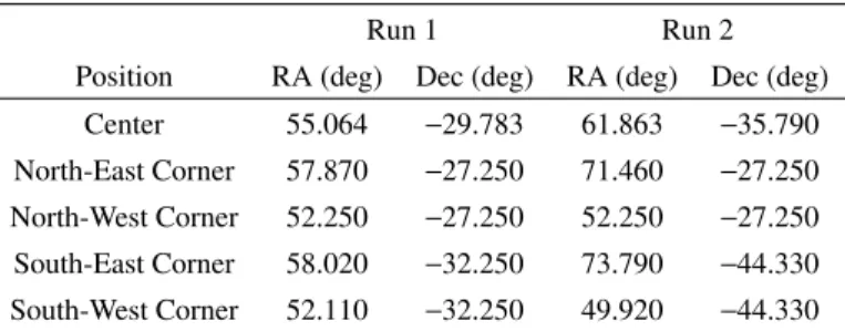
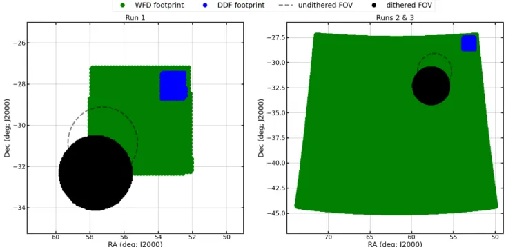
of ∼ 17 degrees;Table 3lists the coordinates for the corners of the WFD region for Run 1 and Run 2. The south-east ex-tension specifies a region that is typical of the planned LSST WFD survey, avoiding low Galactic latitudes and yielding uniform coverage. We show the WFD and DDF regions for all three runs inFigure 2.
Before extracting the visits to simulate, we implement dithers, i.e., telescope-pointing offsets, as they significantly improve the depth uniformity of LSST data, as shown in
Awan et al. (2016). Since dithers are not implemented in
the OpSim runs, we post-process the OpSim output using the LSST Metric Analysis Framework (MAF; Jones et al. 2015) to produce both translational and rotational dithers – which is feasible as each OpSim output contains realizations of the LSST metadata, including telescope pointing and time and filter of observations. The WFD translational dithers and WFD/DDF rotational dithers were implemented using a MAF afterburner10, which post-processed the baseline
ca-dence and added the dithered pointing information to the database. Once the DDF translational dither strategy was
8 docushare.lsst.org/docushare/dsweb/View/Collection-4604
9 A great circle is the intersection between a sphere and a plane through the
center of the sphere. The WFD region simulated here is bounded on the top and bottom by great circles since we use healpy.query routine to connect the four corners of the region; the healpy routine considers all polygons to be spherical polygons.
10github.com/humnaawan/sims_operations/blob/master/tools/schema_tools/ prep_opsim.py
Table 2. Coordinates (J2000) for the simulated DDF.
Position RA (deg) Dec (deg)
Center 53.125 −28.100
North-East Corner 53.764 −27.533 North-West Corner 52.486 −27.533 South-East Corner 53.771 −28.667 South-West Corner 52.479 −28.667 NOTE— DDF coordinates are the same for
Runs 1 and 3.
Table 3. Coordinates (J2000) for the simulated WFD region.
Run 1 Run 2
Position RA (deg) Dec (deg) RA (deg) Dec (deg)
Center 55.064 −29.783 61.863 −35.790
North-East Corner 57.870 −27.250 71.460 −27.250 North-West Corner 52.250 −27.250 52.250 −27.250 South-East Corner 58.020 −32.250 73.790 −44.330 South-West Corner 52.110 −32.250 49.920 −44.330
finalized, we post-processed the afterburner output using a MAF Stacker to implement it for the DDF visits11.
For the WFD region, we implement large translational dithers, i.e., as large as the LSSTCam FOV. Specifically, we use random translational dithers, which have a uniformly ran-dom amplitude in the range [0, 1.75] degrees and a uniformly random direction, applied to every visit; this strategy is based on findings inAwan et al.(2016). For the rotational dithers, we use random offsets from the nominal (LSST OpSim de-fined) camera rotation angle between ± 90 degrees, imple-mented after every filter change.
For the DDF, we implement small translational dithers, i.e., half of the ∼ 7 arcmin angle subtended by an LSSTCam CCD. This is sufficient to mitigate chip-scale non-uniformity and is applied to every visit. We use the same rotational dithering strategy as for WFD: random offsets from the nom-inal rotation angle between ± 90 degrees, applied after every filter change.
For both the WFD and DDF regions, we keep the visits at the same cadence as simulated in the baseline and simply ex-tract the visits that fall within our regions of interest. Note that due to the translational dithers, many visits fall only
par-11github.com/LSSTDESC/DC2_visitList/blob/master/DC2visitGen/ notebooks/DESC_Dithers.ipynb
Figure 2. DC2 footprints showing the WFD region (green) and the simulated DDF (blue). As an illustration, we show a visit (OpSim visit ID 2343 to field 1297 in the u-band filter), in both the pre-processed undithered version (dashed) and the implemented dithered one (filled). Left: Run 1 footprint (WFD and DDF region of the engineering run). Right: Run 2 (WFD region for the science-grade run) and Run 3 footprints (DDF region for the science-grade run).
tially in the region of interest. All of the code for the visit-list generation is in the LSST DESC GitHub repository12.
4. END-TO-END WORKFLOW
The generation of a simulated dataset that resembles the observational data from the LSST requires a complex work-flow that starts with a first-principles structure formation sim-ulation and results in a set of fully processed measurements.
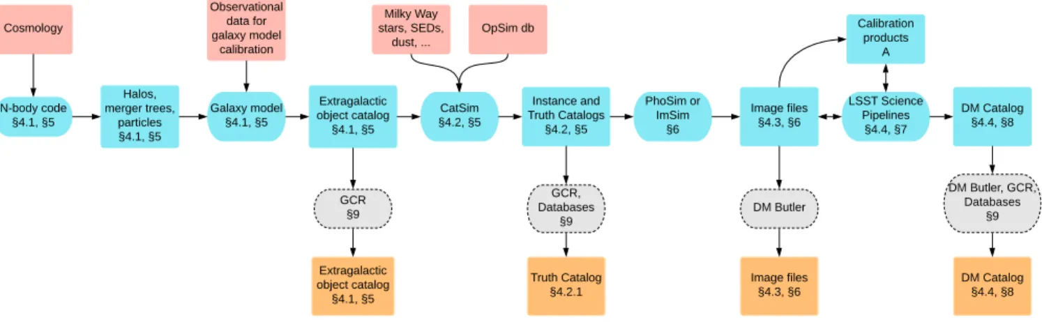
Figure 3provides an overview of the different elements in the
workflow as well as data products that are generated at dif-ferent steps and released to the collaboration. The workflow broadly splits up into four main components: 1) the gener-ation of the extragalactic catalog, 2) the cregener-ation of the in-put catalogs for the image simulations, 3) the image simula-tions themselves, and 4) the processing of the images with the LSST Science Pipelines. Each of these components results in data products that are used in scientific projects. We discuss the four parts of the workflow briefly in the following. After the broad overview has been provided, we dedicateSection 5
to the extragalactic and input catalog generation,Section 6to the image simulations,Section 7to the image processing and
Section 8andSection 9to the data products and access. We
provide the relevant section numbers in each box inFigure 3
to enable easy orientation when navigating the paper. 4.1. The Extragalactic Catalog
The first part of the workflow is based on large cosmologi-cal simulations, carried out using major High-Performance
12github.com/LSSTDESC/DC2_visitList
Computing (HPC) resources. For Run 1, we generated a small extragalactic catalog covering ≈ 25 deg2out to z = 1, called protoDC2. protoDC2 is based on a small simulation (“AlphaQ”), carried out with the Hardware/Hybrid Acceler-ated Cosmology Code (HACC) (Habib et al. 2016) on Coo-ley, a GPU-enhanced cluster hosted at the Argonne Lead-ership Computing Facility (ALCF). The AlphaQ simulation has the same cosmology and approximately the same mass and force resolution as the main simulation used for DC2, Runs 2 and 3, but covers a volume 1600× smaller. This downscaled choice allows for easy handling of the resulting data and many fast iterations to develop and debug the tools needed to create the final catalog.
The main “Outer Rim” simulation was carried out with HACC on Mira, an IBM/BlueGeneQ system that was hosted at the ALCF until the end of 2019. This simulation covers a (4.225Gpc)3volume and evolved more than one trillion par-ticles, resulting in a particle mass of mp= 2.6 · 109M .
De-tails about the simulation are given inHeitmann et al.(2019). From the simulation, halo and particle lightcones were cre-ated and used to generate an extensive extragalactic object catalog called cosmoDC2. A very detailed description of the modeling approach and workflow development is given
inKorytov et al.(2019) and additional information about the
validation process will be published in a forthcoming paper.
InSection 5we provide a brief summary of the catalog
con-tent most relevant for the DC2 production. Access to cos-moDC2 is provided by the Generic Catalog Reader (GCR) which is described in more detail inSection 9.2.
Cosmology Observational data for galaxy model calibration Milky Way stars, SEDs, dust, ... OpSim db N-body code §4.1, §5 Halos, merger trees, particles §4.1, §5 Galaxy model §4.1, §5 Extragalactic object catalog §4.1, §5 CatSim §4.2, §5 Instance and Truth Catalogs §4.2, §5 PhoSim or ImSim §6 Image files §4.3, §6 LSST Science Pipelines §4.4, §7 DM Catalog §4.4, §8 Calibration products A DM Butler Image files §4.3, §6 DM Catalog §4.4, §8 GCR §9 Extragalactic object catalog §4.1, §5 GCR, Databases §9 Truth Catalog §4.2.1 DM Butler, GCR, Databases §9
Figure 3. Workflow overview: The first row (red) shows external inputs to our workflow, which are both physics and modeling parameters, external datasets, or calibration products. The second row (blue) shows the main workflow and intermediate data products. Overall, the workflow breaks up into four pieces: generation of the extragalactic object catalog, generation of the instance and truth catalogs, generation of the image files, and finally generation of the DM catalog. The last two steps also involve the generation of calibration products which can be derived either from the full image simulations or via specific, additional image simulations. In gray, we show different access tools for interacting with the final data products that are shown in orange. Rectangles show input, output or intermediate data products, while ovals represent codes or access methods. In each box we provide the relevant pointers to the sections that describe the specific part of the workflow.
4.2. The Instance Catalogs
The second step in the workflow concerns the generation of the input catalogs to the image simulation tools. The image simulator takes as input a series of “instance catalogs”. An instance catalog is a catalog representing the astrophysical sources whose coordinates are within the footprint of a sin-gle field of view at a sinsin-gle time, a concept originating from the image simulation tool PhoSim (Peterson et al. 2015). Pro-ducing a separate catalog for each simulated telescope point-ing allows us to correctly inject astrophysical variability into the otherwise static cosmological simulation. This is also the step at which extinction due to Galactic dust and astromet-ric shifts due to the motion of the Earth are added to each astrophysical source.
This part of the workflow is enabled by the LSST soft-ware framework CatSim (Connolly et al. 2010,2014). Cat-Sim provides access to a range of LSST specific data, includ-ing position on the LSSTCam focal plane, geocentric appar-ent position, luminosity distance, E(B-V) from Milky Way dust, Av from Milky Way dust, LSST/SDSS (Sloan Digital
Sky Survey) magnitudes/fluxes and uncertainty estimates. In addition, during this step, variability is added to the catalog as well as some galaxy features not readily available from the extragalactic catalog. The outputs of the second step in the workflow are 1) a set of instance catalogs, used as input to the image simulations and 2) truth catalogs that can be accessed via GCRCatalogs or the PostgreSQL Database (Section 9.2
andSection 9.3). For DC2, CatSim was optimized to allow
the creation of a large number of instance catalogs in a short amount of time. We impose a cut on galaxies from the cos-moDC2 catalog with magnitudes larger than 29 in r-band to reduce the catalog sizes, retaining ∼ 42% of the galaxies. Since version 19.0.0 of the LSST Science Pipelines, which
we used for image processing, cannot handle proper motion and parallax of stars, we omitted those effects from the in-stance catalog entries for those objects.
4.2.1. The Truth Catalogs
In order to verify that the inputs to the image simulations, i.e., the instance catalogs, are correct and to assess the fi-delity of the output catalogs that are produced by the im-age processing, we have generated “truth catalogs” based on our model of the sky. These catalogs contain the true values of the measurable properties of objects as produced by the LSST Science Pipelines software. As we describe in
Sec-tion 7, the image processing outputs comprise catalogs of
objects detected and identified in the coadded observations, with measured positions, fluxes, and shape parameters pro-vided for each object. Catalogs of measured fluxes are also produced for each visit in order to characterize time vari-ability. Accordingly, our truth catalogs include two tables: a summary truth table that captures the time-averaged prop-erties of objects and a variability truth table that provides for each visit an object’s flux with respect to the time-averaged value. The procedure for assessing the fidelity of the LSST Science Pipelines outputs is then straightforward: After per-forming a positional match between truth catalog objects and the LSST catalog objects, the differences between true and measured fluxes and between the true and measured posi-tions can be examined and compared to the expected levels of photometric and astrometric accuracy and precision. We introduced our matching procedure inSánchez et al.(2020). First, a positional query between the true objects and de-tected objects is carried out. Next, we consider sources in the object catalog as “matched" if there is a source in the true catalog that is within one magnitude of the measured mag-nitude in r-band (we use r-band because it is the deepest).
Using this procedure blended objects will still be matched if the deblender performed reasonably well and we eliminate problematic sources that have been shredded. In some cases two or more sources of similar surface brightness are blended and have been detected as just one source. Those will not be considered as matches but we still provide the closest neigh-bor. The radius for the position matching was chosen to be 100. This yielded a good compromise between accuracy and speed.
For the verification of the instance catalogs, the procedure is different and somewhat more complicated. One key differ-ence between the truth table flux values and the information in the instance catalogs is that the truth tables provide the fluxes integrated over each bandpass, including any internal reddening, redshift, Milky Way extinction, and the effects of atmospheric and instrumental throughputs. These fluxes are the “true” values that would be measured for isolated objects with infinite signal-to-noise ratio. By contrast, the instance catalog entry for an object component provides a tabulated SED, the monochromatic magnitude at 500 nm, the redshift, and internal and Milky Way extinction parameters. As we de-scribe inSection 6, the image simulation code arrives at the flux for each object by applying each of the ingredients in the instance catalog description in turn. For PhoSim, this is ac-complished by drawing individual photons from the normal-ized SED and tracing their paths through each element of the simulation. For imSim/GalSim, the fluxes are computed by direct integration over the observed bandpasses. For galax-ies, another important difference between the summary truth tables and the instance catalogs is that the summary truth ta-bles combine the fluxes from the bulge, disk, and knot com-ponents, thereby producing a single entry for each galaxy as a whole, whereas the instance catalogs provide separate entries for each of the three possible galaxy components. Therefore, to verify an instance catalog, those integrations over band-passes are computed and the sum over contributions from each galaxy component is made. Since we have object IDs for the truth and instance catalog entries that allow objects to be matched definitively, positional matching is not needed, and the truth and instance catalog fluxes can be compared di-rectly. We expect those values to agree to machine precision and verified that this is indeed the case.
4.3. The Image Simulations
The instance catalogs, now containing information about galaxies, stars, the Milky Way, observing conditions and so on, are processed next by image simulation tools. This step delivers simulated pixel data from the LSST focal plane and is described in detail inSection 6. For Run 1, we em-ployed two image simulation tools, PhoSim (Peterson et al. 2015) and imSim (DESC, in preparation). We used the pro-toDC2 catalog as input for both runs and carried out the PhoSim image simulations (using subversions of v3.7) at the National Energy Research Scientific Computing Center (NERSC) with the SRS Workflow setup (Flath et al. 2009). The SRS workflow engine was also used for the processing of the image simulations and is briefly described inSection 7.2.
Run 1 with imSim (v0.2.0-alpha) was carried out on Theta at the ALCF, a Cray XC40 with Intel Knights Landing (KNL) processors. We used a Python-based script to define the over-all workload, manage submission and monitoring of jobs, and to validate output images, in an iterative fashion, on up to 2,000 nodes; a great majority of these runs were completed over a long weekend. This run was done after the PhoSim run, using the instance catalogs that had been generated al-ready.
For the final DC2 image data, we divided the simulations into two separate runs, Run 2 and Run 3. Run 2 includes all of the minion_1016 visits and covers the entire 300 deg2,
but since these data would be used primarily by the static dark energy probes (weak lensing, large-scale structure, clus-ters) that do not rely on the analysis of time-varying objects, we omitted the AGN at the centers of galaxies, although we do include ordinary SNe and variable stars, as well as non-varying stars, as these latter objects are needed for perform-ing the astrometric and photometric calibration for the image processing. By contrast, Run 3 is designed specifically for the time domain probes, SNe and strong lensing cosmogra-phy. It just covers the DDF region and includes the time-varying objects, i.e., the ordinary AGN and SNe, the strongly lensed AGN and SNe, as well as the strongly lensed hosts for those objects. Since the non-varying sky for the DDF re-gions comprises the same static scenes that were produced in Run 2, in order to save computing resources, we rendered the additional strongly lensed and time-varying objects on top of the Run 2 images, doing so before applying the elec-tronic readout so that the instrumental effects would be simu-lated consistently. In the following we will use the shorthand Run 2/3 whenever the full set of DC2 image simulations is discussed.
Due to limited resources, for the Run 2/3 simulations, we employed only imSim (Run 2 simulations were carried out with imSim v0.6.2 and Run 3 with v1.0.0). The decision to use imSim for the main run was made after carefully evalu-ating the results from the engineering runs with PhoSim and imSim, including the results from a range of validation tests, and performance when comparing the two codes using set-tings that met the validation criteria. The conclusion was that the setup chosen for Run 2/3 would permit the production of simulations that would enable the science goals outlined
inSection 2within the available human and computing
re-sources.
A new workflow setup was developed based on Parsl (Babuji et al. 2019) to allow scaling up the simulation campaigns to thousands of nodes. The workflow implemen-tation is described in detail inSection 6.2. Run 2 was carried out on Cori, a KNL architecture-based system at NERSC and on grid resources in the UK and France; Run 3 was carried out on Theta. Overall, Run 2/3 generated just under 100TB of simulated image data.
4.4. The Image Processing
Finally, in the fourth step, the data is processed with the LSST Science Pipelines. For all three runs, the
process-ing was carried out at the Centre De Calcul – Institut Na-tional de Physique Nucléaire et de Physique des Particules du CNRS (CC-IN2P3) using an SRS-based workflow setup. Since Run 2 consists predominately of WFD observations, the processing of the data is limited to the analysis of the coadded images. The results from coadd processing com-prise the catalog outputs needed by the weak lensing, large-scale structure, and clusters dark energy probes. By contrast, for the Run 3 data, we will focus on the difference image analysis (DIA) processing13since the purpose of Run 3 is the
simulation of the time varying objects that are needed by the supernova and strong lensing probes.
We could, in principle, perform the coadd and DIA pro-cessing for both Run 2 and Run 3, but Run 2 lacks those time varying objects, thereby making its DIA processing of lim-ited value, and the much greater numbers of visits for the DDF (roughly 2 orders of magnitude more visits than for non-DDF regions) make it too computationally costly to jus-tify the full coadd processing of the data in the vicinity of the DDF for either Run 2 or Run 3. Specifically, for the Run 2 data, we exclude from the coadd processing tracts and patches14that enclose regions with > 4000 seconds exposure
time in the i-band. We note that the DIA processing is the subject of ongoing work and will be presented in a future paper.
During the image processing, intermediate and final data products were generated at the scale of 1PB. Approximately 80% of those data products consist of calibrated single-visit exposures, versions of those exposures that have been resam-pled onto a common pixelization on the sky, and coadded images in each band, which were generated from the resam-pled visit-level frames. The final object catalogs added up to less than 2.5TB of data. The image processing for all three runs is described in detail inSection 7.
In the following we provide an extensive description of the modeling approaches, codes and workflows used in each of the four key steps of survey generation as well as of the re-sulting data products.
5. MODELING THE DC2 UNIVERSE
In this section we describe the first and the second step of our end-to-end workflow, i.e., the generation of the extra-galactic catalog, cosmoDC2, and the additional components of the Universe that are included in the instance catalogs. We divide the description into three parts – the static components of the DC2 Universe, the variable components, and the local DC2 Universe. All three parts are combined via the CatSim framework to create the input to the image simulations.
5.1. The Static DC2 Universe
13See project.lsst.org/meetings/lsst2019/content/ difference-image-analysis-dia-parallel-workshop for a discussion of DIA processing of Rubin Observatory data.
14“Tracts” and “patches” are regions of the sky defined for the image
pro-cessing pipeline. They are described inSection 7.
The cosmoDC2 extragalactic catalog (Korytov et al. 2019) is based on the gravity-only Outer Rim simulation (Heitmann
et al. 2019), which evolved more than a trillion particles in a
(4.225 Gpc)3 volume. CosmoDC2 covers 440 deg2 of sky area to a redshift of z = 3 and is complete to a magnitude depth of 28 in the LSST r-band. The sky area of cosmoDC2, which is delivered in HEALPix15 (Hierarchical Equal Area
iso-Latitude Pixelization) format (Gorski et al. 2005), was chosen so that the predefined image area would be covered. Hence it is slightly larger than DC2 in order to account for edge effects. The catalog also contains many fainter galax-ies to magnitude depths of ≈ 33 for use in weak lensing and blending studies. Faint galaxies with r-band magnitudes > 29 are removed from the image simulations to reduce the number of objects that need to be rendered (seeSection 4.2). The catalog is produced by means of a new two-step hy-brid method that combines empirical modeling with the re-sults from semi-analytic model (SAM) simulations. In this approach, the Outer Rim halo lightcone is populated with galaxies according to an empirical model that has been tuned to observational data such that the distributions of a restricted set of fundamental galaxy properties consisting of positions, stellar masses and star-formation rates are in good agreement with a variety of observations (Korytov et al. 2019;Behroozi
et al. 2019). Additional modeling for the distributions of
LSST r-band rest-frame magnitude and g − r and r − i colors is also done in this step. These properties are not sufficient for performing the image simulations, most notably since observer-frame magnitudes have not yet been specified. In order to provide a full complement of galaxy properties, we invoke the second step in the hybrid approach. The galaxies from the empirical model are matched with those from the SAM by performing a KDE-Tree match on the rest-frame magnitude and colors. These matched SAM galaxies now provide all the required galaxy properties including morphol-ogy, SEDs, and broadband colors. The properties are self-consistent, incorporate the highly nonlinear relationships that are built into the SAM and capture some of the complexity inherent in the real Universe. In our hybrid method, the SAM galaxies function as a galaxy library from which to draw a suitable subset of galaxies that match observations and have the complex ensemble of properties that are required by DC2. The method is predicated on the assumption that the proper-ties that have been tuned in the empirical model are suffi-ciently correlated with the other properties obtained from the SAM library to ensure that the latter will also be realistically distributed.
The empirical model used for cosmoDC2 is based on Uni-verseMachine (Behroozi et al. 2019), augmented with addi-tional rest-frame magnitude and color modeling. This model is applied to Outer Rim halos to populate its halo light-cone with galaxies. Then, as described above, these galax-ies are matched to those that have been obtained by run-ning the Galacticus SAM (Benson 2012) on the small