Measurement of pion and proton response and longitudinal shower profiles up to 20 nuclear interaction lengths with the ATLAS Tile calorimeter

CERN-PH-EP-2009-019

CERN-PH-EP/2009-019

8 October 2009

Measurement of Pion and Proton Response and

Longitudinal Shower Profiles up to 20 Nuclear

Interaction Lengths with the ATLAS Tile Calorimeter

P. Adragnaa_{, C. Alexa}b_{, K. Anderson}c_{, A. Antonaki}d_{, A. Arabidze}d_, L. Batkovae_{, V. Batusov}f_{, H. P. Beck}g_{, E. Bergeaas Kuutmann}h_{, C. Biscarat}i_,

G. Blanchotm_{, A. Bogush}k_{, C. Bohm}h_{, V. Boldea}b_{, M. Bosman}j_, C. Brombergl_{, J. Budagov}f_{, D. Burckhart-Chromek}m_{, M. Caprini}b_, L. Caloban_{, D. Calvet}i_{, T. Carli}m_{, J. Carvalho}o_{, M. Cascella}a_{, J. Castelo}p_,

M. V. Castillop_{, M. Cavalli-Sforza}j_{, V. Cavasinni}a_{, A. S. Cerqueira}n_, C. Clementh_{, M. Cobal}m_{, F. Cogswell}q_{, S. Constantinescu}b_{, D. Costanzo}a_, A. Corso-Radum_{, C. Cuenca}p_{, D. O. Damazio}n_{, T. Davidek}s,m_{, K. De}t_{, T. Del}

Pretea_{, B. Di Girolamo}m_{, S. Dita}b_{, T. Djobava}u_{, M. Dobson}m_{, J. Novakova}s_, A. Dottia_{, R. Downing}q_{, I. Efthymiopoulos}m_{, D. Eriksson}h_{, D. Errede}q_, S. Erredeq_{, A. Farbin}t_{, D. Fassouliotis}d_{, R. Febbraro}i_{, A. Fenyuk}v_{, C. Ferdi}i_,

A. Ferrerp_{, V. Flaminio}a_{, D. Francis}m_{, E. Fullana}p_{, S. Gadomski}g_, S. Gameirom_{, V. Garde}i_{, K. Gellerstedt}h_{, V. Giakoumopoulou}d_, O. Gildemeisterm_{, V. Gilewsky}w_{, N. Giokaris}d_{, N. Gollub}m_{, A. Gomes}r_, V. Gonzalezp_{, B. Gorini}m_{, P. Grenier}m,i_{, P. Gris}i_{, M. Gruwe}m_{, V. Guarino}x_,

C. Guicheneyi_{, A. Gupta}c_{, C. Haeberli}g_{, H. Hakobyan}y_{, M. Haney}q_, S. Hellmanh_{, A. Henriques}m_{, E. Higon}p_{, S. Holmgren}h_{, M. Hurwitz}c_, J. Hustonl_{, C. Iglesias}j_{, A. Isaev}v_{, I. Jen-La Plante}c_{, K. Jon-And}h_{, M. Joos}m_,

T. Junkq_{, A. Karyukhin}v_{, A. Kazarov}z_{, H. Khandanyan}q_{, J. Khramov}f_, J. Khubuau,f_{, S. Kolos}z_{, I. Korolkov}j_{, P. Krivkova}s_{, Y. Kulchitsky}k,f_, Yu. Kurochkink_{, P. Kuzhir}w_{, T. Le Compte}x_{, R. Lefevre}i_{, G. Lehmann}m_, R. Leitners_{, M. Lembesi}d_{, J. Lesser}h_{, J. Li}t,1_{, M. Liablin}f_{, M. Lokajicek}aa_,

Y. Lomakinf,1_{, A. Lupi}a_{, C. Maidanchik}n_{, A. Maio}r_{, M. Makouski}v_, S. Maliukovf_{, A. Manousakis}d_{, L. Mapelli}m_{, C. Marques}r_{, F. Marroquim}n_, F. Martinm,i_{, E. Mazzoni}a_{, F. Merritt}c_{, A. Miagkov}v_{, R. Miller}l_{, I. Minashvili}f_,

L. Mirallesj_{, G. Montarou}i_{, M. Mosidze}u_{, A. Myagkov}v_{, S. Nemecek}aa_, M. Nessim_{, L. Nodulman}x_{, B. Nordkvist}h_{, O. Norniella}j_{, A. Onofre}ab_, M. Oregliac_{, D. Pallin}i_{, D. Pantea}b_{, J. Petersen}m_{, J. Pilcher}c_{, J. Pina}r_, J. Pinh˜aoo_{, F. Podlyski}i_{, X. Portell}j_{, J. Poveda}p_{, L. Pribyl}aa,m_{, L. E. Price}x_,

J. Proudfootx_{, M. Ramstedt}h_{, R. Richards}l_{, C. Roda}a_{, V. Romanov}f_, P. Rosneti_{, P. Roy}i_{, A. Ruiz}p_{, V. Rumiantsev}w,1_{, N. Russakovich}f_{, O. Salt´o}j_, B. Salvachuap_{, E. Sanchis}p_{, H. Sanders}c_{, C. Santoni}i_{, J. G. Saraiva}r_{, F. Sarri}a_,

I. Satsunkevitchk_{, L.-P. Says}i_{, G. Schlager}m_{, J. Schlereth}x_{, J. M. Seixas}n_, B. Selld`enh_{, N. Shalanda}v_{, P. Shevtsov}w_{, M. Shochet}c_{, J. Silva}r_{, P. Da Silva}n_,

V. Simaitisq_{, M. Simonyan}y_{, A. Sissakian}f_{, J. Sj¨olin}h_{, C. Solans}p_, A. Solodkovv_{, I. Soloviev}z_{, O. Solovyanov}v_{, M. Sosebee}t_{, F. Span`o}ad_,

1

R. Stanekx_{, E. Starchenko}v_{, P. Starovoitov}w_{, P. Stavina}e_{, M. Suk}s_{, I. Sykora}e_, F. Tangc_{, P. Tas}s_{, R. Teuscher}c_{, S. Tokar}e_{, N. Topilin}f_{, J. Torres}p_, L. Trembletm_{, P. Tsiareshka}f,k_{, M. Tylmad}h_{, D. Underwood}x_{, G. Unel}m,ac_, G. Usaia_{, A. Valero}p_{, S. Valkar}s_{, J. A. Valls}p_{, A. Vartapetian}t_{, F. Vazeille}i_, I. Vichouq_{, V. Vinogradov}f_{, I. Vivarelli}a_{, M. Volpi}j_{, A. White}t_{, A. Zaitsev}v_,

A. Zeninev_{, T. Zenis}e

a_{Pisa University and INFN, Pisa, Italy}

b_{National Institute for Physics and Nuclear Engineering, Bucharest, Romania} c_{University of Chicago, Chicago, Illinois, USA}

d_{University of Athens, Athens, Greece} e_{Comenius University, Bratislava, Slovakia}

f_{JINR, Dubna, Russia}

g_{Laboratory for High Energy Physics, University of Bern, Switzerland} h_{Stockholm University, Stockholm, Sweden}

i_{LPC Clermont–Ferrand, Universit´e Blaise Pascal, Clermont-Ferrand, France} j_{Institut de Fisica d’Altes Energies, Universitat Aut`onoma de Barcelona, Barcelona, Spain}

k_{Institute of Physics, National Academy of Sciences, Minsk, Belarus} l_{Michigan State University, East Lansing, Michigan, USA}

m_{CERN, Geneva, Switzerland} n_{COPPE/EE/UFRJ, Rio de Janeiro, Brazil} o_{LIP and FCTUC Univ. of Coimbra, Portugal}

p_{IFIC, Centro Mixto Universidad de Valencia-CSIC, E46100 Burjassot, Valencia, Spain} q_{University of Illinois, Urbana–Champaign, Illinois, USA}

r_{LIP and FCUL Univ. of Lisbon, Portugal}

s_{Charles University, Faculty of Mathematics and Physics, Prague, Czech Republic} t_{University of Texas at Arlington, Arlington, Texas, USA}

u_{HEPI, Tbilisi State University, Tbilisi, Georgia} v_{Institute for High Energy Physics, Protvino, Russia}

w_{National Centre of Particles and High Energy Physics, Minsk, Belarus} x_{Argonne National Laboratory, Argonne, Illinois, USA}

y_{Yerevan Physics Institute, Yerevan, Armenia}

z_{Petersburg Nuclear Physics Institute (PNPI), Gatchina, Russia}

aa_{Institute of Physics, Academy of Sciences of the Czech Republic, Prague, Czech Republic} ab_{LIP and Univ. Cat´olica Figueira da Foz, Portugal}

ac_{University of California, Irvine, CA 92717, USA}

ad_{Columbia University, Nevis Laboratories, Irvington, NY 10533, USA}

Abstract

The response of pions and protons in the energy range of 20 to 180 GeV produced at CERN’s SPS H8 test beam line in the ATLAS iron-scintillator Tile hadron calorimeter has been measured. The test-beam configuration allowed to mea-sure the longitudinal shower development for pions and protons up to 20 nuclear interaction lengths. It is found that pions penetrate deeper in the calorimeter than protons. However, protons induce showers that are wider laterally to the direction of the impinging particle. Including the measured total energy re-sponse, the pion to proton energy ratio and the resolution, all observations are consistent with a higher electromagnetic energy fraction in pion induced show-ers. The data are compared with GEANT4 simulations using several hadronic

physics lists. The measured longitudinal shower profiles are described by an analytical shower parameterization within an accuracy of 5 − 10%. The amount of energy leaking out behind the calorimeter is determined and parameterised as a function of the beam energy and the calorimeter depth. This allows for a leakage correction of test-beam results in the standard projective geometry.

Introduction

The Large Hadron Collider (LHC) at CERN collides protons with an energy of 7 TeV. The resulting high center of mass energy will open a new chapter for particle physics exploring the high energy frontier.

Hadronic calorimeters have the main task to measure the energy and direc-tions of jets, sprays of hadrons of various species that emerge from the hard parton–parton scattering. Their hermeticity allows, in addition, to measure the missing transverse energy and therefore to partly reconstruct particles that are escaping detection. The understanding of the calorimeter response to hadrons and of their shower development is crucial to achieve the best possible perfor-mance of the energy measurement.

While usually the calorimeter response is tested using single pions test-beams, in the colliding beam experiment, jets are measured. Differences in the response of pions, kaons, protons and neutrons (and the corresponding anti-particles and other rare mesons and hadrons) are assumed to be small or de-scribed by the Monte Carlo simulation.

In 1994, however, it was pointed out that the response of non-compensating calorimeters to pions and protons can be slightly different [1], since the under-lying production mechanism of the first few interactions of the hadron in the calorimeter is different. Based on Monte Carlo simulations a phenomenological model was developed that predicted the same energy depositions of hadronic nature for pions and protons, but more electromagnetic energy depositions and larger fluctuations in the electromagnetic energy fraction in the case of pions. These effects were experimentally confirmed in 1998 [2,3].

Here, we study the response of the Tile Calorimeter (TileCal), located in the barrel part of the ATLAS detector, to pions and protons in the energy range of 20 to 180 GeV produced at the CERN SPS H8 test beam line. The data have been taken in the year 2002. The calorimeter response, the resolution and the longitudinal and lateral shower development is studied for pions and protons.

The TileCal consists of steel plates used as absorber material and scintillating tiles used as active medium. The new feature of the TileCal design is the orientation of the scintillating tiles which are placed in planes perpendicular to the colliding beams. However, for the runs analyzed here a special non-projective configuration of the test beam set-up has been used where the beam direction is perpendicular to the scintillating tiles (“90 degree configuration”). This configuration allows almost full shower containment and makes it possible to measure shower profiles up to 20 nuclear interaction lengths1 _(λ).

Previously, in the energy range of 10 - 140 GeV the longitudinal shower pro-files for an iron-scintillator structure have been studied for the CDHS calorime-ter [4], which had alternating scintillator and irons layers of 5 mm and 25 mm (compared to 3 mm and 14 mm in TileCal) and whose readout cells consisted

1

Throughout this analysis an effective nuclear interaction length for the Tile calorimeter is used. The value is λ = 20.55 cm, calculated using the known fraction of materials used in the detector construction and their nuclear interaction lengths.

of 5 scintillator-iron layers, whereas the typical TileCal readout cells was about 30 cm twice as long. The CDHS calorimeter was 240 cm long in the beam direction, to be compared to 564 cm for the TileCal Barrel modules in the 90 degree configuration. In a recent publication of the TileCal collaboration the longitudinal shower profile has been measured for prototype modules2_{, having}

a depth of 180 cm (9 λ) and coarse granularity [5].

The results are also compared to Monte-Carlo (MC) simulations using several hadronic physics models available in the GEANT4 [6] framework. The detailed measurements contribute to test existing simulation packages and to guide their future development such that the stringent requirements to correctly model the calorimeter response, and in particular the hadronic shower development, imposed by the LHC physics programs, can be reached.

The paper is organized as follows:

In Section1, the TileCal test beam set-up together with the beam line detec-tors are briefly described. The Monte Carlo simulation including the various hadronic interaction models are described in Section 2. The data-set and the event selection is presented in Section3. and particle identification in Section4. In Section5the reconstruction of the hadron energy is briefly reviewed and the uncertainty in the energy measurement are discussed. In Section 6 the mea-surements of the response, the resolution, the longitudinal shower profile and the lateral shower spread are presented and in Section7they are compared to Monte Carlo simulations.

Section8 presents a phenomenological interpretation of the data. The elec-tromagnetic fraction contained in pion and proton induced showers is extracted and an analytical parameterization to describe the mean longitudinal shower profile is presented. Special emphasis is put on differences between protons and pions. The results obtained using the TileCal in this analysis are compared to measurements with the CDHS calorimeter and with TileCal proto-types mod-ules in Section9. Based on the analytical parameterization of the shower profile a determination of the mean longitudinal leakage is presented in Section10. In this section the mean longitudinal leakage is also compared to the longitudinal leakage defined as the shift of the peak of the total energy distribution obtained from a Gaussian fit. The energy and angular dependence of the longitudinal leakage is determined and parameterized. In addition, the energy resolution as a function of the calorimeter depth is presented.

2

These measurements have been performed in projective geometry. This means that the particles enter the calorimeter as they would do in the ATLAS detector, if they were produced at the proton proton interaction point.

0.1 0.2 0.3 0.4 0.5 0.6 0.7 0.8 0.9 1.0 D BC A 0.8 0.9 1.0 1.1 1.2 1.3 1.4 1.5 1.7 1.6 Tile Calorimeter

Cells and Tile Rows

Half-Barrel Extended Barrel

0 500 1500 mm D0 D1 D2 D3 BC1 BC2 BC3 BC4 BC5 BC6 BC7 BC8 B9 A1 A2 A3 A4 A5 A6 A7 A8 A9 A10 D5 D4 D6 B11 B12 B13 B14 B15

A A13 A14 A15 A16 C

1

1000

0

12

Figure 1: Sketch of the cell granularity of a TileCal module. The line indicate the direction of particles produced at the nominal vertex in the ATLAS detector.

1. Experimental Set-up 1.1. The Tile Barrel Calorimeter

The iron-scintillator media of the TileCal modules is made of 4 mm and 5 mm thick iron plates sandwiched by 3 mm thick scintillator tiles, with a periodicity of 18 mm. The total thickness of the iron and the scintillator in a period is 14 mm and 3 mm, respectively. The tiles are oriented perpendicularly to the modules length such that the Barrel Module is extended over 307 periods. Each side of the scintillating tiles is readout by a single wave length shifting (WLS) fiber. The fibers are grouped together, separately for each side, forming a cell, that is readout by two photo-multipliers (PMT).

Each TileCal module is one of 64 azimuthal segments of the complete Barrel and Extended Barrel assembly of the Tile calorimeter in ATLAS (see for details [7]). The module design was driven by the requirement of productivity in the η-plane3_{and in the radial direction (φ). The TileCal has a granularity of cells}

spanning ∆η = 0.1 and ∆φ = 2π/64 = 0.1. Eleven tile sizes are used in the structure of the Barrel Modules, grouped into the clusters of 3+6+2 tiles, defining three radial samplings A, BC and D with depths of 1.5, 4.1 and 1.9 λ at η = 0, respectively. A sketch of the cell granularity in a TileCal module is shown in Fig.1.

The scintillating light produced in the tiles is transported via wavelength shifting fibres into photo-multipliers (PMT). The PMTs amplify the signal and convert the optical signal into an electrical one. Each PMT channel has two analogue paths: the high and the low gain with 82 cts/pC and 1.3 cts/pC. The

3

The η and φ directions are chosen with respect to a reference frame with cylindrical coordinates having its origin in the virtual proton-proton interaction point in ATLAS. In this coordinate system the z-axis is defined along the beam axis. The φ and θ angles are the azimuthal and polar angles. The pseudo-rapidity is defined by η = − log tan θ/2.

−90

+90

+20

Figure 2: Configuration of the calorimeter modules in the test beam set-up. The arrows indicate the direction of the impinging particles. In this analysis runs are used where the beam hit TileCal from the side (called 90o_{). In ATLAS and in the standard test-beam configuration}

the beam impinges under a smaller angle. An angle of 20o _{is indicated as example.}

read-out electronics shapes, amplifies and digitizes the signals from the PMTs. The shaped signals are sampled every 25 ns by a 10-bit ADC.

1.2. Test Beam Set-up and Beam Line Detectors

The H8 test beam line at the SPS accelerator of CERN is instrumented with a set of beam detectors: scintillator trigger counters (S1-S3), wire chambers (BC1-BC2) measuring the lateral x and y position of the beam particles and a helium filled threshold Cherenkov counter. The scanning table carrying the modules was used to reproduce the angles of incidence of particles originating from the LHC interaction region (see Fig.1).

The layout of the TileCal modules in the H8 test beam line area is shown in Fig.2. It consists of one production Barrel Module, 5.64 m long, two production modules of the Extended Barrel, 2.93 m long, which are stacked together on top of the prototype Barrel Module 0.

The beam energy has been precisely determined for each run using the mea-sured currents in the bending magnets and the collimator setting. The exact numbers together with the nominal beam energy are given in Tab.2.

The Extended Barrel modules are not used in the measurement of the lon-gitudinal shower profile due to the difficulty of accounting for the large gap (equivalent to two barrel layers) between two modules in the test beam set-up. Instead, the energy measured in the Barrel Module 0 is multiplied by a factor of two4_.

4

Taking into account that the direction of the initial particle is a symmetry axis and the distance from the axis to Module 0 and Extended Barrel module is equal, this procedure measures correctly the mean energy and the average longitudinal shower profile. However, the resolution is made somewhat worse, since event-by-event fluctuations can not be followed.

As indicated in Fig. 2 the beam impinges from the side of the production Barrel Module, perpendicularly to the scintillating tiles. The direction of the beam is defined to be the x-axis. The beam impact point has been chosen to be on the center of the fifth tile row of the BC cell. This choice takes advantage of the relatively fine longitudinal segmentation of the BC cells while giving good lateral containment of the showers, because the distance from the beam axis to the exit of the bottom Module 0 and the top of the EB Module is approximately 2 λ.

Longitudinally showers are fully contained in the calorimeter, since no energy is observed in the last layers of the modules. The lateral containment of the shower in the test beam set-up is about 99% as shown in Section8.1.

2. Monte Carlo Simulation Tools 2.1. Simulation of Hadronic Showers

The simulation of the calorimeter modules was performed within the ATLAS software framework using the GEANT4 simulation toolkits [6].

The Monte Carlo simulation models the interaction of particles with the detector material on a microscopic level. The detailed shower development follows all particles that interact electromagnetically in the calorimeter with an expected travel path (range) larger than 1 mm. Besides purely electromagnetic processes, also hadron interactions and photo-nuclear interactions are simulated. Neutrons are followed in detail up to 10 µsec. After that time all their energy is deposited at the location of the neutron.

The strong interaction of hadrons is modelled in four phases depending on the energy range:

1. The interaction of the projectile with the nucleus using parameterised re-action cross-section for various processes (fission, capture, elastic, inelastic scattering)

2. The fragmentation of the partons produced in the inelastic hadron nucleon collision using theory driven or parameterised models (≈ 10 GeV - 10 TeV) 3. The interactions of the hadrons in the medium of the nucleus are modelled

using intra-nuclear nucleon cascades (1 − 10 GeV).

4. Nuclear processes to de-excited or split the excited nucleus via spallation, break-up, fission etc.(1 − 100 MeV).

Within the GEANT4 simulation framework several models can be used to simulate the interaction of particles with matter. The applicability of the model depends on the particle type, the energy range and the target material. There is also the possibility to use different models for the same particle type and energy range. A “physics list” is a consistent collection of models that covers the interaction of all particles in the whole energy range from thermal energies to the several TeV range. Therefore, depending on the application and on the required physics performance and the available computing time, different physics lists can be chosen.

In this study, four different physics lists have been used which are recom-mended for calorimeter studies at LHC energies.

The physics list LHEP employs parameterization-driven models for all hadronic interactions using measured and extrapolated reaction cross-sections, particle spectra and multiplicities for the final state. Several parameters have been tuned in a global fit to describe a large number of hadron-hadron scattering data. It contains the Low Energy Parameterized (LEP) model for interaction of hadrons for low energies and the High Energy Parameterized (HEP) model for higher energies5_.

As a result, the LHEP physics list provides a fast simulation, but baryon and meson resonances are not produced and the secondary angular distributions for low energy reactions of O(100 MeV) cannot be described in detail. This model is a re-implementation of the GHEISHA model in GEANT3.21 [8].

The second physics list QGSP employs the formalism of the quark-gluon string (QGS) model for soft and fast ’punch-through’ interactions of the projec-tile with nucleons of the nuclear medium. The string excitation cross-sections are calculated in the quasi-eikonal approximation. QGSP uses Barashenkov’s pion cross-section [9] and the Wellisch-Axen systematics for nucleon induced reactions [10]. At low energies QGS is not applicable and the LEP model is used instead6_{. The pre-compound model is used for de-excitation of a nucleus}

left in an excited state after energetic interaction.

In both physics lists, QGSP and LHEP, the Bertini intra-nuclear cascade model for hadron-nucleus interactions can be added (QGSP BERT and LHEP BERT). In this case the strong interaction of hadrons below 10 GeV is simulated accord-ing to the Bertini model [11,12,13]7_{. In this model the projectile and induced}

secondaries are transported along straight lines through the nuclear medium (approximated by concentric, constant-density shells) and interact using the free hadron-nucleon total cross-section. At the shell boundaries a particle can be reflected or transmitted. As cascade collisions occur, excited residual nuclei are formed which can then evaporate neutrons or alpha particles and can ra-diate photons due to inter-nuclear transitions, as well as undergo weak decay with subsequent de-excitation.

2.2. Detector Simulation

The simulation of the TileCal models the detailed structure of the scintillat-ing tiles and the iron absorber.

5

The code applies the HEP (or the LEP) model with a probability that increases from zero to 1 (or decreases from 1 to zero) linearly as the hadron energy increases from 25 GeV to 55 GeV.

6

The QGS (LEP) model is always used for energies above 25 GeV (below 12 GeV). Hadrons between 12 and 25 GeV are treated by either model, with the choice being made event by event by a linearly varying probability.

7

The Bertini model is fully used up to 9.5 GeV. The LEP model is fully used for energies larger than 9.9 GeV. For energies between 9.5 and 9.9 GeV a choice between the two models based on a linearly increasing probability is made.

The simulation of the TileCal scintillators includes saturation effects mod-elled according to Birks law and the effects of statistics in the photo-multipliers. However, no attempt is made to describe the detailed optical prop-erties of the scintillating tiles and the read-out fibres.

Also the light attenuation between the two PMTs is not modelled. A simple linear interpolation is used to distribute the energy to the PMT on each cell side. The maximal drop of the signal between the two PMTs of a cell due to non-linearities is not larger than 5%.

The electronic noise was extracted from experimental data using randomly triggered events and added incoherently to the energy of each PMT in the MC samples. Coherent noise is not simulated, but known to be relatively small [14]. A sample of 10000 events was simulated for each physics list and for each beam energy and particle type.

3. Data Set and Event Selection 3.1. Data Set and Event Selection

The data analyzed here were taken in June and July of the year 2002. The energy range from 20 to 180 GeV is covered.

Events in the tails of the lateral beam profile are eliminated with the help of the beam chambers. The response of the chambers is fitted with a Gaussian and all events within three standard deviations around the mean are accepted. These cuts reduce the momentum spread of the beam and decrease the acceptance for events, where a hadron decays or interacts early in the material of the H8 beam line before entering the calorimeter.

In each of the scintillator counters S1-S3, a signal compatible with the one from a minimum ionizing particle is required in order to remove multiple hits from accidental coincidences of beam particles and to reject early showering hadrons.

The reconstructed time and energy of all PMTs are used to reconstruct the energy weighted event time. All events within three standard deviations around the mean are accepted.

4. Particle Identification

The hadron beams produced at the H8 beam line contain in general a mixture of electrons, muons, pions, protons and possibly also kaons, depending on the beam energy, the used target (primary, secondary or tertiary) and the beam line optics.

It is therefore necessary to identify the type of the particle impinging to the calorimeter and to determine the purity of the selected sample. If possible, external detectors like the Cherenkov counter are used for particle identification. However, it is also necessary to use the information from the calorimeter itself. In this case a bias on the calorimeter measurement is introduced and needs to

be carefully evaluated either by studying the effect of the cut in the data or by using a MC simulation.

It has been checked that runs with nominally different particle beams give the same results after particle identification. The number of events for each particle type, selected as described below and for each beam energy is summarized in Table1.

4.1. Electron and Muon Rejection

To remove electrons and muons in the pion beam no external detector was available. The rejection has to be based on the topology of the energy deposi-tions in the calorimeter.

4.2. Electron Rejection

Electrons are rejected using the average energy density [15] defined as

AvD = 1 N X i Ei Vi, (1)

where N is number of cells above a certain energy threshold8_{, and E}

i and Vi are the energy and the volume of the cell i, respectively.

As an example, the distribution of the average energy density at 50 GeV is presented in Fig. 3. It is fitted with the shapes of the simulated pion and electron distributions varying their relative weights. The pion distribution was modelled using an equivalent number of events simulated with the LHEP BERT and QGSP BERT physics lists 9_{. To discriminate pions from electrons a cut}

value corresponding to the minimum of the average energy density distribution is applied. This value slightly depends on the beam energy and is adjusted for each energy.

The electron contamination in the 20 GeV pion sample is evaluated to be less than 0.5 %, while keeping a pion efficiency of 98.7%. At 50 GeV the electron contamination is already as low as 0.2% and further decreases towards higher beam energies.

4.3. Muon Rejection

To reject muons in the pion sample the total measured energy in the calorime-ter is used. Events are rejected, if they have an energy below three times the

8

For energies E ≥ 50 GeV, only cells having more than about 1% of the total measured energy enter in the sum of eq.1. For lower energies, the best separation is achieved, if the cell threshold is increased to 50 % of the total measured energy. These optimal thresholds have been evaluated with a Monte Carlo simulation.

9

As shown in Section7the measured longitudinal profile is in between the prediction of QGSP and LHEP (within 20%) when adding the Bertini cascade. In addition, the lateral shower spread is well described. Therefore, LHEP BERT and the QGSP BERT are used to describe the average energy density and to estimate the systematic uncertainties introduced by the cut to reject electrons.

]

3

Average density [GeV/cm

0

0.1 0.2 0.3 0.4 0.5 0.6 0.7 0.8 0.9

1

10

×

Events

1

10

10

10

Figure 3: Distribution of the average energy density for E = 50 GeV. Shown are data and MC simulations of electrons (dashed line) and pions (dotted line). The solid lines illustrate the result obtained by adjusting the relative normalisation of the electron and pion simulation to the data.

root mean square of the distribution below the mean energy. The cut is chosen such that essentially no pion event is removed. Thanks to the good energy con-tainment of the set-up, the amount of pions or protons with an energy below this cut can be estimated by comparing the high energy to the low energy tail of the energy distribution of pions or protons.

Such a cut removes the overwhelming fraction of muon events, but does not allow to identify the rare cases where muons induce showers with large, mainly electromagnetic energy deposits through the processes of bremsstrahlung, pair production and knock-on of delta rays.

Since the cross-section of those processes is very low, the distribution of showering muon events along the beam direction is rather uniform compared to the sharp increase of the hadron interaction probability, that scales as (1 − exp (−z/λ)). Therefore, if only a cut on the total energy is used, muons that deposit a large amount of energy in one or few cells can be misclassified as hadrons and the longitudinal profile at the end of hadronic shower may be noticeably overestimated.

The mentioned features can be exploited by defining a likelihood that a given event is compatible in each cell with the expected muon energy distribu-tion obtained from the GEANT4 [6] simulation that models all electromagnetic radiative processes10_{. The likelihood uses the product of the probabilities of}

each cell. To further enhance the pion muon separation the likelihood is in ad-dition divided by the probability that a hadron does not interact until a given depth that is given by exp (−z/λ). The first cell in the trajectory of the initial particle where the signal exceeds a given threshold is considered to be the cell where the first hadronic interaction happens.

As an example, the resulting muon likelihood distribution for a beam energy of 100 GeV is shown in Fig.4. In Fig.4a all events are shown, while in Fig.4b the events above the cut on the total energy are shown. The likelihood provides a very good separation. Two separate peaks are clearly visible, the one on the left corresponding to pions and the one on the right to muons.

To discriminate muons from pions a cut near the minimum of the likelihood distribution is chosen for each energy.

Superimposed on Fig. 4 as lines are the results of MC simulations. The dotted line shows a pion simulation11 _{and the dashed line a muon simulation.}

An appropriate mixture of these MC simulations obtained by varying their relative weights is shown as a solid line. It is remarkable that the MC simulation describes well the shape of the likelihood distribution in the data, in particular also the hadronic part12_.

Therefore the MC simulation can be used to evaluate the purity of the pion

10

In the version used in this analysis photo-nuclear interaction induced by muons have not been simulated, because the corresponding cross-sections are very low.

11

The peak of the pion simulation at large likelihood values is due to pions decaying to muons.

12

All hadronic physics lists described in Section2 give similar results for this observable. To increase the number of simulated events all physics lists are used in the figure.

Log(probability)

-60

-40

-20

0

20

40

Events

1

10

10

10

Data

MC pion

MC muon

MC sum

Log(probability)

-60

-40

-20

0

20

40

Events

1

10

10

10

Data

MC pion

MC muon

MC sum

Figure 4: Muon likelihood constructed from the cell energy spectra obtained from simulated muons for the run with E = 100 GeV. In a) all events are shown, in b) only the events passing a cut on the total measured calorimeter energy. Shown are data and MC simulations of pions (dotted line) and muons (dashed line). The solid lines indicate the result obtained by adjusting the relative normalisation of the electron and pion simulation to the data. The vertical lines indicate the cut value.

pion sample proton sample Ebeam [GeV] π p [%] e [%] µ [%] p π [%] 20 55167 – ≤ 0.53 ≤ 0.02 – – 50 11833 ≤ 0.02 ≤ 0.22 ≤ 0.02 7160 2.9 ± 0.2 100 11139 ≤ 0.03 ≤ 0.20 ≤ 0.03 19867 0.77 ± 0.06 180 16198 ≤ 8.7 ≤ 0.19 ≤ 0.04 25027 12.6 ± 0.2

Table 1: Summary of the number of proton and pion events in the data set after event selection and particle identification. Also shown are the numbers of the determined contaminations in the proton and pion sample. The contamination of electrons and muons in the proton sample is very small and therefore not given. At 20 GeV only a negative beam was available (with no proton contamination). The numbers with a less equal sign in front are an upper limit at 95% confidence level on the contamination.

sample. To reject muons in the pion sample, only events below a cut corre-sponding to the minimum of the likelihood are accepted (see vertical dashed line in Fig.4). In addition the cut on the total deposited energy further reduces the very few events where muons pass the requirement on the likelihood. 4.4. Summary of Electron and Muon Contamination

The electron and muon contaminations are summarized in Table1 for each beam energy and separately for the pion and the proton sample. Quoted are upper limits on the contamination of muons and electrons in the pion sample. The electron and muon contaminations in the proton sample were also evaluated. They are negligible, since the Cherenkov counter rejects almost all of them (see section4.5).

The electron and muon contamination are below 0.5% for all beam energies. 4.5. Pion and Proton Identification

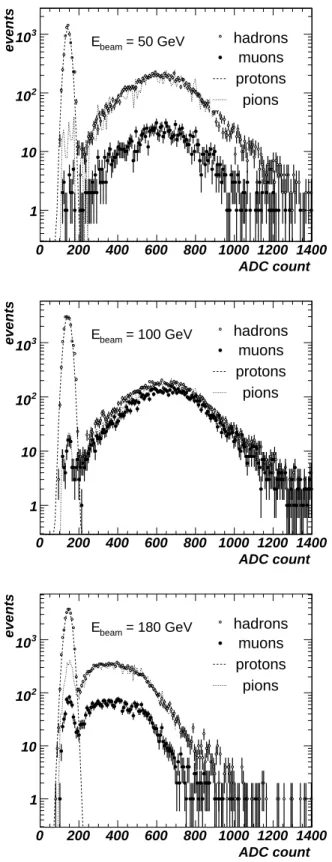
The Cherenkov counter is used to discriminate pions from protons. The distribution of the Cherenkov counter signal (in ADC counts) is shown in Fig.5

for beam energies of 50, 100 and 180 GeV.

The peak in the low signal region is compatible with the pedestal distribution and corresponds to particles leaving no signals in the Cerenkov counter like, e.g. mostly to protons. The shape of the proton distribution can therefore be well modelled with a Gaussian.

The broad distribution in Fig. 5, peaked at larger Cherenkov signals, is mainly due to pions and muons. Its shape can be described by a Poisson distri-bution with a mean value that corresponds to the 2−3 photo-electrons registered by the photo-multiplier (depending on the pressure settings). Since the distribu-tion is also smeared by the finite resoludistribu-tion, it cannot be described analytically. A noticeable fraction of the events does not generate a signal in the Cherenkov counter and therefore exhibits a tail that extends also to the pedestal zone.

To estimate the residual contamination of pions in the sample of protons and the contamination of protons in the sample of pions, muons identified by

ADC count 0 200 400 600 800 1000 1200 1400 events 1 10 2 10 3 10 hadrons muons protons pions = 50 GeV beam E ADC count 0 200 400 600 800 1000 1200 1400 events 1 10 2 10 3 10 hadrons muons protons pions = 100 GeV beam E ADC count 0 200 400 600 800 1000 1200 1400 events 1 10 2 10 3 10 hadrons muons protons pions = 180 GeV beam E

Figure 5: Cherenkov counter response to hadrons and muons at 50, 100 and 180 GeV. Closed circles denote the measurement for hadrons. Open circles correspond to muons. The dashed line is a Gaussian fit to the pedestal distribution. The dotted line corresponds to the shape of pions estimated from the muon measurements.

the calorimeter are used to estimate the shape of the pion distribution in the low signal region (see open circles in Fig.5)13_.

Together with the Gaussian describing the proton peak the muon distribu-tion is scaled to describe the measured hadron Cherenkov signal distribudistribu-tion (see dashed and dotted line in Fig. 5). The adjusted muon Cherenkov signal distributions describes the hadron data within the statistical uncertainties in the region, where no contribution from protons is expected. From this fit the pion (proton) contamination in the proton (pion) sample can be estimated by calculating the number of events below (above) the chosen cuts.

The pion contamination in the sample of protons is summarized in Table1. A sharp increase of the contamination is observed at 180 GeV. This is a con-sequence of non-optimal pressure settings, leading to a visible efficiency loss of pions.

Since at E = 180 GeV the contamination is quite large, all observables measured for protons are corrected using the determined fraction of pions in the proton sample and the measured observables for pions. This is possible, because the proton contamination in the pions sample, as evaluated, is seen to be comparatively small.

The proton contamination in the pion sample is found to be negligible at all energies, if the assumption is made that the efficiency that protons give a signal in the Cerenkov counter is zero. This assumption is well justified for the low energy runs. For the run at E = 180 GeV an upper limit at 95% confidence level on the proton contamination of about 9.0% has been estimated. In the following for all runs all observables are not corrected for proton contamination, but for the E = 180 GeV run a possible contamination of up to 9.0% leads to a systematic uncertainty.

The shape of the Cherenkov counter spectra (see Fig.5) does not leave much room for a third possible hadron species in the beam, kaons in particular. This is also consistent with the estimation of the kaon fraction in the hadron beam estimated by MC simulations to be less than about 5 % [16] at 180 GeV and less at lower energy.

5. Calibration and Corrections 5.1. Electronics and Detector Calibration

Details of the calibration of TileCal for the test-beam data taken in 2002 and 2003 are given in ref [16]. Here, only a short summary is given.

The charge injection system (CIS) calibrates the response of the read-out electronics and a radioactive cesium source (Cs) is used to measure the optical response and to equalize the cell response. The measured channel energy is

13

Due to the small mass difference of muons and pions (as compared to the one between pions and protons), muons are expected to closely reproduce the pion distribution of the Cherenkov response in the full signal range.

reconstructed by:

Erecchan= FADC→pC· FCs· Afit, (2) where Afitis the amplitude (corrected for the pedestal) of the measured samples, the factor FADC→pCis the electronic calibration factor measured with the CIS system [17], FCs corrects for cell non-uniformities using the cesium data. The cell energy is reconstructed as the sum of the two channels each read-out by one PMT.

The signal calibrated with the CIS- and the Cs-system is converted to an absolute energy using a calibration factor (FpC→GeV) that is obtained using electrons. This calibration factor defines the “electromagnetic scale”. The re-sponse of the TileCal cells of about 10% of the TileCal modules installed in the ATLAS detector has been studied using electron test-beams in 2002 and 2003 [18]. The average response of high energetic electrons impinging at a po-lar angle of 20o _{on the TileCal divided by the beam energy is defined as the} FpC→GeV calibration factor14. It is measured to be FpC→GeV = 1.050 ± 0.003 pC/GeV. The cell response variation is 2.4 ± 0.1% [18,16]. The dominant part of the residual cell non-uniformity of about 2% for electrons is due to differences in the optical properties of the tiles and the read-out fibres (intra-cell)15_.

The resulting RMS spread of the pion response is 1.5±0.4% [16]. This spread includes the cell-to-cell and the module-to-module variation. The intrinsic pion response variation in one module is about 0.6 − 0.7%. It is mainly due to tile-to-tile differences estimated to be 0.5% and due to the uncertainty in the CIS calibration that contributes with 0.42%.

Most of the results in ref. [16] are obtained with beams impinging in the projective geometry, relevant for the understanding of the calorimeter response in proton-proton collisions. However, the TileCal in the test-beam configuration analysed here has a different behaviour.

The electron signal is defined as the sum of the first and the second cell that are hit by the impinging beam. The signal-to-energy conversion factor for electrons impinging from the side is determined by the ratio of the electron signal to the beam energy and is found to be 1.075 pC/GeV. This value has been found by averaging the results from electrons in the same runs as used for the pion analysis. The value is consistent with the result from the projective geometry, if the electron response variation with the impact angle as obtained from Monte Carlo simulations [16] is taken into account.

The muon response normalized to the transversed path length per cell has been measured. The cells give the same response within 5 % which is in agree-ment with the results found in ref [16].

14

Due to the varying size of the tiles and the iron absorber as a function of the particle impact point, the electrons response varies by about 10% between small angles η = 0 and large angle η = 0.65[18,16].

15

Such differences can be determined by the Cs-calibration system, but not corrected for, since the smallest read-out entity is a cell and the particle impact on the cell is not known a-priori.

The electron response normalized to the beam energy for electron between 20 to 180 GeV has been found to be linear within 1% using several different data sets. Since the electron beam can only be used to calibrate the edge cells of the TileCal a cell inter-calibration procedure based on the Cs-system that equalizes the BC and D cells with respect to the A cells is needed. This procedure needs to take also geometrical effects into account [18]. Since the electromagnetic scale has been determined using the BC-cell, in this analysis this cell is used as the reference and the response in the A-cells and D-cells is changed by 0.976 and 1.062, respectively.

5.2. Corrections for Detector faults

In the 2002 test beam set-up half of the Barrel Module 0 had no read-out electronics. To overcome this limitation, for each beam energy two runs were taken, with the beam hitting opposite sides of the production Barrel Module. In this manner, the symmetry of the set-up around η = 0 allowed to measure, in separate runs, the average energy depositions in the upstream and downstream halves of Module 0. The mean energy deposition as well as the longitudinal shower profile can then be on average reconstructed from these two measure-ments.

The correction for the mean energy for the non-working part of Module 0 is rather small. It is clear, however, that the RMS can not be corrected with this procedure. The non-working part of the Module 0 leads to an overestimation of the RMS. However, the effect can be estimated by the MC simulation and is found to be negligible. The biggest effect is observed at the highest energy where it reaches 0.1%.

The functioning of the PMTs is checked by selecting muons in the hadron beams impinging at various lateral positions on the calorimeter. Since muons deposit uniformly along their path they are a good tool to check the PMT response (calibration, noise, etc.).

Only a few cases of PMT with unexpected low signals were observed. In this case the PMT energy was set to zero and the energy of the PMT reading out the opposite side of the cell was multiplied by a factor of 2.

[GeV] beam E 20 50 100 180 20 50 100 180

)

/(eE

E

pion

proton

Figure 6: Measured total energy divided by the beam energy for pions (closed circles) and protons (open circles) as a function of the beam energy. The total energy is presented on the electromagnetic energy scale. Shown are statistical uncertainties together with an uncorrelated systematic uncertainty of 0.7% added in quadrature (see section8.1).

6. Data Analysis and Results 6.1. Mean Energy Response

The measured mean total energy, normalized to the beam energy, is referred to as the response of the calorimeter. It is shown for pions and protons in Fig.6. For pions, the response increases by about 7% from 20 to 180 GeV. The increase for protons is steeper.

Fig.7 shows that for all energies the response is larger for pions, and that the ratio of the pion to proton response decreases towards higher energies. Only statistical uncertainties are shown. Most of the systematic uncertainties cancel in the ratio.

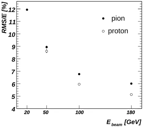
6.2. Energy Resolution

The resolution defined as the root mean square divided by the mean energy (RMS/E) shown in Fig.8is about the same for pions and protons at low energies and is better for protons at higher energies (E ≥ 100 GeV).

Since the calorimeter is very long the hadronic shower is fully contained and there is no low energy tail from longitudinal leakage. Therefore it is enough to quote the RMS of the energy distribution, since it give the same result as a Gaussian fit around the peak value.

[GeV] beam E 50 100 180 50 100 180 tot p

/E

E

Figure 7: The ratio of the mean energy measured for pions and protons as a function of the beam energy. Only statistical uncertainties are shown.

These results (mean and RMS) are not biased by the cut on the average energy density. They stay stable within 0.2% when the cut on the energy density is removed in the MC simulation. The results of both means and resolutions are corrected for the measured beam contamination.

6.3. Shape of the Energy Distribution

All the previous measurements reflect qualitatively the non-compensating nature of the TileCal that leads to a different response to the hadronic and electromagnetic energy depositions during the shower development. They are, moreover, consistent with a larger electromagnetic energy fraction in pion in-duced showers.

The different response of the TileCal to the electromagnetic and hadronic shower components is also clearly illustrated in Fig. 9, where the energy dis-tribution normalized to the mean energy hEtoti is compared for pions and pro-tons at 100 GeV. The shapes are fitted by a Gaussian in the region between 0.8 < Etot/hEtoti < 1 and extrapolated to the region 1 < Etot/hEtoti < 1.2, where the energy response is larger than the mean and more events are seen than would be expected, if the whole energy distribution was Gaussian. In this region the electromagnetic energy fractions appears to be higher.

The bias introduced by the particle identification cuts are smaller than 2 % up to values around 1.1 and then increases up to 10 % towards the end of the ratio.

[GeV]

E

20

50

100

180

20

50

100

180

RMS/E [%]

4

5

6

7

8

9

10

11

12

pion

proton

Figure 8: Energy resolution (RMS/hEi) for pions (closed circles) and protons (open circles) as a function of the beam energy. Overlaid as a curve is a fit to the pion energy resolution. Only statistical uncertainties are included. The hadronic shower is fully contained in the calorimeter. The calorimeter length is more than 20λ.

> tot /<E tot E 0.6 0.7 0.8 0.9 1 1.1 1.2 1.3

Norm. Events

pion

proton

Figure 9: Measured total energy distribution divided by the mean total energy for pions (closed circles) and protons (open circles). Only statistical uncertainties are included.

>

/<E

E

0.7

0.8

0.9

1

1.1

1.2

1.3

1.4

1.5

Data/Gaussian

1

10

pion

proton

Figure 10: Bin to bin ratio of the reconstructed energy distribution and its Gaussian fit for protons (open circles) and pions (closed circles) as a function of relative reconstructed energy Etot/hEtoti. The fit was carried out in the region below 1 and extrapolated to the region

The clear asymmetry between low and high energy depositions is even more visible in the ratio of the data to the extrapolated Gaussian fit16 _{shown in}

Fig.10. In the region Etot/hEtoti < 1, where the energy is lower than the mean, the measured shape is compatible with a Gaussian. In the region above the mean, for both pions and protons, an increasingly larger number of events is seen in the measured distribution. This effect is more pronounced for pions than for protons. This nicely illustrates the different pion and proton responses in the calorimeter: protons have a more symmetrical shape with a less pronounced left-right asymmetry than pions, as a consequence of the larger size and of larger fluctuations in the electromagnetic content of pion induced showers.

6.4. Longitudinal Shower Profiles

The measured longitudinal shower profiles for pions and protons are pre-sented in Fig.11. They represent the mean energy as a function of the depth of the layer. The depth is taken to be the size of the B sub-cell, since most of the energy is deposited here. The normalization is done with respect to the mean total measured energy17_.

The measurements extend up to 20 λ in depth. On average, both types of hadron showers quickly deposit their energy and reach the point within the first few λ in depth where the mean energy deposition is maximal. The average energy deposition then exponentially decreases towards the end of the shower and is down by approximately four orders of magnitudes at 15 λ.

The long tail at the end of the shower becomes flatter, when the mean energy loss per cell is compatible to the noise fluctuations. The measurement is stopped at this depth.

The ratio of the profiles of showers induced by pions and protons is presented in Fig.12. Since the statistical uncertainties of the measured longitudinal pro-files are relatively higher at the end of showers, the ratios are only presented for a limited range of depth that depends on the energy. At 50 GeV the pion to proton ratio is flat and close to 1, up to a depth of 10 λ. It decreases with depth at higher energies.

This behavior may be explained by the higher proton interaction cross-section with iron nuclei. Therefore, pions, on average, penetrate deeper in the calorimeter. This results in fewer hadronic interactions initiated by pions in the first one or two cells, which, however, are characterized by a higher fraction of neutral pions. These two differences in the underlying mechanism of the shower development for pions and protons have opposite effects on the longitudinal pro-files. This might explain the similar longitudinal shower development for pion and protons at 50 GeV.

The bias resulting from the electron rejection cut (see Section4.1) on the pion and proton longitudinal shower profile can be evaluated by using the results of

16

To obtain the ratio, the integral of the fitted Gaussian is calculated for each bin, divided by the bin width and by the number of data events in this bin.

17

In this section the longitudinal profile are not corrected for the effect of the projective form of the BC cells. Such corrections will be discussed and applied in Section8.3.

]

λ

z [

5

10

15

20

25

]

λ

dE/dz [GeV/

10

10

10

1

10

10

]

λ

z [

5

10

15

20

25

]

λ

dE/dz [GeV/

10

10

10

1

10

10

Figure 11: Pion and proton longitudinal shower profile at various energies. Only statistical uncertainties are shown.

]

λ

z [

5

10

15

20

25

/(dE/dz)

(dE/dz)

0

0.2

0.4

0.6

0.8

1

1.2

1.4

Figure 12: Ratio of the longitudinal profiles for protons and pions at various energies. Only statistical uncertainties are shown.

simulations with different hadronic interaction models where electron and pions or protons are mixed together according to the measured beam composition and by comparing the results with and without the electron rejection cuts. A systematic uncertainty of maximally 4% is found on the measured value in the first layer using the QGSP physics list. As will be shown later, QGSP predicts too short and too narrow hadronic showers and the systematic uncertainty is therefore overestimated. Using the LHEP BERT physics list a bias of only 1% was found on the same quantity.

Since the normalization of the longitudinal profile is chosen to be the total energy, also other layers can be affected. However, the bias due to the electron rejection cut is at least 2 times smaller. The systematic uncertainty introduced by the muon identification cut can be evaluated by looking at the observables with and without the cut on the discriminant (see Section4.1) as well as using the results of simulation. The resulting systematic uncertainty is found to be smaller than the statistical uncertainty.

The systematic uncertainty due to a possible proton contamination in the pion sample for a beam energy of 180 GeV has been evaluated by moving the Cerenkov signal cut further to higher values (see Section 4.5). This control sample only contains very pure pions. The ratio of the longitudinal energy profiles in the standard and the control samples is the same up to about 10λ. From this point onwards it slowly increases and reaches about 10% at 15λ. This ratio is considered a systematic uncertainty in the measurement.

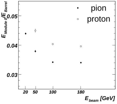
6.5. Lateral Spread

In Fig. 13the ratio of the energy deposit in the Module 0 and in the pro-duction Barrel Module is presented. The distance of the beam impact point in the Barrel Module to the Module 0 is 0.6 λ. The ratio is a simple estimator of the lateral spread of the shower. Since the measured ratio is larger for pions than for protons, pion induced showers are laterally narrower. This may come as surprise, since pion showers have just been shown to be longer.

This observation might also be qualitatively explained by the difference in the electromagnetic energy contents of pion and proton showers. Most of the energy is produced near the core of the shower. Since electromagnetic showers are compact, the electromagnetic energy is deposited relatively close to the core of the shower. Assuming that the hadronic energy deposited in the pion and the proton showers has the same lateral spread, the above defined ratio will be as much different as the inverse ratio of the electromagnetic energy fraction. Since the electromagnetic energy fraction is larger by about 20 % (see Section4.5), the 20% larger lateral spread for protons is consistent with this interpretation.

[GeV]

E

20

50

100

180

20

50

100

180

/E

E

0.03

0.04

0.05

pion

proton

Figure 13: Ratio of the energy deposition in the Module 0 and in the Barrel Module charac-tering the lateral spread of pion and proton showers as a function of the beam energy. Besides the statistical uncertainties also a systematic uncertainty of 1% is included.

7. Comparisons to Monte Carlo Simulations

In this section the response, the resolution, the mean longitudinal shower profile as well as the lateral spread are compared to Monte Carlo simulations. 7.1. Response

Fig.14shows the comparison of the data with the Monte Carlo simulation for the pion and proton response. The comparison is performed at the electro-magnetic scale. For the MC the electroelectro-magnetic energy scale is obtained using the results from the electron simulations. The normalization is chosen such that the mean electron energy in MC equals to the beam energy.

The LHEP physics list predicts a response that is about 10% lower than the data. The QGSP physics list is closer to the data, but also 5% lower. Adding the Bertini cascade increases the response by about 5 − 10% and improves the description of the energy dependence of the response. However, the response in the QGSP BERT physics list is about 3% higher than the one in the data. For the LHEP BERT physics list the response is 1% lower.

7.2. Resolution

The comparison of the resolution in the Monte Carlo simulation to the one in the data is shown in Fig.15.

For both MC simulation models LHEP and QGSP, the RMS spread is larger by about 10 % in the Monte Carlo simulation than found in the data. Adding the Bertini cascade decreases the simulated resolution by about 15%. For pions this results in a resolution that is 5% narrower than the one in the data. For protons the simulation describes the data well except for a proton energy of 50 GeV.

Taking into account the good description of the mean total energy and the RMS spread by the Bertini models, in particular, by QGSP BERT, we conclude that adding the Bertini cascade model leads to a better description of TileCal energy resolution.

7.3. Longitudinal Shower Profile

The measured pion shower profiles are compared to all physics lists for all energies in Fig. 16. To make the direct comparison easier, the ratio of the simulated shower profiles to the ones measured in the data are shown. The predictions of the hadronic physics lists vary significantly.

The LHEP physics list describes the pion data above 50 GeV quite well, i.e. within 10% for the first 10 λ. At low energies the simulated showers are, however, too short. For instance, for pions with an energy of 20 GeV the mean deposited energy is 40% lower at a shower depth of 10λ18_.

18

Note, that for 20 GeV energy almost the same model (LEP) is used for both physics lists, QGSP and LHEP.

[GeV]

E

MC/Data

0.85

0.9

0.95

1

1.05

1.1

[GeV]

E

MC/Data

0.85

0.9

0.95

1

1.05

1.1

Figure 14: Ratio of the mean energy in the Monte Carlo simulation to the one in the data as a function of the beam energy for four physics list for pions (a) and protons (b). Both data and MC are normalized to the electromagnetic scale. Only statistical uncertainties are included, they are smaller than the marker size. The overall normalisation uncertainty is 1%.

[GeV]

E

MC/Data

0.8

0.9

1

1.1

1.2

1.3

1.4

1.5

[GeV]

E

MC/Data

0.8

0.9

1

1.1

1.2

1.3

1.4

1.5

Figure 15: Ratio of the RMS of total energy distribution in the Monte Carlo simulation to one in the data as a function of the beam energy for four physics list for pions (a) and protons (b). Only statistical uncertainties are included.

] λ z [ 5 10 15 20 25 MC/Data 0 0.2 0.4 0.6 0.8 1 1.2 1.4 1.6 1.8 pion 20 GeV 50 GeV 100 GeV 180 GeV LHEP ] λ x [ 5 10 15 20 25 MC/Data 0 0.2 0.4 0.6 0.8 1 1.2 1.4 1.6 1.8 pion 20 GeV 50 GeV 100 GeV 180 GeV QGSP ] λ z [ 5 10 15 20 25 MC/Data 0 0.2 0.4 0.6 0.8 1 1.2 1.4 1.6 1.8 pion 20 GeV 50 GeV 100 GeV 180 GeV LHEP_BERT ] λ z [ 5 10 15 20 25 MC/Data 0 0.2 0.4 0.6 0.8 1 1.2 1.4 1.6 1.8 pion 20 GeV 50 GeV 100 GeV 180 GeV QGSP_BERT a) b) c) d)

Figure 16: Ratio of various MC simulations to data for the pion longitudinal shower profile description at various energies. Only statistical uncertainties are shown.

The QGSP physics list predicts too short pion showers over the full energy range. The mean deposited energy is too large at the beginning (+20%) and too low at the end of the shower (−40% at 10λ).

Adding the Bertini inter-nuclear cascade model makes showers longer in both physics lists, LHEP and QGSP. This is probably due to the larger number of low energy neutrons produced by this model. For the LHEP physics list above 50 GeV the showers are too long, while at 20 and at 50 GeV the data are described within about 10%.

In the case of the QGSP physics list, adding the Bertini cascade leads to noticeable improvements in the description of the data. In the first 10 λ the data are reproduced within a precision of ±20%. At 10 λ LHEP BERT is 20 % too high, while QGSP BERT is 20 % too low. Unlike LHEP, in case of the QGSP list (with or without Bertini’s model) the underestimation of the longitudinal shower profiles is consistent in the energy range 20 to 180 GeV. 7.4. Lateral Spread

Fig.17shows the ratio of the longitudinal shower profile of data and Monte Carlo simulations for protons. The LHEP physics list describes the data quite well above 50 GeV, but fails at 20 GeV. The QGSP physics list predicts too short showers in the full energy range. Using the Bertini model in addition makes shower longer and a better agreement to the data is observed, but the proton shower is still shorter. The description of the 50 GeV shower profile is worse than the one at 100 and 180 GeV. The shower starts and ends to early. At the beginning of the shower the mean energy deposited is +20% and at a shower depth of 10λ 50% less energy is deposited.

The description of the data for protons is in general worse than the one for the pions for all physics lists.

The ratio of energy deposition in the Barrel and Module 0 for data and simulation is presented in Fig.18. Both physics lists, QGSP and LHEP, predict showers with a lateral spread significantly narrower than the one measured in the data for both pions and protons. The description of QGSP is worse than the one of LHEP. Adding the Bertini cascade leads to a better description of the data for both physics lists. However, the simulated showers are still narrower. LHEP BERT gives the best description, but the shower are predicted to be a bit wider than the ones in the data.

7.5. Summary

In conclusion, QGSP predicts showers that are too short and too narrow. LHEP reproduces the longitudinal shower shape correctly for E > 50 GeV, but the showers are too narrow. Adding the Bertini cascade model makes showers longer and wider. For QGSP this reproduces the data better, while for LHEP the showers become too long.

The physics lists QGSP and LHEP, together with the Bertini cascade model were therefore used to evaluate the electron contamination in the pion sample and to estimate the systematic uncertainty introduced by the cut on the average energy density (see Section4.1).

] λ z [ 5 10 15 20 25 MC/Data 0 0.2 0.4 0.6 0.8 1 1.2 1.4 1.6 1.8 proton 50 GeV 100 GeV 180 GeV LHEP ] λ z [ 5 10 15 20 25 MC/Data 0 0.2 0.4 0.6 0.8 1 1.2 1.4 1.6 1.8 proton 50 GeV 100 GeV 180 GeV QGSP ] λ z [ 5 10 15 20 25 MC/Data 0 0.2 0.4 0.6 0.8 1 1.2 1.4 1.6 1.8 proton 50 GeV 100 GeV 180 GeV LHEP_BERT ] λ z [ 5 10 15 20 25 MC/Data 0 0.2 0.4 0.6 0.8 1 1.2 1.4 1.6 1.8 proton 50 GeV 100 GeV 180 GeV QGSP_BERT a) b) c) d)

Figure 17: Ratio of various MC simulations to data for the proton longitudinal shower profiles at various energies. Only statistical uncertainties are shown.